EPR Pairs from Indefinite Causal Order

Abstract

We develop a novel protocol to achieve entanglement creation between qubit pairs by making a qubit pair experience an indefinite causal order process. In particular, our protocol does not need two qubits to interact with each other, meaning that only local operations are applied on individual qubits. In order to demonstrate the usage of the protocol, we first identify the conditions under which, EPR pairs, the maximally entangled states emerge from our protocol. Furthermore, we show that, although our protocol is not deterministic, the success probability of getting an EPR pair could be non-vanishing, even comparably high enough. Our result not only sheds new light on entanglement creation, but revealing that a quantum switch has further potential to be explored.

Introduction.— In quantum physics, especially in the field of quantum information science, entanglementHorodecki et al. (2009); Brunner et al. (2014), a form of quantum correlation is recognized as an essential resource which serves to play indispensable rolesXu et al. (2020) to gain advantage over their classical counterparts in wide-ranging tasks including quantum teleportationBose et al. (1999); Bennett et al. (1993); Nielsen and Chuang (2011), quantum metrologyGiovannetti et al. (2006) and quantum cryptographyJennewein et al. (2000); Ekert (1991), to mention a few. Seeking for appropriate ways of creating this non-classical correlation therefore becomes crucial and is of considerable interest.

Interactions between quantum systems can give arise to entanglementAbanin et al. (2019), specifically in quantum many-body systems where strong interaction takes place a huge amount of entanglement may be created out of the complicated dynamics. Exploiting interactions has given birth to numerous methods for generating entanglement in different contextsPan et al. (2012), through direct interactions, or by making use of some mediator systemsBraun (2002). Nevertheless, it still remains to be explored whether we can achieve the goal in different ways especially when a direct interaction between two quantum system parties is absent.

In this Letter, we propose a novel method which allows one to accomplish the task of creating entangled states between a pair of two-state quantum systems, or qubits. Our approach does not require the two qubits to interact with each other or even with a third party. The resulting entangled states can reach the peak, the maximally entangled states under certain conditions which we will identify in this work. Moreover, due to the fact that our protocol is probabilistic, to characterize our proposal, we also provide analysis of the success probability to obtain a maximally entangled state. This novel result is closely related to a class of counter-intuitive quantum processes whose causal order exhibits non-separabilityOreshkov et al. (2012); Goswami et al. (2018); Rubino et al. (2017); Procopio et al. (2015).

Quantum switch realizing novel quantum processes.— We start by introducing the quantum switchChiribella et al. (2013); Rubino et al. (2021); Guérin et al. (2016); Araújo et al. (2014), and before that we review some prerequisites which is necessary to understand this novel physical resource. Recall that the evolution of a quantum system is dictated by the Schrödinger equation, taking in account specific measurement processes, one could in principle find how the system evolves toward future. Equivalently, an evolved state can be obtained by treating it as the output of the system passing a quantum channel, which is usually described by a completely positive and trace preserving (CPTP) map. In addition, it is of convenience to use the operator-sum representation for describing the action of a quantum process, in which case a set of operators called Kraus operators enables one to obtain the transformed state of a quantum system. Suppose that we have a channel $\mathcal{M}$ which is associated with a set of Kraus operators $\{K_{i}\}$. With the initial state $\rho$ (the time argument has been suppressed) of a system, the evolved state will then be $\widetilde{\rho}=\sum_{i}K_{i}\rho K_{i}^{\dagger}$, where the operators satisfy $\sum_{i}K_{i}^{\dagger}K_{i}=\mathbb{I}$, and an evolved state is marked with a tilde for the purpose of distinguishing from the initial state.

In cases where one encounters multiple processes, a fixed background causal structure is assumed even in the conventional setting of quantum mechanics. For instance, say we have two processes taking place in the space-time, one of the processes must exist in the causal past (or future) of the other. However, this assumption may not necessarily be true — modifications should be made on the conventional notion of causality if one takes into consideration the properties of both quantum mechanics and general relativity. In simple words, nondeterminism of the quantum theory and the dynamical causal structure in general relativity may give rise to novel causal structures. What this implies is that one may expect the existence of processes whose causal order becomes indefinite in a theory of quantum gravity, the main goal of which is to reconcile the two above-mentioned solid pillars of modern physics.

There are processes where the causal order among events cannot be described by classical physics. In particular they are referred to as indefinite causal order processes. Let us call two arbitrary processes $\mathcal{M}$ and $\mathcal{N}$ respectively. Especially in our consideration, $\mathcal{M}$ and $\mathcal{N}$ are modeled as two quantum channels. Depending on the way they locate in the space-time, $\mathcal{M}$ can exist in the causal past of $\mathcal{N}$, which we denote by $\mathcal{M}\circ\mathcal{N}$. Similarly, the composition of two channels in the reverse order $\mathcal{N}\circ\mathcal{M}$ means that $\mathcal{N}$ locates in the causal past of $\mathcal{M}$. In conventional scenarios, no other possibilities for their causal order are conceivable, however, indefinite causal order relaxes the constraint that any pair of events has to obey a fixed causal order. One can understand an indefinite causal order process by imaging that — $\mathcal{M}\circ\mathcal{N}$, which corresponds to the process where $\mathcal{N}$ happens in the future of $\mathcal{M}$ is being in superposition with $\mathcal{N}\circ\mathcal{M}$. It is doubtful that if our physical word really allows for indefinite causal order happening rather than remaining just as an unrealistic model. In fact, regardless of appearing counter-intuitive, an indefinite causal order can be realized through a novel physical resource known as quantum switch.

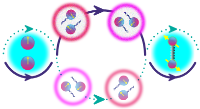
Figure 1: The qubit $\mathcal{Q}^{A}$ and qubit $\mathcal{Q}^{B}$ start from the left side initialized in a separable state, following two processes applied on them, where we ruled out interaction between the qubit pair. Two processes are represented by a red (blue) circle, which corresponds to $\mathcal{M}$ and $\mathcal{N}$, respectively. Here the solid and dotted curves are used to denote the superposition of temporal order of events. In our proposal, under proper conditions an EPR pair may appear at the end of the process.

A quantum switch is an example which exhibits indefinite causal order, where an auxiliary system, i.e., a control qubit serves to control the order of events. In addition to the control qubit, another one is used as the target qubit to perform specific tasks. In order to illustrate how a quantum switch works, we examine its mathematical description in the Kraus decomposition representation,

$$V_{ij}(t)= \outerproduct{1}{1}^{C}\otimes{K^{m}_{i}}(t/2){K^{n}_{j}}(t/2)$$

$$+ \outerproduct{0}{0}^{C}\otimes{K^{n}_{j}}(t/2){K^{m}_{i}}(t/2).$$ (1)

Here the symbol $\otimes$ separates the operators which act on the controls and on the target, $\{K_{i}^{m}\}$ stands for the Kraus operator set for $\mathcal{M}$, and the same for $\{K_{i}^{n}\}$. Taking the viewpoint that a quantum switch is a resource transforming input channels to new ones may help capture its function. To interpret the action performed on the target qubit, we consider the initial state of the control qubit, which is denoted by $\rho_{C}=\outerproduct{\psi}{\psi}^{C}$. If the control qubit is initialized in the state $\outerproduct{\psi}{\psi}^{C}=\outerproduct{0}{0}^{C}$, the resulting action will be $\mathcal{M}\circ\mathcal{N}$, whereas it gives the reserve, that is $\mathcal{M}\circ\mathcal{N}$ when $\outerproduct{\psi}{\psi}^{C}=\outerproduct{1}{1}^{C}$.

EPR pairs emerge from local operations.— The system we shall use to illustrate our result consists of a pair of qubits, let us call them qubit $\mathcal{Q}^{A}$ and qubit $\mathcal{Q}^{B}$, whose Hamiltonian operators are

$$\hat{\mathcal{H}}^{A(B)}=\omega_{z}^{A(B)}\sigma_{z},$$ (2)

where a constant $\omega_{z}^{A}$ whose value is taken to be the same as $\omega_{z}^{B}$ and $\sigma_{z}$ is the Pauli-$z$ operator. Since $\omega_{z}^{A}$ equals $\omega_{z}^{B}$, let us drop the superscript so that $\omega_{z}\coloneqq\omega_{z}^{A}=\omega_{z}^{B}$. The Pauli-$z$ is defined as $\sigma_{z}=\outerproduct{0}{0}-\outerproduct{1}{1}$, where $\{\ket{0},\ket{1}\}$, the eigenstates of $\sigma_{z}$ constitute an orthonormal basis for a two-dimensional Hilbert space. We want to deal with both of $\mathcal{Q}^{A}$ and $\mathcal{Q}^{B}$ at the same time, which is made by first obtaining the operators acts on the product of the two individual Hilbert spaces. The joint Hamiltonian is simply the sum of the individual ones, which reads $\hat{\mathcal{H}}^{AB}=\hat{\mathcal{H}}^{A}\otimes\mathbb{I}^{B}+\mathbb{I}^{A}\otimes\hat{\mathcal{H}}^{B}$. Here, we have chosen to write down the tensor product structure explicitly to highlight on which Hilbert space an operator acts. We then define the density operators in terms of the eigenstates of qubit Hamiltonian as $\rho_{A(B)}=p_{0}^{A(B)}\outerproduct{0}{0}^{A(B)}+p_{1}^{A(B)}\outerproduct{1}{1}^{A(B)}$ to represent the states of qubit $\mathcal{Q}^{A}$ and qubit $\mathcal{Q}^{B}$. Just as what is for the Hamiltonian operators, the joint density operator can be written as $\rho_{AB}=\rho_{A}\otimes\rho_{B}$.

In what follows let us first make an assumption that only local operations are allowed for both of the two qubits, which equivalently says that no interaction take place between our qubits $\mathcal{Q}^{A}$ and $\mathcal{Q}^{B}$. Before preceding, recall that we are going to exploit the novel resource quantum switch to generate entanglement, which generally requires more than one process. In this regard, we introduce auxiliary Hamiltonian operators which collectively with the qubit Hamiltonian constitute the generator of the time propagator. Especially, we will relate the auxiliary Hamiltonians with a set of coefficients. This is done by expressing an auxiliary Hamiltonian as a linear combination of Hermitian operators other than the Pauli-$z$ operator. Let us assign the name $\mathcal{M}$ and $\mathcal{N}$ to the two processes. To illustrate our idea we have sketched the novel scenario in Fig. 1.

We now construct the auxiliary Hamiltonian first for the process $\mathcal{M}$, let us denote by $\hat{\mathcal{A}}_{M}=\chi_{M}^{A}\sigma_{x}\otimes\mathbb{I}^{B}$ which acts on the qubit $\mathcal{Q}^{A}$. For the process $\mathcal{N}$, the Hamiltonian $\hat{\mathcal{A}}_{N}=\mathbb{I}^{A}\otimes\chi_{N}^{B}\sigma_{x}$ acting on $\mathcal{Q}^{B}$ plays the similar role as $\hat{\mathcal{A}}_{M}$ does. Here the $\chi_{M(N)}^{A(B)}$ are constants and the Pauli-$x$ operator $\sigma_{x}$ is defined in terms of eigenstates of $\sigma_{z}$ as $\sigma_{x}=\outerproduct{0}{1}+\outerproduct{1}{0}$. Besides the local operation assumption, we further rule out the possibility of the qubits being in contact with any other systems, thus it leads us to write down the Kraus operator for $\mathcal{M}$ as $K^{m}(t)={\exp}[-i\cdot(\hat{\mathcal{H}}^{AB}+\hat{\mathcal{A}}_{M})\cdot t]$, and $K^{n}(t)={\exp}[-i\cdot(\hat{\mathcal{H}}^{AB}+\hat{\mathcal{A}}_{N})\cdot t]$. Note that we have made $\hbar=1$ here.

Table 1: Conditions for an indefinite causal order process to generate maximally entangled states. For a qubit pair, there are more than one way to get maximally entangled, thus we label the four possibilities with $\mathbb{A}$, $\mathbb{B}$, $\mathbb{C}$ and $\mathbb{D}$ respectively. In this table, we use a state vector instead of a density operator to represent a quantum state. All the states in the last column are reduced states corresponding to the $\ket{-}$ measurement results associated with the control qubit.

	$\ket{\psi}_{AB}$	$\hat{\mathcal{A}}_{M}(\hat{\mathcal{A}}_{N})$	$\widetilde{\ket{{\psi}}}_{AB}^{-}$
$\mathbb{A}$	$\ket{00}$	$\chi_{M}^{A}/\chi_{N}^{B}=1$	$(\ket{01}-\ket{10})/\sqrt{2}$
$\mathbb{B}$	$\ket{00}$	$\chi_{M}^{A}/\chi_{N}^{B}=-1$	$(\ket{01}+\ket{10})/\sqrt{2}$
$\mathbb{C}$	$\ket{01}$	$\chi_{M}^{A}/\chi_{M}^{B}=-1$	$(\ket{00}-e^{i\phi}\ket{11})/\sqrt{2}$
$\mathbb{D}$	$\ket{01}$	$\chi_{M}^{A}/\chi_{M}^{B}=1$	$(\ket{00}+e^{i\phi}\ket{11})/\sqrt{2}$

The control system plus the two qubits jointly evolve under the action of the quantum switch, given the initial state $\rho_{CAB}\coloneqq\rho_{C}\otimes\rho_{AB}$, the system will be mapped to become $\widetilde{\rho}_{CAB}=V\rho_{CAB}V^{\dagger}$. We now specify how $\rho_{C}$ and $\rho_{AB}$ are initialized — the control system $\rho_{C}$ begins in a balanced superposition state $\rho_{C}=\sum_{ij}(1/2)\outerproduct{i}{j}^{C}$. For the qubit pair, we assume that they are prepared in a separable state $\rho_{AB}=\outerproduct{0}{0}^{A}\otimes\outerproduct{0}{0}^{B}$.

Aside from specifying the dynamics generator and the initial state, we need to further choose the measurement basis for the quantum switch because a measurement should be taken on the control qubit. In this work, we make the choice of using $\ket{\pm}^{C}\coloneqq(\ket{0}^{C}\pm\ket{1}^{C})/\sqrt{2}$ for the measurement. The reduced state of $\mathcal{Q}^{A}$ and $\mathcal{Q}^{B}$ is of our interest since it grants us access to the information of the system. Tracing out the control system degrees of freedom after performing the projective measurement yields the result, which can be formally expressed in the following way

$$\widetilde{\rho}_{AB}^{\pm} ={\rm{Tr}}_{C}\big{[}\outerproduct{\pm}{\pm}^{C}\widetilde{\rho}_{CAB}\outerproduct{\pm}{\pm}^{C}\big{]}$$

$$=\sum_{i}\bra{i}^{C}\outerproduct{\pm}{\pm}^{C}\widetilde{\rho}_{CAB}\outerproduct{\pm}{\pm}^{C}\ket{i}^{C},$$ (3)

where we denote two branches of outcome as $\widetilde{\rho}_{AB}^{\pm}$, which up to normalization is a density operator, coming with the probability of ${\rm{Tr}[\widetilde{\rho}_{AB}^{\pm}]}$.

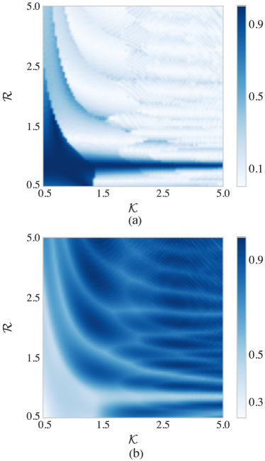
Figure 2: Concurrence of the qubit $\mathcal{Q}^{A}$ and qubit $\mathcal{Q}^{B}$ is shown in $(a)$, and the probability to get such a state is demonstrated in the below $(b)$. The result is obtained by exploring the $[0.5,5.0]\times[0.5,5.0]$ parameter space ($\mathcal{R}$ and $\mathcal{K}$), while keeping $\omega_{z}=1/2$. One notices that high probability outcomes are associated with low concurrence states.

In the following, we investigate the conditions under which a maximally entangled state can be achieved. Furthermore, owing to the probabilistic nature of the control qubit measurement, we mention that the corresponding probability must be taken care. It turns out that in the future where a $\widetilde{\rho}_{AB}^{-}$ appears, we will always obtain a maximally entangled state regardless of the time at which a measurement is performed, as long as the following condition holds. That is $\mathcal{R}^{2}=1$, where $\mathcal{R}$ is the ratio between $\chi_{M}^{A}$ and $\chi_{N}^{B}$, thus $\mathcal{R}=\chi_{M}^{A}/\chi_{N}^{B}$. In cases where the above-mentioned condition is satisfied, the joint system behaves in the following way,

$$\bra{ij}^{AB}\widetilde{\rho}_{AB}^{-}\ket{kl}^{AB}=\begin{cases}\mathcal{G}/2&\text{$(i,k=s$ and $j,l=1-s)$}\\ -\mathcal{R}\mathcal{G}/2&\text{$(i,l=s$ and $j,k=1-s)$}\\ 0&\text{otherwise}.\end{cases}$$ (4)

Here $s=0$ or $1$, with $\mathcal{G}$ being a function of three parameters $\chi_{M}^{A}$, $\omega_{z}$, $t$, and its explicit expression is

$$\mathcal{G} ={\chi_{M}^{A}}^{2}\sin^{2}({\omega_{z}\cdot t})\sin({\Theta\cdot t})$$

$$\times\frac{(2\omega_{z}^{2}+{\chi_{M}^{A}}^{2}/2)\sin({\Theta\cdot t})+({\chi_{M}^{A}}^{2}/2)\sin{(3\cdot\Theta\cdot t)}}{\Theta^{4}},$$ (5)

where $\Theta=\sqrt{\omega_{z}^{2}+{\chi_{M}^{A}}^{2}}/2$. One then easily sees that ${\rm{Tr}[\widetilde{\rho}_{AB}^{-}]}={\mathcal{G}(\chi_{M}^{A},\omega_{z},t)}$. Furthermore, examining $\mathcal{G}$ in details suggests that the maximum value can be reached to be $1/2$ within the region $\omega_{z}\leq\chi_{M}^{A}$, hence we have $0\leq\mathcal{G}\leq 1/2$. In fact, the reduced state in this case, take $\mathcal{R}=-1$ for example, is $(\ket{01}^{AB}+\ket{10}^{AB})/\sqrt{2}$. For another three maximally entangled state, we have summarized in Table 1 the conditions that will yield desirable results, including the initial states of the qubit pair and the forms of auxiliary Hamiltonians. For cases where $\mathcal{R}$ deviates from $\pm 1$, although a reduced state becomes time-independent, a state with some amount of entanglement is still excepted. To show this, recall that concurrence is a measure of the entanglement, and for any qubit pair state, the definition is given by

$$\mathcal{C}(\rho)=\max\big{[}{(\sqrt{\lambda_{1}}-\sqrt{\lambda_{2}}-\sqrt{\lambda_{3}}-\sqrt{\lambda_{4}}),0\big{]}},$$ (6)

where $\lambda_{1},\lambda_{2},\lambda_{3},\lambda_{4}$ are the eigenvalues of the operator $\rho^{\star}=\rho(\sigma_{y}\otimes\sigma_{y})\rho(\sigma_{y}\otimes\sigma_{y})$. We further study the behavior of a entangled qubit pair through evaluating the concurrence. The result is plotted in Fig. 2, where we fix $\omega_{z}$ to be $1/2$ while tuning $\mathcal{R}$ and $\mathcal{K}\coloneqq\chi_{N}^{B}/\omega_{z}$ to observe how the concurrence is affected. To obtain the result we first solve for the point at which the probability to get a $\ket{-}$ measurement result is maximized, the concurrence is then evaluated at the same point. From Fig. 2, one soon recognizes that the concurrence behaves as if it competes with the probability, i.e., in regions where concurrence reaches a relatively high value coincides with low probability realms. Nevertheless, a stripe passing through the area where $\mathcal{R}=1$ is interesting, which is obviously consistent with our analytical results.

Conclusions.— In this Letter, we have proposed a novel method that generates quantum entanglement. By superposing the causal order of two processes, we found that under proper conditions, one has chance of witnessing the generation of entangled states. What’s more, by further restricting on a subset of the conditions, we can even create EPR pairs, the maximally entangled states. What is of our great interest is that unlike other methods that have been proposed so far, in our protocol no interaction between the qubits takes place, thus making it be an interaction-free protocol. To construct our protocol, we identified the conditions that is sufficient for obtaining an EPR pair, and also analyzed the success probability.

Our protocol is in general of probabilistic nature due to the projective measurements made on the control qubit of a quantum switch. A vanishing probability is not desirable no matter what the outcome is. In this regard, we argued that our scheme can actually achieve at least with a probability of $1/2$ for the case of getting the optimal result. While for other cases where the outcome may not necessarily be an EPR pair, we studied in terms of concurrence how the amount of entanglement of an entangled state relates with the corresponding success probability. It then turned out that in general a high concurrence state comes with relatively low probability.

As a novel resource, the quantum switch has shown its advantage in many quantum information tasks, here, we have further expanded horizons by demonstrating its role in this new context.

Note added.— Recently, we learned of a work by Koudia and co-authors who have also investigated the usage of quantum switch to generate entangled quantum statesKoudia et al. .

References

- Horodecki et al. (2009) R. Horodecki, P. Horodecki, M. Horodecki, and K. Horodecki, Rev. Mod. Phys. 81, 865 (2009).
- Brunner et al. (2014) N. Brunner, D. Cavalcanti, S. Pironio, V. Scarani, and S. Wehner, Rev. Mod. Phys. 86, 419 (2014).
- Xu et al. (2020) F. Xu, X. Ma, Q. Zhang, H.-K. Lo, and J.-W. Pan, Rev. Mod. Phys. 92, 025002 (2020).
- Bose et al. (1999) S. Bose, P. L. Knight, M. B. Plenio, and V. Vedral, Phys. Rev. Lett. 83, 5158 (1999).
- Bennett et al. (1993) C. H. Bennett, G. Brassard, C. Crépeau, R. Jozsa, A. Peres, and W. K. Wootters, Phys. Rev. Lett. 70, 1895 (1993).
- Nielsen and Chuang (2011) M. A. Nielsen and I. L. Chuang, Quantum Computation and Quantum Information: 10th Anniversary Edition, 10th ed. (Cambridge University Press, USA, 2011).
- Giovannetti et al. (2006) V. Giovannetti, S. Lloyd, and L. Maccone, Phys. Rev. Lett. 96, 010401 (2006).
- Jennewein et al. (2000) T. Jennewein, C. Simon, G. Weihs, H. Weinfurter, and A. Zeilinger, Phys. Rev. Lett. 84, 4729 (2000).
- Ekert (1991) A. K. Ekert, Phys. Rev. Lett. 67, 661 (1991).
- Abanin et al. (2019) D. A. Abanin, E. Altman, I. Bloch, and M. Serbyn, Rev. Mod. Phys. 91, 021001 (2019).
- Pan et al. (2012) J.-W. Pan, Z.-B. Chen, C.-Y. Lu, H. Weinfurter, A. Zeilinger, and M. Żukowski, Rev. Mod. Phys. 84, 777 (2012).
- Braun (2002) D. Braun, Phys. Rev. Lett. 89, 277901 (2002).
- Oreshkov et al. (2012) O. Oreshkov, F. Costa, and Č. Brukner, Nature Communications 3, 1092 (2012).
- Goswami et al. (2018) K. Goswami, C. Giarmatzi, M. Kewming, F. Costa, C. Branciard, J. Romero, and A. G. White, Phys. Rev. Lett. 121, 090503 (2018).
- Rubino et al. (2017) G. Rubino, L. A. Rozema, A. Feix, M. Araújo, J. M. Zeuner, L. M. Procopio, Č. Brukner, and P. Walther, Science Advances 3 (2017), 10.1126/sciadv.1602589.
- Procopio et al. (2015) L. M. Procopio, A. Moqanaki, M. Araújo, F. Costa, I. Alonso Calafell, E. G. Dowd, D. R. Hamel, L. A. Rozema, Č. Brukner, and P. Walther, Nature Communications 6, 7913 (2015).
- Chiribella et al. (2013) G. Chiribella, G. M. D’Ariano, P. Perinotti, and B. Valiron, Phys. Rev. A 88, 022318 (2013).
- Rubino et al. (2021) G. Rubino, L. A. Rozema, D. Ebler, H. Kristjánsson, S. Salek, P. Allard Guérin, A. A. Abbott, C. Branciard, Č. Brukner, G. Chiribella, and P. Walther, Phys. Rev. Research 3, 013093 (2021).
- Guérin et al. (2016) P. A. Guérin, A. Feix, M. Araújo, and Č. Brukner, Phys. Rev. Lett. 117, 100502 (2016).
- Araújo et al. (2014) M. Araújo, F. Costa, and Č. Brukner, Phys. Rev. Lett. 113, 250402 (2014).
- (21) S. Koudia, A. S. Cacciapuoti, and M. Caleffi, arXiv:2112.00543 .