Coupling Yang–Mills with Causal Dynamical Triangulations

Abstract

We discuss the algorithmic problem of minimal coupling gauge fields of the Yang–Mills type to Quantum Gravity in the approach known as Causal Dynamical Triangulations (CDT) as a step towards studying, ultimately, systems of gravity coupled with bosonic and fermionic matter. We first describe the algorithm for general dimensions and gauge groups and then focus on the results obtained from simulations of 2d CDT coupled to gauge fields with U(1) and SU(2) gauge groups, where we studied both observables related to gravity and gauge fields, and compared them with analogous simulations in the static flat case.

1 Introduction

The asymptotic safety scenario, envisioned by Weinberg in the seventies [1], is one of the possible solutions to the problem of building a self-consistent Quantum Theory of gravity. Grounded upon the Wilsonian approach to the renormalization group, its key idea provides the possibility to renormalize a theory around a non-perturbative (non-Gaussian) UV fixed point in the space of parameters. This scenario cannot be explored using standard perturbative techniques, which fail for gravity [2], but must be investigated using non-perturbative techniques as functional renormalization group [3] or path integral Monte Carlo methods. Our following discussion is specialized to the latter class, in particular to the approach known as Causal Dynamical Triangulations (CDT) [4, 5, 6, 7], where the path integral is a sum over spacetime geometries approximated by simplicial manifolds in the so-called Regge formalism [8]. What distinguishes CDT from the earlier Euclidean Dynamical Triangulations approach is the presence of an additional condition of global hyperbolicity by means of a space-time foliation [9], condition that allows to consistently perform a Wick rotation from the Lorentzian to the Euclidean signature and that seems crucial for the appearance of second-order lines in the phase diagram [10, 11, 12, 13, 14, 15, 16, 17].

Beside pure-gauge gravity, it is worthwhile to investigate also the coupling of matter and gauge fields to CDT for at least two reasons: on one hand, it will provide a dictionary for matching numerical results with quantum cosmological phenomenology, on the other hand, investigating the existence and stability of the UV non-trivial fixed point under different combinations of matter and gauge fields is crucial to characterize all possible theories in the continuum.

In this proceeding, we briefly review the results obtained in [18], where we discuss the coupling of either Abelian or non-Abelian gauge theories to CDT and show numerical results for the gauge groups $U(1)$ and $SU(2)$. In Section 2 we describe the discretization of the action adopted; some details about the algorithmic implementation of the Monte Carlo simulation are discussed in Section 3, while in Section 4 we present some numerical results. Finally, in Section 5 we discuss the results and future developments.

2 Minimal coupling of Yang-Mills theories to CDT

First of all, we briefly recall the continuum Yang-Mills action on a flat (Euclidean) space

$$S_{\text{YM}}=\frac{1}{4}\bigintssss\limits_{\mathcal{M}}\!d^{d}x\;F^{a}_{\mu\nu}F^{a\mu\nu},$$ (1)

where $F^{a}_{\mu\nu}=\partial_{\mu}A^{a}_{\nu}-\partial_{\nu}A^{a}_{\mu}+gf^{abc}A^{b}_{\mu}A^{c}_{\nu}$, and $A_{\mu}=A^{a}_{\mu}T^{a}$, with $T^{a}$ the generators of the Lie algebra. The lattice discretization usually adopted for the theory in (1) consists of associating gauge link variables $U_{\mu}(n)$, with values in the gauge group $G$, to each edge $({\bf n},{\bf n}+\hat{\mu})$ of a flat hypercubic lattice; these can be interpreted as elementary parallel transporters linking adjacent sites. There is some freedom also in the choice of a specific discretization for the action, the simplest one being the so-called plaquette (or Wilson) action:

$$S_{\text{YM}}\equiv-\frac{2N}{g^{2}}\sum\limits_{\Box}\Big{[}\frac{1}{N}ReTr\Pi_{\Box}-1\Big{]}\,,$$ (2)

where the sum extends over all possible plaquettes $\Box$ and $\Pi_{\Box}$ is the oriented product of link variables around $\Box$; for the $U(1)$ gauge theory, the factor $2N/g^{2}$ is replaced by $1/g^{2}$.

In order to minimally couple the Yang-Mills theory to gravity, it is important to notice that the space of possible configurations for the composite system is not a simple product space, because the space of gauge field configurations depends on the underlying manifold on which it is defined. For a fixed manifold $\mathcal{M}$, we abstractly denote by $\mathcal{C}_{G}\big{(}\mathcal{M}\big{)}$ the space of all possible gauge field configurations on $\mathcal{M}$. In terms of (causal) simplicial manifolds $\mathcal{T}$ and gauge configurations $\Phi\in\mathcal{C}_{G}\big{(}\mathcal{T}\big{)}$, we can then formally express the Euclidean action for the composite gravity-gauge system as $S[\mathcal{T},\Phi]=S_{CDT}[\mathcal{T}]+S_{\text{YM}}[\mathcal{T};\Phi]$, where $S_{CDT}$ is the pure-gravitational part of the action, while $S_{\text{YM}}$ represents the minimally coupled action of the field $\Phi$ in the backgroud $\mathcal{T}$. For the gravitational part, the discretization adopted in CDT is usually the Wick-rotated Regge action derived from the continuum Einstein-Hilbert action $S_{EH}=\frac{1}{16\pi G}\int\!d^{d}x\sqrt{-\det(g_{\mu\nu})}(R-2\Lambda)$, where $\Lambda$ and $G$ are the cosmological and Newton constants respectively and $R$ is the scalar curvature. Regarding the gauge fields, as in the flat case, different discretization choices are possible; we opted for an analogue of the plaquette action (2) with link variables associated to the edges of the graphs dual to triangulations (an example in the 2D case is shown in Figure 1).

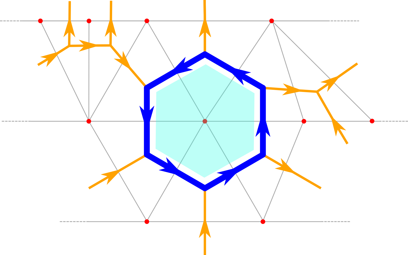
Figure 1: Sketch of a plaquette on a section of a typical 2D CDT triangulation with vertices (red dots) causally organized in “foliae” with Euclidean time increasing vertically. For simplicity, we have considered a plaquette around a vertex with zero curvature, i.e., $n_{b}=6$, but, in principle, any number of links from $4$ to $\infty$ is allowed. Even if drawn differently, due to the representation on a plane, all triangles in this and the following figures should be considered equilateral. Taken from [18].

For any dimension $d$, the form of the plaquette action over a triangulation $\mathcal{T}$ can be written as follows

$$S_{\text{YM}}[\mathcal{T};\Phi]\equiv-\beta\!\!\!\!\sum\limits_{b\in\mathcal{T}^{(d-2)}}\!\!\frac{1}{n_{b}}\Big{[}\frac{1}{N}ReTr\Pi_{b}-1\Big{]},$$ (3)

where the sum is over all $(d-2)$-simplexes of the triangulation $\mathcal{T}^{(d-2)}$, $\Pi_{b}$ is the oriented product of link variables around $b$ (i.e., the plaquette) and $n_{b}$ is the plaquette length, which, in turn, is proportional to the area inside the plaquette. Notice that $\beta$ is proportional to $1/g^{2}$ with a non-universal factor depending on the discretization and it would in general differ even in the flat case for square, hexagonal or kagome lattices. More details on the choice of the dual lattice instead of the direct one, and about the presence of the weight $\frac{1}{n_{b}}$, can be found in the original paper [18].

3 Outline of the algorithm in 2D

While the expression stated above are valid in any dimension, here we briefly describe the algorithmic setup by specializing the discussion to the 2D case.

The path-integral over configurations of the composite system can be computed by a Monte Carlo sampling of the discretized distributions $\exp(-S_{\text{CDT}}^{(\text{2D})}-S_{\text{YM}})$, where the Yang-Mills action takes the form in eq. (3), while the CDT action in two dimensions is simply [5]

$$S_{\text{CDT}}^{(\text{2D})}[\mathcal{T}]=\lambda N_{2}[\mathcal{T}],$$ (4)

where $N_{2}[\mathcal{T}]$ is the number of triangles in the triangulation $\mathcal{T}$ (i.e., the total volume), and $\lambda$ is the only free parameter, which is related to the cosmological constant.

In pure gravity CDT, simulations proceed by Metropolis–Hastings steps [19, 20] which locally change the triangulations by keeping the causal structure intact: the set of causal ergodic moves usually adopted in CDT are called Alexander moves [21, 22]. In two dimensions, these moves are the flip of a time-like link, denoted by $(2,2)$, and the creation (or destruction) of a vertex, denoted $(2,4)$ and $(4,2)$, where the notation follows the number of triangles involved before and after the move; these are depicted in figures 2 and 3 for the underlying triangulation (red dots and grey lines). In the composite gravity-gauge case, any change in the geometry $\mathcal{T}\to\mathcal{T}^{\prime}$ would also affect also the space of gauge configurations, in such a way that we need to define a map $\mathcal{C}_{G}\big{(}\mathcal{T}\big{)}\to\mathcal{C}_{G}\big{(}\mathcal{T}^{\prime}\big{)}$ between spaces of possibly different numbers of dimensions. For example, in the $(2,4)$ move (or its inverse), shown in figure 3, a plaquette is created (or destroyed), and this fact reflects non-trivially on the detailed balance condition. Also the $(2,2)$ move, depicted in figure 2, contributes with a non-zero action variation because the $\frac{1}{n_{b}}$ term in equation (3) changes for all of the four plaquettes involved.

Of course, for moves changing the triangulation, the map $\mathcal{C}_{G}\big{(}\mathcal{T}\big{)}\to\mathcal{C}_{G}\big{(}\mathcal{T}^{\prime}\big{)}$ can be chosen arbitrarily, but, for performance reasons, it is useful to keep the acceptance rate high enough by making only minimal local changes to the gauge fields. Another tool, that proves to be quite useful in the detailed balance analysis, is the freedom to gauge transform configurations within the same gauge orbit: this way, it is possible to gauge fix some link variables to the group identity, greatly simplifying the expressions involved, as shown in figures 2 and 3.

Finally, one has also to guarantee ergodicity within the space of gauge field configurations $\mathcal{C}_{G}\big{(}\mathcal{T}\big{)}$ on a fixed triangulation $\mathcal{T}$. This can be done in analogy to standard Yang–Mills simulations, where one changes just the value of a link variable usually via heat-bath sampling as in figure 4, recalling that staples can have an arbitrary length in this case.

More details on the detailed balance analysis and the sampling strategy can be found in the appendix of [18].

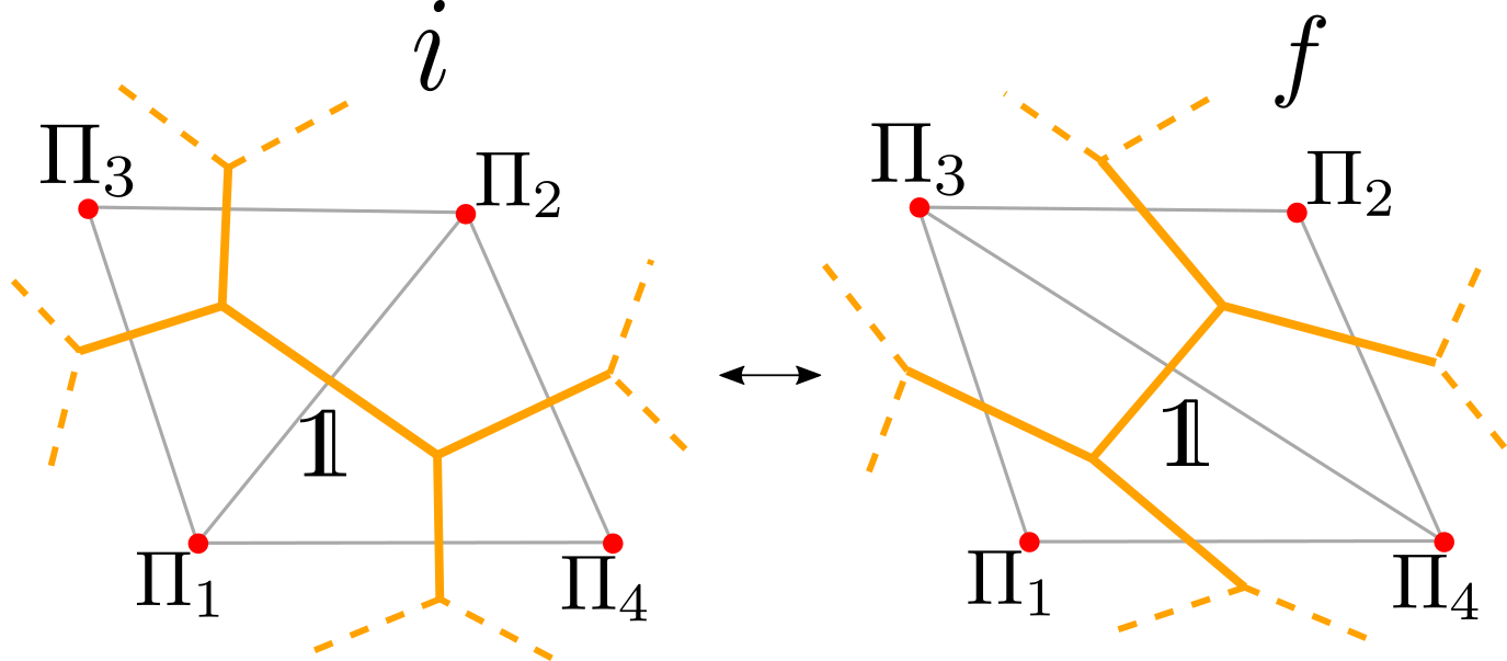
Figure 2: Sketch of a $(2,2)$ move. The edge dual to the flipped link is gauge fixed to the identity. Notice that, even if the plaquettes involved $\Pi_{1\leq i\leq 4}$ keep the same value after the move, their contribution to the action does change because the coordination numbers of all the four involved vertices change. Taken from [18].

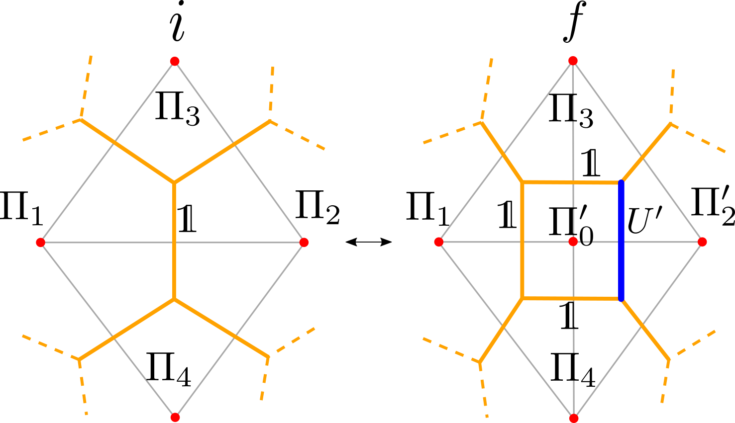
Figure 3: Sketch of a $(2,4)$ move and its inverse. The link variable $U^{\prime}$ (in blue) is the newly extracted one. Taken from [18].

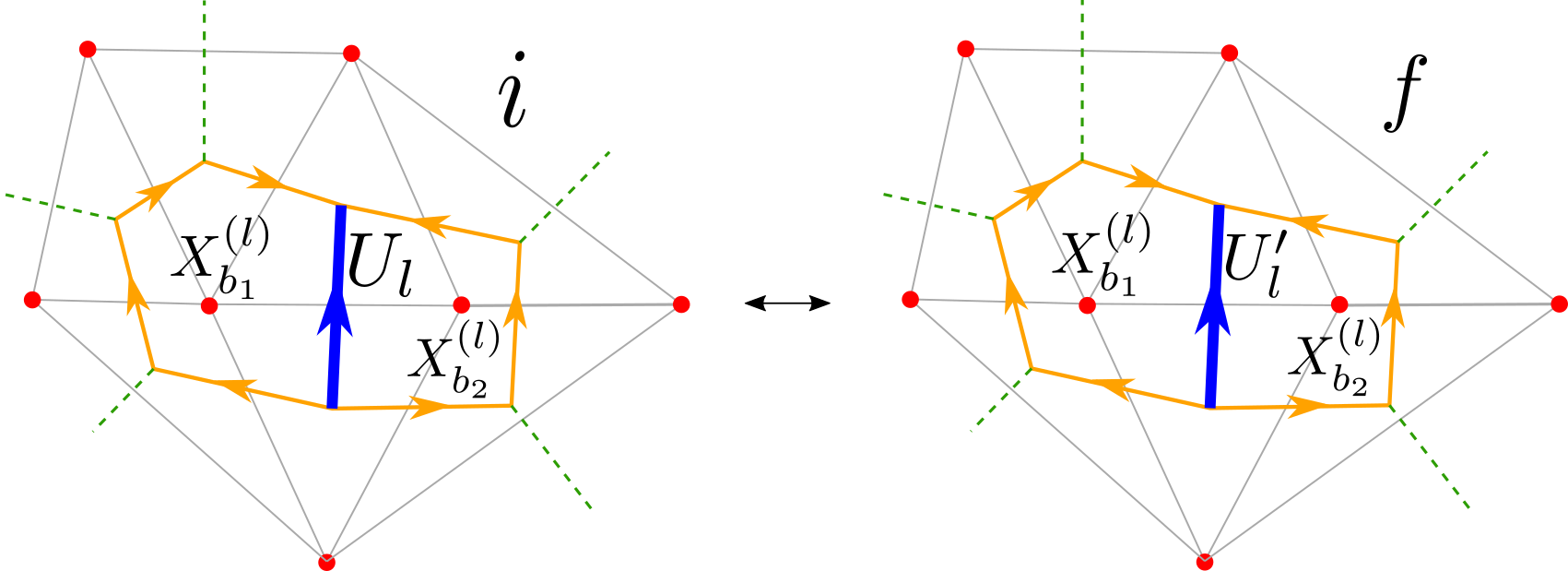
Figure 4: Sketch of a typical gauge move. The initial and final state change only in the value of the link variable associated to the edge $l$ (in blue) of the graph dual to the triangulation. The staples $X^{(l)}_{b_{1}}$ and $X^{(l)}_{b_{2}}$ are built as product of link variables oriented as indicated by the arrows (the orange paths). Taken from [18].

4 Numerical Results

In this Section we report some of the numerical results obtained in [18] for $U(1)$ and $SU(2)$ gauge theories minimally coupled to CDT in 2 dimensions.

Before showing the results, we briefly mention the parameters involved in the discretization and the numerical setup: on the gravity side the bare coupling $\lambda$ acts as a cosmological parameter in front of the total volume, since the path-integral is weighted by $\exp(-\lambda V)$; in this respect, $\lambda$ can be interpreted as a chemical potential coupled to the total volume $V$: lowering its value results in an increase of the average volume $\langle V\rangle$, up to a certain critical value $\lambda_{c}$ below which the average volume is diverging. For two dimensional CDT, this treshold has been computed exactly by analytical means and has the value $\lambda_{c}^{(0)}=\log(2)\simeq 0.693147$ (see Refs. [23, 24, 5]). In general, close to the critical point, we expect not only the average volume, but also other observables to present a critical behavior which can be fitted to a power law scaling of the form:

$$f(\lambda)=\frac{A}{{(\lambda-\lambda_{c})}^{\alpha}},$$ (5)

where $\alpha$ is the critical index associated to the observable. Another parameter is the number of time slices $N_{t}$, which is fixed and constant throughout the simulation (since it is kept unchanged by Alexander moves); we fixed it in such a way that one could neglect finite size effects, which could be assessed by measuring the two point correlations functions in the time direction for either gravity or gauge related observables (these will be introduced in the subsections). Furthermore, for simplicity, we chose the topology of triangulations to be periodic in both the time and space directions. On the gauge field side, the only parameter is inverse gauge coupling $\beta\propto 1/g^{2}$, defined in eq. (3), so that for the composite gravity-gauge theory one expects in general some dependence on $\beta$ of the critical value $\lambda_{c}=\lambda_{c}(\beta)$, below which the average volume diverges.

4.1 Gravity related observables

To characterize the gravity part of the system, we have considered two observables: the total volume of the triangulation $V\equiv N_{2}$ (i.e., the total number of triangles) and the volume profiles, i.e., the number of spatial links (spatial edges of the triangles) $V(t)\equiv N_{1s}(t)$ in each slice, where $t$ labels the slice time. From the volume profiles one can derive its associated two-point correlation function, defined as

$$C_{\text{Vprof.}}(\Delta t)\equiv\frac{\langle V(t)V(t+\Delta t)\rangle-\langle V(t)\rangle\langle V(t+\Delta t)\rangle}{\langle V(t)^{2}\rangle-\langle V(t)\rangle^{2}},$$ (6)

which, at least for $\Delta t\ll N_{t}$, is expected to decay exponentially as $\exp{\big{(}-\frac{\Delta t}{\xi_{\text{Vprof}}}\big{)}}$, where $\xi_{\text{Vprof}}$ denotes the correlation length of volume profiles.

For $\beta=0$, the Yang-Mills part of the action does not contribute at all, so the results for gravitational observables are expected to follow exactly the same behavior as in the case without gauge fields, $\lambda_{c}(0)=\log(2)$. For $\beta>0$, there is some effect of gauge fields on the gravity side; for example, a fit of the correlation length of volume profiles $\xi_{\text{Vprof}}$ to a shifted power-law behavior (eq. (5)) from simulations with gauge group $U(1)$ at $\beta=1$ gives the estimate $\lambda_{c}^{(G)}=0.6064(2),\ \nu=0.53(3)$ ($\chi^{2}/{\rm dof}=8.6/13$).

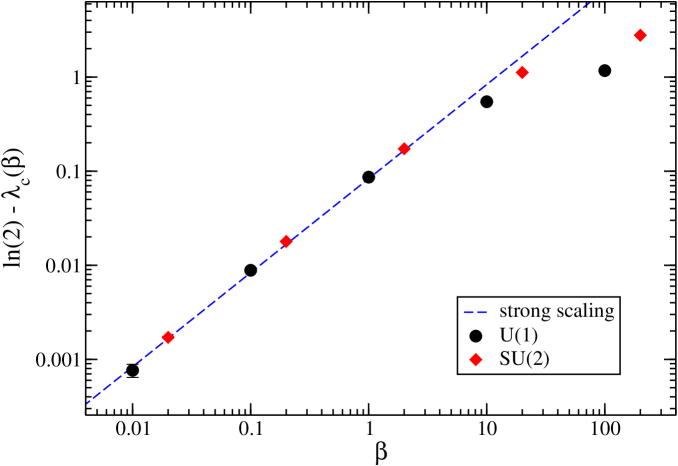
Figure 5: Critical points for the $U(1)$ and $SU(2)$ gauge theories minimally coupled to two-dimensional CDT as a function of $\beta$. Taken from [18].

Notice that the critical value is shifted a slightly below the value of the pure gravity theory $\lambda_{c}(0)=\log 2$: this is observed for a wide range of $\beta$ considered, as shown in figure 5, where we report the quantity $\log 2-\lambda_{c}^{(G)}(\beta)$ for the two gauge groups $G=U(1)$ and $G=SU(2)$. Furthermore, for $\beta\lesssim 1$, the data follows quite well the scaling $\lambda_{c}^{(G)}(\beta)=\log(2)-\beta/12$, which can be expected from a strong coupling argument (see [18]).

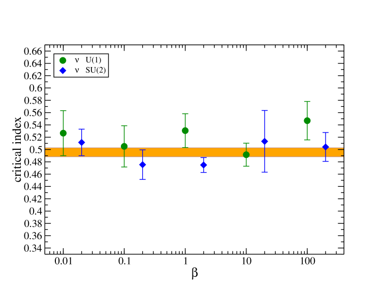
Figure 6: Critical index $\nu$ for the correlation length of volume profiles $\xi_{\text{Vprof.}}$ (see eq. (5)), plotted as a function of the bare gauge coupling $\beta$. The horizontal bands represent the results of a fit to constant values discussed in the text. Taken from [18].

Regarding the critical index $\nu$ (associated to $\xi_{\text{Vprof}}$), figure 6 shows its value for both groups considered and for a wide range of the gauge parameter $\beta$: it is interesting that $\nu$ appears to be independent of $\beta$ in the whole range, suggesting that the only effects of the gauge fields on gravity observables consist in a shift of $\lambda_{c}$, which, being not observable, can be interpreted just as a reparametrization of the bare cosmological parameter. On the basis of the apparent stability observed, we have performed a fit of all determinations to a constant value, obtaining $\nu=0.496(7)$ ($\chi^{2}/\textrm{dof}=9.1/9$), which is compatible with the value expected in the pure gravity case ($\nu=\frac{1}{2}$) (see [23, 24, 5, 25]).

4.2 Gauge observables

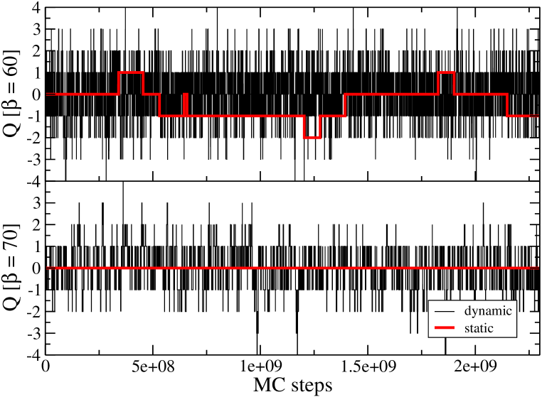
Figure 7: Comparison of topological charge histories at $\beta=60$ and $70$ for the static (flat) and dynamic simulations at average volume $N_{2}=800$ and with $N_{t}=20$ slices. Taken from [18].

An interesting observable for the gauge part of geometries with toroidal topology is the topological charge, which acts as a winding number for the gauge field and is integer-valued only for the $U(1)$ gauge group. On a 2D lattice, this can be discretized as

$$Q\equiv\frac{1}{2\pi}\sum_{b\in\mathcal{T}^{(0)}}\arg[Tr(\Pi_{b})],$$ (7)

where $\Pi_{b}$ is the plaquette around the vertex $b$, and the argument function $\arg z$ has image in the interval $(-\pi,\pi]$. From the distribution of the topological charge, one can derive its cumulants, which are related to the expansion of the free energy density $f$ of the gauge theory in powers of the topological parameter $\theta$. In particular the topological susceptibility, $\chi\equiv\langle Q^{2}\rangle/V$, fixes the leading order quadratic dependence, $f(\theta)=\chi\theta^{2}/2+O(\theta^{4})$.

A typical behavior of the topological charge for two values of $\beta$ ($60$ and $70$) is shown in Figure 7, where we also compare it with an analogous simulation on an static flat hexagonal lattice with the same total volume, where the infamous topological freezing [26, 27, 28, 29] at large $\beta$s is quite evident.

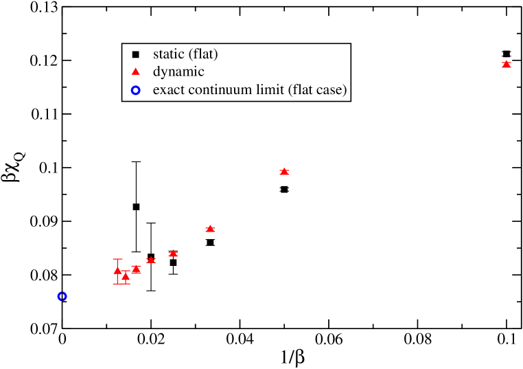
Figure 8: Comparison in topological susceptibilities for the static (flat) and dynamic simulations at average volume $N_{2}=800$ and $N_{t}=20$ slices. Taken from [18].

This mitigation to the topological freezing in the curved dynamical case, allows us to obtain an accurate estimation of the susceptibility even at values of $\beta$ difficult to reach in the static flat case, as shown in figure 8; here, one can observe a slight difference between the case with and without gravity, suggesting the presence of some physical effect of gravity on the gauge fields. Furthermore, it is also possible to extrapolate (fitting at $\beta>30$) the value of the susceptibility at $\beta\to\infty$, which turns out to be $\beta\chi_{Q}=0.0758(14)$ with a reduced chi-squared $\chi^{2}/\textrm{dof}=1.6/3$: this appears to be in agreement with the analytical prediction for the flat continuum theory [30], which, taking into account the additional factor 6 in our definition of $\beta$, is $\beta\chi_{Q}=3/(4\pi^{2})$. However, the limit $\beta\to\infty$ is naiv̈e and not sufficient in the investigation of the continuum limit of the composite theory, which depends also on the $\lambda$ parameter. As briefly mentioned in the conclusions, for a consistent continuum limit analysis, one should introduce another independent scale besides the correlation length of volume profiles. To this extent, we also considered the connected two point correlation functions of torelonic profiles, defined as:

$$C_{\text{tor}}(\Delta t)\equiv\frac{\langle Tr\Pi(t)Tr\Pi^{\dagger}(t+\Delta t)\rangle-|\langle Tr\Pi(t)\rangle|^{2}}{\langle|Tr\Pi(t)|^{2}\rangle-|\langle Tr\Pi(t)\rangle|^{2}}\,,$$ (8)

from which one can extract as before the corresponding correlation length $\xi_{\text{tor.}}$.

5 Discussion and Conclusions

We discussed the numerical implementation of compact gauge fields minimally coupled to CDT as link variables attached to edges of the graphs dual to triangulations. In our numerical analysis, we first studied gravity related observables, namely the total volume and the volume profiles; while the critical value of the bare cosmological coupling $\lambda$ is $\lambda_{c}=\log(2)$ in the pure gravity case, the value of $\lambda_{c}(\beta)$ found for the system coupled to gauge fields with a finite bare gauge coupling $\beta$ seems to be shifted below $\log(2)$, and, for small $\beta$, it follows quite well a strong coupling estimate. In particular, the critical index $\nu$ associated with the correlation length of volume profiles is found to be independent of $\beta$ within errors, and a fit to a constant function gives the estimate $\nu=0.496(7)$, i.e. $\nu$ is compatible with the analytical prediction obtained in the pure gravity theory. These observations suggest that, besides an unobservable shift in its bare parameter, gravity is not influenced by gauge fields; this could signal that gauge fields may be actually integrated away in this case as it happens also in other two dimensional contexts (see, e.g., the discussion in Refs. [31, 32, 33, 30]).

On the other hand, the gauge fields dynamics seems to be affected by the coupling with gravity in a less trivial way. In the case of the $U(1)$ gauge group in 2D, we can study the dependence of the free energy on the topological parameter $\theta$ via measurements of the integer valued topological charge. For generic gauge groups, an interesting quantity to measure is the torelon correlator and its associated correlation length in slice time, which is physically independent from the correlation length of volume profiles and could therefore be used as a distinct length scale in the analysis of the continuum limit.

Indeed, as future developments to this exploratory study, we plan to investigate, in the region of the $\lambda-\beta$ plane close to the critical line, the so-called curves of constant physics, along which the ratio between the two types of correlation lengths is fixed to a value that, in principle, could identify different physical theories in the continuum limit. Moreover, in the future we also plan to consider higher dimensions and coupling fermionic variables, both of which pose some algorithmic challenges.

References

- [1] S. Weinberg, General Relativity, an Einstein Centenary Survey, ch.16 Cambridge Univ. Press (1979).
- [2] M. H. Goroff and A. Sagnotti, Phys. Lett. B 160, 81-86 (1985)
- [3] M. Reuter and F. Saueressig, New J. Phys. 14, 055022 (2012)
- [4] J. Ambjorn, J. Jurkiewicz and R. Loll, A Nonperturbative Lorentzian path integral for gravity, Phys. Rev. Lett. 85 (2000) 924 [arXiv:hep-th/0002050 [hep-th]].
- [5] J. Ambjorn, A. Goerlich, J. Jurkiewicz and R. Loll, Nonperturbative Quantum Gravity, Phys. Rept. 519 (2012) 127 [arXiv:1203.3591 [hep-th]].
- [6] R. Loll, Quantum Gravity from Causal Dynamical Triangulations: A Review, Class. Quant. Grav. 37 (2020) 013002 [arXiv:1905.08669 [hep-th]].
- [7] J. Ambjorn, J. Jurkiewicz and R. Loll, Dynamically triangulating Lorentzian quantum gravity, Nucl. Phys. B 610 (2001) 347 [arXiv:hep-th/0105267 [hep-th]].
- [8] T. Regge, General Relativity Without Coordinates, Nuovo Cim. 19 (1961) 558.
- [9] E. Minguzzi and M. Sanchez, The Causal hierarchy of spacetimes, [arXiv:gr-qc/0609119 [gr-qc]].
- [10] J. Ambjorn, S. Jordan, J. Jurkiewicz and R. Loll, A Second-order phase transition in CDT, Phys. Rev. Lett. 107 (2011) 211303 [arXiv:1108.3932 [hep-th]].
- [11] J. Ambjorn, S. Jordan, J. Jurkiewicz and R. Loll, Second- and First-Order Phase Transitions in CDT, Phys. Rev. D 85 (2012) 124044 [arXiv:1205.1229 [hep-th]].
- [12] J. Ambjørn, J. Gizbert-Studnicki, A. Görlich, J. Jurkiewicz, N. Klitgaard and R. Loll, Characteristics of the new phase in CDT, Eur. Phys. J. C 77 (2017) 152 [arXiv:1610.05245 [hep-th]].
- [13] J. Ambjorn, D. Coumbe, J. Gizbert-Studnicki, A. Gorlich and J. Jurkiewicz, New higher-order transition in causal dynamical triangulations, Phys. Rev. D 95 (2017) 124029 [arXiv:1704.04373 [hep-lat]].
- [14] J. Ambjørn, J. Gizbert-Studnicki, A. Görlich, K. Grosvenor and J. Jurkiewicz, Four-dimensional CDT with toroidal topology, Nucl. Phys. B 922 (2017) 226 [arXiv:1705.07653 [hep-th]].
- [15] J. Ambjørn, J. Gizbert-Studnicki, A. Görlich, J. Jurkiewicz and D. Németh, The phase structure of Causal Dynamical Triangulations with toroidal spatial topology, JHEP 06 (2018) 111 [arXiv:1802.10434 [hep-th]].
- [16] G. Clemente and M. D’Elia, Spectrum of the Laplace-Beltrami operator and the phase structure of causal dynamical triangulations, Phys. Rev. D 97 (2018) 124022 [arXiv:1804.02294 [hep-th]].
- [17] G. Clemente, M. D’Elia and A. Ferraro, Running scales in causal dynamical triangulations, Phys. Rev. D 99 (2019) 114506 [arXiv:1903.00430 [hep-th]].
- [18] A. Candido, G. Clemente, M. D’Elia and F. Rottoli, JHEP 04, 184 (2021) [arXiv:2010.15714 [hep-lat]].
- [19] N. Metropolis, A. W. Rosenbluth, M. N. Rosenbluth, A. H. Teller and E. Teller, Equation of state calculations by fast computing machines, J. Chem. Phys. 21 (1953) 1087
- [20] W. K. Hastings, Monte Carlo Sampling Methods Using Markov Chains and Their Applications, Biometrika 57 (1970) 97
- [21] J.W. Alexander, The combinatorial theory of complexes, Ann. Mat. 31 (1931) 292.
- [22] J. Ambjørn, J. Jurkiewicz and R. Loll, Lorentzian and Euclidean Quantum Gravity — Analytical and Numerical Results, NATO Sci. Ser. C 556 (2000) 381 [arXiv:hep-th/0001124 [hep-th]].
- [23] J. Ambjorn and R. Loll, Nonperturbative Lorentzian quantum gravity, causality and topology change, Nucl. Phys. B 536 (1998) 407 [arXiv:hep-th/9805108 [hep-th]].
- [24] J. Ambjorn, R. Loll, J. L. Nielsen and J. Rolf, Euclidean and Lorentzian quantum gravity: Lessons from two-dimensions, Chaos Solitons Fractals 10 (1999) 177 [arXiv:hep-th/9806241 [hep-th]].
- [25] S. Zohren, [arXiv:hep-th/0609177 [hep-th]].
- [26] B. Alles, G. Boyd, M. D’Elia, A. Di Giacomo and E. Vicari, Hybrid Monte Carlo and topological modes of full QCD, Phys. Lett. B 389 (1996) 107 [arXiv:hep-lat/9607049 [hep-lat]].
- [27] L. Del Debbio, G. M. Manca and E. Vicari, Critical slowing down of topological modes, Phys. Lett. B 594 (2004) 315 [arXiv:hep-lat/0403001 [hep-lat]].
- [28] M. Luscher and S. Schaefer, Lattice QCD without topology barriers, JHEP 07 (2011) 036 [arXiv:1105.4749 [hep-lat]].
- [29] C. Bonati and M. D’Elia, Topological critical slowing down: variations on a toy model, Phys. Rev. E 98 (2018) 013308 [arXiv:1709.10034 [hep-lat]].
- [30] C. Bonati and P. Rossi, Topological susceptibility of two-dimensional gauge theories, Phys. Rev. D 99 (2019) 054503 [arXiv:1901.09830 [hep-lat]].
- [31] J. Ambjorn and A. Ipsen, Phys.Rev.D 88 (2013) 6 [arXiv:1305.3148 [hep-th]].
- [32] J. Ambjorn, K. N. Anagnostopoulos and J. Jurkiewicz, Abelian gauge fields coupled to simplicial quantum gravity, JHEP 08 (1999) 016 [arXiv:hep-lat/9907027 [hep-lat]].
- [33] C. Cao, M. van Caspel and A. R. Zhitnitsky, Topological Casimir effect in Maxwell Electrodynamics on a Compact Manifold, Phys. Rev. D 87 (2013) 105012 [arXiv:1301.1706 [hep-th]].