The $D_{s}DK^{*}$ vertex in QCD Sum Rules: form factors and coupling constant

Abstract

In this work we study the meson vertex $D_{s}DK^{*}$ using the QCD sum rules. We compute the three point correlation functions for the three cases of different off-shell mesons. The form factors for each case are fitted to the numerical calculation of the correlation functions and the coupling constant of the vertex is obtained by comparing the form factors at their respective off-shell meson pole. The result obtained for the coupling constant is $g_{D_{s}DK^{*}}=2.29^{+0.65}_{-0.41}$.

I Introduction

The study of hadrons has widely improved by the efforts of many experimental collaborations such as Belle (KEK, Japan), BaBar (SLAC, USA), BESIII (BEPCII, China), CDF and LHCb (LHC, Switzerland), that have been collecting a large amount of experimental data in the last decades. These data have become a remarkable testing ground for different approaches that deal with the non-perturbative nature of the strong interactions between hadrons in decay processes. The calculation of the cross sections of the decay processes can be used to elucidate a little more about the complex world of the fundamental particles interactions. In order to study these hadronic decay processes, it is necessary to address the large theoretical challenge of the non-perturbative nature of Quantum Chromodynamics (QCD). The QCD, the fundamental theory of the strong interactions between quarks and gluons, is non-perturbative at low energies since its coupling constant $\alpha_{s}(q^{2})$ increases as $|q^{2}|$ decreases. Therefore, it is necessary to use some non-perturbative approaches like some effective field theories. One of the more usual approach used is based in the effective $SU(4)$ lagrangian, [1, 2, 3], where the quarks $u$, $d$, $s$ and $c$ are considered to have the same mass. With this effective theory, it is possible to perform the theoretical cross section, where two fundamental ingredients are needed, one is the form factor and the other is the coupling constant of the vertex. The form factor is responsible to carry the unknown non-perturbative dynamics of the strong interactions. It is represented by a function of the squared momentum, $g(q^{2})$, and is not always directly observed experimentally. For this reason, the shape of the form factor used has the same shape as low energy nuclear physics, where only the parameters need to be adjusted. The situation is similar for the coupling constants, there is not, in general, experimental data that permit to infer their values. One exception is the coupling constant of the $D^{*}D\pi$ decay, where through the width of $D^{*}$, the decay coupling constant was calculated [4]. But in other cases, the coupling constant would be obtain using the relations of the $SU(4)$ [1].

Our group had been improving a method to calculate the form factors and coupling constants, in some charmed and botton decays, using a non-perturbative approach called Quantum Chromodynamics Sum Rules (QCDSR). The QCDSR technique was developed by the authors Shifman, Vainshtein and Zakharof [5, 6]. It is a powerful and analytical tool that allow us to compute the physical properties of hadrons, such as the masses, decay constants, form factors and coupling constants. We have been studying, for a long time, a technique to obtain form factors and coupling constant and improve the results with less uncertainties. Some of our three mesons strange-charmed vertices that were calculated are: $J/\psi D_{s}D_{s}$ [7], $J/\psi D_{s}^{*}D_{s}^{*}$ [8], $\eta_{c}D^{*}D$ and $\eta_{c}D_{s}^{*}D_{s}$ [9], $D_{s}D_{s}\phi$ [10], $D^{*}D_{s}K$ and $D^{*}_{s}DK$ [11], the $B_{s}B^{*}K$ [12] , the $B_{s}B^{*}K$ and $B_{s}BK^{*}$ [13], and many other that can be seen in Ref. [1].

Our method consists of calculating, for the three meson decay, three different form factors that are obtained when each meson is used as a projectile of the vertex (the target). In this way, we obtain information about how each particle ”reads” the interaction vertex. But each form factor, $g_{i}(q^{2})$, may give the same value for the coupling constant, which could be obtained when $q^{2}\to m^{2}_{\rm{off}}$, where $m_{\rm{off}}$ is the mass of the off-shell meson. This is possible when we work in the QCDSR respecting the stability of the sum rule. The details of our approach and the earlier results are reviewed in Ref. [1]. In that review, it is noted that the shape of the form factors in several charmed decay processes present some regularity, related to the shape of the function that represent the form factor.

Following up our studies of vertices with open charm mesons, our objective in the present work is to apply our method to study the form factors and the coupling constant of the vertex $D_{s}DK^{*}$. In a previous work, the vertices $D^{*}D_{s}K$ and $DD_{s}^{*}K$ were calculated [11]. These vertices are important in studies of the dissociation cross section of $J/\psi$ by kaons, and the suppression of the charmonium production is an important signature of the quark-gluon plasma (QGP) in heavy ion collisions. Another important type of processes that these vertices plays a role are decays with final state interactions (FSI), in which a meson decays into an intermediate state, and then the mesons of the intermediate state interact via particle exchange, before decaying into the final state. One example of such process is the $B^{\pm}\to DD_{s}\to K^{*}\pi^{\pm}$, shown in Fig. (1). This decay is important because it can be used to detect direct CP violation and to determine the CKM parameters mixing. Note that the vertex $BDD_{s}$ represents an effective electroweak interaction, so it can be evaluated by the Hamiltonian of the electroweak theory [14].

Figure 1: FSI decay process $B\to DD_{s}\to K^{*}\pi$.

Considering that the vertex $D_{s}DK^{*}$ has three distinct mesons, each one of them can act as the projectile. Therefore, it is necessary to take this into account and compute the three-point correlation function for all the possible cases, obtaining three different form factors and coupling constants. Given that the coupling constant must be the same regardless of which meson is off-shell, the mean value of the three calculated couplings will result in a single value for the coupling constant of the vertex. This procedure gives a more reliable result, since there is no reason to choose only one of three possible form factors to determine the coupling constant. Besides that, an important source of uncertainty in the numerical calculation originates from the fact that the QCDSR results are reliable on a small window of momentum, with $Q^{2}>0$, and the coupling constant is obtained from the value of the form factor at the off-shell meson pole, $g=g(Q^{2}=-m_{\rm{off}}^{2})$ (i.e. at $Q^{2}<0$), meaning that the results have to be fitted in this small window and then be extrapolated to a range of momentum outside the window which the sum rules calculations are actually performed. Therefore, by calculating all the possible off-shell cases, the uncertainties regarding this extrapolation are also minimized by the procedure, as the three coupling constants calculated must converge to a single value (considering their error bars).

This paper is organized as follows: in section II, we show the calculation of the three-point correlation function of the vertex $D_{s}DK^{*}$; in section III, we present the final equations of the sum rule for each off-shell case; the numerical analysis and results are discussed in section IV; our final remarks and conclusion are on section V, where we also compare our results with previous calculations found in literature.

II The three point correlation function

The main element of the QCDSR technique is the correlation function, such as the two-point correlation function that can be used to obtain the mass of the hadron, and the three-point function used to obtain the form factors and coupling constants. The quark-hadron duality principle states that hadrons can be described equally by the quarks and gluons degrees of freedom and also by the hadronic degrees of freedom. Thus the correlation function can be computed in two different ways: on the OPE side (or QCD side), the quark and gluons fields are used; and on the phenomenological side the hadronic ones are used. When comparing both sides of the sum rule, it is possible to obtain an equation for the physical parameters that are introduced on the phenomenological side.

The three-point correlation function for the vertex $D_{s}DK^{*}$, with the off-shell meson $M=D_{s},D,K^{*}$, is written as:

$$\Gamma_{\mu}^{(M)}=\int d^{4}x\,d^{4}y\,e^{ip^{\prime}\cdot x}\,e^{-iq\cdot y}\langle 0|T{j_{1}(x)j_{2}^{\dagger}(y)j_{3}^{\dagger}(0)}|0\rangle,$$ (1)

where the relation between the mesons four momentum is $q=p^{\prime}-p$, and the functions $j_{i}$ are meson interpolating currents that represent the mesons in terms of quarks degrees of freedom, when it is computed by the QCD side.

The order of the currents on the correlator of Eq. (1) depends on the mesons configuration in the vertex [15, 16]. We will study the three possible cases of off-shell mesons for this vertex – $D$, $D_{s}$ and $K^{*}$ off-shell – as shown in Fig. (2).

(a) $D$ off-shell

(b) $D_{s}$ off-shell

(c) $K^{*}$ off-shell

Figure 2: The $D_{s}DK^{*}$ vertex with off-shell mesons.

For this vertex, we need the following currents that contain the quantum properties of the mesons written in terms of quark fields:

$$j_{\mu}^{K^{*}} = \bar{u}\gamma_{\mu}s,$$

$$j^{D}_{5} = i\bar{c}\gamma_{5}q,$$

$$j^{D_{s}}_{5} = i\bar{c}\gamma_{5}s,$$ (2)

where $q$ is the up or down quark, $c$ is the charm and $s$ is the strange quark.

On the OPE side of the sum rule, the correlation function is calculated by the input of the interpolating currents from Eq. (2) into the Eq. (1), and then a Wilson operator product expansion (OPE) is carried out. Here, the time ordered product of the local currents is expanded in terms of local operators and incorporates the non-perturbative effects corrections in the sum rule. These operators are ordered in terms of increasing dimension: the first one is the unitary operator for the perturbative contribution; the next ones are non-perturbative contributions composed by quarks and gluons fields and their QCD vacuum expectation values, known as the condensates of quarks and gluons.

Using the Cutkosky’s rule, the correlation function can be written as a double dispersion relation, for the different Dirac structures present in the function:

$$\Gamma_{\mu}^{\rm OPE}(p^{2},p^{\prime 2},q^{2})=-\frac{1}{4\pi^{2}}\int_{0}^{\infty}\int_{0}^{\infty}ds\,du\frac{\rho_{\mu}^{\rm OPE}(s,u,q^{2})}{(s-p^{2})(u-p^{\prime 2})},$$ (3)

where the function $\rho_{\mu}^{\rm{OPE}}$ is the spectral density that is related to the double discontinuity of the amplitude. The spectral densities are computed at first order of the perturbative expansion in $\alpha_{s}$, the strong coupling constant. The OPE in this work includes terms up to dimension five of the condensates, leading to the following OPE side of the sum rule:

$$\Gamma_{\mu}^{\rm OPE}=\Gamma_{\mu}^{\rm pert}+\Gamma_{\mu}^{\langle\bar{q}q\rangle}+\Gamma_{\mu}^{m_{s}\langle\bar{q}q\rangle}+\Gamma_{\mu}^{\langle g_{s}^{2}G^{2}\rangle}+\Gamma_{\mu}^{\langle\bar{q}Gq\rangle}+\Gamma_{\mu}^{m_{s}\langle\bar{q}Gq\rangle},$$ (4)

where $q$ is a quark up, down or strange, $\Gamma_{\mu}^{\rm pert}$ is the perturbative term of the OPE, the following terms are the non-perturbative contributions from quarks $\langle\bar{q}q\rangle$, gluons $\langle g_{s}^{2}G^{2}\rangle$ and mixed condensates $\langle\bar{q}Gq\rangle$ and $m_{s}$ mass corrections.

On the phenomenological side of the sum rule, the correlation function of Eq. (1) is interpreted in terms of meson currents that creates and annihilates the hadronic states of the vertex. This is done by inserting the intermediate hadronic states in Eq. (1). The matrix elements thus obtained are written in terms of the hadronic physical parameters – the masses and decay constants:

$$\langle 0|j_{D}|D(p_{a})\rangle=\frac{m_{D}^{2}f_{D}}{m_{c}+m_{u}}\,,$$

$$\langle 0|j_{D_{s}}|D_{s}(p_{b})\rangle=\frac{m_{D_{s}}^{2}f_{D_{s}}}{m_{c}+m_{s}}\,,$$

$$\langle 0|j_{\mu}^{K^{*}}|K^{*}(p_{c},\epsilon)\rangle=m_{K^{*}}f_{K^{*}}\epsilon_{\mu}(p_{c})\,.$$ (5)

The respective mesons four momenta $p_{a}$, $p_{b}$ and $p_{c}$ can be $p$, $p^{\prime}$ or $q$, depending on which meson is off-shell, according to the Fig. (2). The vertex amplitude matrix is derived from the hadronic interaction lagrangian, which defines the coupling constant of the vertex ${D_{s}DK^{*}}$ [17]:

$$\mathcal{L}=ig_{D_{s}DK^{*}}\left[K^{*\alpha}\left(D\partial_{\alpha}\bar{D_{s}}-\bar{D_{s}}\partial_{\alpha}D\right)+\bar{K}^{*\alpha}\left(D_{s}\partial_{\alpha}\bar{D}-\bar{D}\partial_{\alpha}D_{s}\right)\right].$$ (6)

The amplitude matrices that appear in the correlation function for each off-shell meson $M$ are extracted from Eq. (6), and are given in terms of the form factors $g_{D_{s}DK^{*}}^{(M)}(q^{2})$. The resulting amplitude matrices for the $D$, $D_{s}$ and $K^{*}$ off-shell meson cases are then written respectively as:

$$\langle D(q)|K^{*}(p)D_{s}(p^{\prime})\rangle=ig_{D_{s}DK^{*}}^{(D)}(q^{2})(q_{\alpha}+p_{\alpha}^{\prime})\epsilon^{\alpha}(p)\,,$$

$$\langle D_{s}(q)|K^{*}(p)D(p^{\prime})\rangle=-ig_{D_{s}DK^{*}}^{(D_{s})}(q^{2})(q_{\alpha}+p_{\alpha}^{\prime})\epsilon^{\alpha}(p)\,,$$

$$\langle K^{*}(q)|D_{s}(p)D(p^{\prime})\rangle=-ig_{D_{s}DK^{*}}^{(K^{*})}(q^{2})(p_{\alpha}+p_{\alpha}^{\prime})\epsilon^{\alpha}(q)\,,$$ (7)

where the $g^{(M)}(q^{2})$’s functions are the respective form factors of the vertices.

III Sum rules

The vertices sum rules are lastly obtained following the quark-hadron duality principle, by which the two sides of the sum rule can be matched. The possible Dirac structures for the correlation functions of the $D_{s}DK^{*}$ vertex are $p_{\mu}$ and $p_{\mu}^{\prime}$. Matching the respective OPE and phenomenological sides of the sum rules, we obtain a sum rule for every Dirac structure of each one of the off-shell meson cases.

In order to improve the matching of the sides of the sum rule, a double Borel transformation is performed on both sides of the sum rules. This operation introduces the Borel mass parameters $M$ and $M^{\prime}$. The reason for this step in the calculation is that the Borel transformation enhances the convergence on the OPE side and suppresses higher order terms. After equating the OPE and phenomenological sides, the double Borel transformation is performed, with $P^{2}\to M^{2}$ and $P^{\prime 2}\to M^{\prime 2}$,

$$\mathcal{BB}\left[\Gamma^{\rm OPE}_{i}(P^{2},P^{\prime 2},Q^{2})\right]=\mathcal{BB}\left[\Gamma^{\rm phen}_{i}(P^{2},P^{\prime 2},Q^{2})\right],$$ (8)

where the squared mesons four momenta is in the Euclidean space, $p^{2}=-P^{2}$, $p^{\prime 2}=-P^{\prime 2}$ and $q^{2}=-Q^{2}$. The functions $\Gamma_{i}$ represent the correlation functions for each Dirac structure ($i=p_{\mu},p_{\mu}^{\prime}$).

At this point, the last step to assure the matching of both sides of the sum rules, is to introduce the threshold parameters $s_{sup}$ and $u_{sup}$ in the limits of integration on the OPE side, separating the pole from the continuum contributions. When this is done, only the pole contribution remains on both sides of the sum rule: the OPE continuum contribution cancels out with the h.r. terms (corresponding to the excited states above the pole) on the phenomenological side. The threshold parameters are defined as $s_{sup}=(m_{i}+\Delta_{i})^{2}$ and $u_{sup}=(m_{o}+\Delta_{o})^{2}$, with the masses $m_{i}$ and $m_{o}$ being the masses of the incoming and outgoing mesons of the vertex according to Fig. (2). The $\Delta_{i}$ and $\Delta_{o}$ parameters represent the gap between the pole resonances ($M=D,D_{s},K^{*}$) and their excited states. The values of the $\Delta$’s are determined by the best fit in the numerical analysis, and it is usually found to be around $0.5$ GeV.

The final expressions for the sum rules can be written by isolating the form factors in their respective equations and rewriting the phenomenological side as $\mathcal{B}\mathcal{B}[{\Gamma}^{\rm phen}_{(i)}(Q^{2})]$ $=g(Q^{2})\cdot\mathcal{B}\mathcal{B}[\widetilde{\Gamma}^{\rm phen}_{(i)}(Q^{2})]$. The resulting general expression is given bellow:

$$g_{D_{s}DK^{*}}^{(M)}(Q^{2})=\frac{-\frac{1}{4\pi^{2}}\int^{s_{sup}}_{s_{inf}}\int^{u_{sup}}_{u_{inf}}DD\left[\Gamma^{\rm pert}_{i}\right]e^{-\frac{(s+u)}{M^{2}}}dsdu+\mathcal{B}\mathcal{B}\left[\Gamma^{\rm non-pert}_{i}\right]}{\mathcal{B}\mathcal{B}\left[\widetilde{\Gamma}_{i}^{\rm phen}(Q^{2})\right]}\,.$$ (9)

for the $M=D,D_{s}$ and $K^{*}$ off-shell cases.

The non-perturbative terms of the OPE ($\Gamma^{\rm non-pert}$) correspond to the condensates contributions for each off-shell case: quark, gluon and mixed for the $D$ and $D_{s}$ off-shell cases, and only gluon condensates for the $K^{*}$ off-shell case. The expressions for the OPE terms and the limits of integration can be found in the appendix A.

We have also applied the following ansatzes for the Borel masses parameters, for the $D,D_{s}$ and $K^{*}$ off-shell, respectively:

$$M^{\prime 2}=M^{2}\frac{m^{2}_{D_{s}}-m_{c}^{2}}{m_{K^{*}}^{2}}$$ (10)

$$M^{\prime 2}=M^{2}\frac{m^{2}_{D}-m_{c}^{2}}{m_{K^{*}}^{2}}$$ (11)

$$M^{\prime 2}=M^{2}\frac{m_{D}^{2}}{m_{D_{s}}^{2}}$$ (12)

IV Results

	Parameter	Value
	$f_{K^{*}}$	$220\pm 5$ MeV
Decay constants [13, 9]	$f_{D}$	$206.7\pm 8.5\pm 2.5$ MeV
	$f_{D_{s}}$	$257.5\pm 6.1$ MeV
	$m_{K^{*}}$	$0.892$ GeV
Meson masses [18]	$m_{D}$	$1.869$ GeV
	$m_{D_{s}}$	$1.968$ GeV
	$m_{c}$	$1.27\pm 0.025$ GeV
Quark masses [18, 19]	$m_{u,d}$	$0$ GeV
	$m_{s}$	$101+29-21$ MeV
	$\left<q\bar{q}\right>$	$-(230\pm 30)^{3}\,\rm{MeV}^{3}$
Condensates [9]	$\left<s\bar{s}\right>$	$-(290\pm 15)^{3}\,\rm{MeV}^{3}$
	$\left<g^{2}G^{2}\right>$	$0.88\pm 0.16\,\rm{GeV}^{4}$
	$\left<qg\sigma G\bar{q}\right>$	$(0.8\pm 0.2)\left<q\bar{q}\right>\,\rm{GeV}^{5}$

Table 1: Physical parameters.

The values of the hadronic parameters used in the numerical calculations of the sum rules are listed on Table 1. We work with the $p_{\mu}$ structure for the $D$ and $D_{s}$ off-shell, and with the $p_{\mu}^{\prime}$ structure for the $K^{*}$ off-shell. This choice is based on which one of the structures provides the best fit for the form factors while respecting the constraints imposed by the QCDSR. We first show the OPE convergence in Fig. (3), where it is possible to observe that each term of the OPE series is smaller than the previous ones. It is also possible to check the region of stability of the total OPE series in this figure. The pole-continuum comparison is shown next in Fig. (4), establishing the region with pole dominance over the continuum contributions. From the Figs. (3) and (4), we extract the Borel mass windows, i.e., the range of values of the Borel mass in which the sum rules are reliable. The Borel window is further decreased with the fit of the form factors, that we will present next.

The Fig. (5) shows the resultant numerical calculations of the form factors from Eq. (9). The form factors were fitted to the numerical data computed as either a monopolar function,

$$g(Q^{2})=\frac{\mathcal{A}}{\mathcal{B}+Q^{2}}\,,$$ (13)

or an exponential function,

$$g(Q^{2})=\mathcal{A}\,e^{-\mathcal{B}Q^{2}}\,,$$ (14)

where the parameters $\mathcal{A,B}$ were determined by the fitting procedure. The form factors are chosen according to the best fit of each form factor to the numerical data. The results are shown in Table 2.

The $\Delta$ parameters, the Borel mass $M^{2}$, $Q^{2}$ windows and also the coupling constants results for the $M$ are shown in Table 3 for each off-shell meson case. The values are obtained by the extrapolation of the fitted curves of Table 2 to the non-Euclidean region $Q^{2}<0$, and then calculating the value of the form factor at the off-shell meson pole. The result thus obtained for the vertex $D_{s}DK^{*}$ coupling constant is taken from

$$g_{D_{s}DK^{*}}^{(M)}=g_{D_{s}DK^{*}}^{(M)}(Q^{2}=-m_{M}^{2})\,.$$ (15)

The coupling constant error bars are presented in Fig. (5). By comparing the error bars of the cases, it is possible to see that their values are compatible. The final result for the coupling constant of the vertex is taken from the mean value of the coupling constants presented in Table 3:

$$g_{D_{s}DK^{*}}=2.29^{+0.65}_{-0.41}.$$ (16)

Form factor	Structure	Type	$\mathcal{A}$	$\mathcal{B}$
$g^{(D)}_{DsDK^{*}}(Q^{2})$	$p_{\mu}$	Monopolar	109.52	45.140
$g^{(K^{*})}_{DsDK^{*}}(Q^{2})$	$p^{\prime}_{\mu}$	Exponential	1.488	0.560
$g^{(D_{s})}_{DsDK^{*}}(Q^{2})$	$p_{\mu}$	Monopolar	50.431	30.332

Table 2: Numerical results for the parametrization of the form factors.

	Off-shell meson / structure
	$D$ / $p_{\mu}$	$D_{s}$ / $p_{\mu}$	$K^{*}$ / $p^{\prime}_{\mu}$
$\Delta_{s}$ (GeV)	0.5	0.5	0.6
$\Delta_{u}$ (GeV)	0.6	0.6	0.6
$M^{2}$ (GeV2)	$\left[1.7,2.0\right]$	$\left[1.1,1.6\right]$	$\left[1.5,2.1\right]$
$Q^{2}$ (GeV2)	$\left[0.1,1.5\right]$	$\left[0.1,3.0\right]$	$\left[1.0,3.0\right]$
$g^{(M)}_{D_{s}DK^{*}}$	$2.63^{+0.23}_{-0.23}$	$1.91^{+0.20}_{-0.21}$	$2.32^{+0.62}_{-0.55}$

Table 3: Numerical results for the $\Delta$ parameters, the $M^{2}$ and $Q^{2}$ windows and coupling constant for each off-shell case.

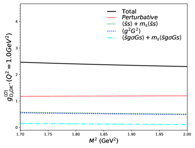
(a) $D$ meson, structure $p_{\mu}$

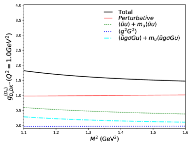
(b) $D_{s}$ meson, structure $p_{\mu}$

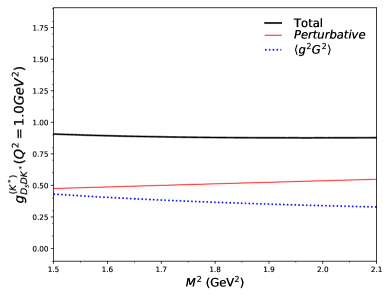
(c) $K^{*}$ meson, structure $p_{\mu}^{\prime}$

Figure 3: OPE stability and convergence, for each off-shell case and structures, with $Q^{2}=1\,$GeV².

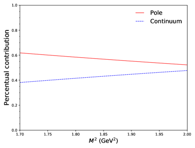
(a) $D$ off-shell, structure $p_{\mu}$

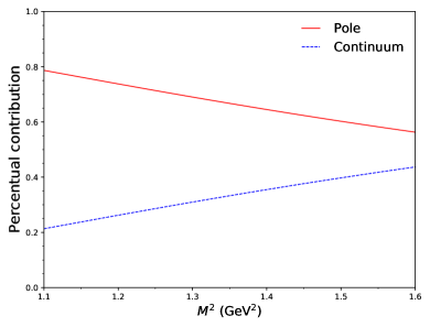
(b) $D_{s}$ off-shell, structure $p_{\mu}$

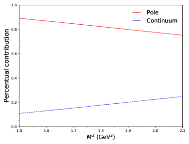
(c) $K^{*}$ off-shell, structure $p_{\mu}^{\prime}$

Figure 4: Pole-continuum contributions, for each off-shell case and structures, with $Q^{2}=1\,$GeV².

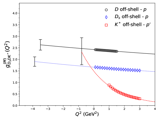
Figure 5: Form factors of the vertex $D_{s}DK^{*}$, and their respective extrapolated functions. The values of the form factor at the off-shell meson pole and the error bars are also indicated.

IV.1 Error analysis

The percentage deviations for each parameter of the QCDSR calculation are presented in Table 4. Such deviations are obtained by varying each parameter presented in the QCDSR calculation within their respective uncertainty windows, obtaining their respective coupling constants and then comparing the value of the coupling constant for each of the extremes of these windows to the values of the coupling constants presented in Table III.

In the case of decay constants, quark masses and condensates, the percentage deviations are calculated from the variation of such parameters within their respective uncertainties presented in Table I. For the parameter $Q^{2}$, we obtain the deviation by making variations of 20% in the window widths shown in Table III. For the threshold parameters ($\Delta_{s}$ and $\Delta_{u}$), we studied variations of $\pm 0.1GeV$ in each one, both separately and together. For the Borel mass $M^{2}$, we calculated the standard deviation of the coupling constant within the Borel windows shown in Table III. Finally, the deviations in the parameters of the fit functions ($\mathcal{A}$ and $\mathcal{B}$) are obtained by varying those parameters within their uncertainties indicated by the fit method itself.

The percentage deviations therefore indicate the impact that the variation of each parameter has on the calculation of the vertex coupling constant. From the Table 4, it is possible to check that the main sources of errors are the gluon condensate and the strange and charm quarks’ masses for the $K^{*}$ off-shell. For the $D$ and $D_{s}$ off-shell cases, the main sources of errors are the $\Delta$’s, the decay constant of meson $D$ and the quark condensates .

The chosen structures ($p_{\mu}$ for $M=D,D_{s}$, $p^{\prime}_{\mu}$ for $M=K^{*}$) are determined after a rigorous error analysis of the numerical fit of the form factors. The constrains on the numerical fit were the following:

• Minor global error;

• Less sensitivity to the fit, quarks masses and condensates;

• Similarity of the form factor behavior between the $D$ and $D_{s}$ off-shell cases;

• Larger as possible $Q^{2}$ window;

• Stable Borel windows;

• A convergent OPE series, with the perturbative term contribution bigger than the sum of the condensates contributions;

• Pole contribution must be bigger than the continuum contribution.

Parameter	$\Delta g_{D_{s}DK^{*}}^{(D-p)}$(%)	$\Delta g_{D_{s}DK^{*}}^{(D_{s}-p)}$(%)	$\Delta g_{D_{s}DK^{*}}^{(K^{*}-p^{\prime})}$(%)
$M^{2}$	1.18	0.55	7.67
$Q^{2}$	0.18	0.60	13.92
$\Delta_{s}\pm 0.1(GeV),\Delta_{u}\pm 0.1(GeV)$	5.44	5.83	5.78
$\left<\bar{q}g\sigma\cdot Gq\right>$	0.19	0.03	-
$\left<\bar{q}q\right>$	2.30	6.73	-
$\left<g^{2}G^{2}\right>$	2.75	0.62	7.09
$\text{Fitting Parameters }(\mathcal{A}\text{ and }\mathcal{B})$	1.42	2.51	0.82
$f_{D_{s}}$	1.94	1.94	1.94
$f_{D}$	4.35	4.35	4.36
$f_{K^{*}}$	1.85	1.85	1.85
$m_{c}$	2.02	0.93	2.31
$m_{s}$	0.83	1.17	15.44

Table 4: Percentage deviation of the coupling constants according with the variation of each parameter for the structures $p_{\mu}$ ($D$ and $D_{s}$ off-shell cases) and $p^{\prime}_{\mu}$ ($K^{*}$ off-shell).

V Summary and conclusions

In this work, the QCDSR technique was applied to perform the calculation of the form factors and coupling constant for the charmed meson vertex $D_{s}DK^{*}$. The form factors for each one of the off-shell mesons were computed, so that the uncertainties were minimized. The parametrization used for the form factors were either monopolar or exponential functions, as usual for this type of vertex. The values of the form factors at the respective off-shell meson pole mass ($Q^{2}\to-m_{\rm off}^{2}$) were combined to obtain the coupling constant of the vertex, and the final result was presented in Eq. (16).

Reference	$g_{D_{s}DK^{*}}$
This Work	$2.29^{+0.65}_{-0.41}$
SU(4) [17]	5
LCSR [20]	$1.61\pm 0.62$
QCDSR [21]	$3.26\pm 0.43$

Table 5: Comparison of the coupling constant of the vertex $g_{D_{s}DK^{*}}$ that were obtained in different works.

We can compare our results with previous calculations for the same vertex, as shown in Table 5. In Ref. [17], the $SU(4)$ estimate for the coupling constant is more than two times bigger than ours, showing a large $SU(4)$ breaking effect. In Ref. [20], the coupling constant of the vertex $D_{s}DK^{*}$ was computed in the Light-cone Sum Rules (LCSR) approach. Their result presents a mean value $30$% smaller than ours, but compatible within the error bars. There is also a previous QCDSR calculation in Ref. [21] in which the result of the coupling constant is also compatible with ours, within the error bars. Our mean value for the coupling constant is 30% smaller than the result presented in Ref. [21]. Despite using QCDSR method, as in our work, there are somewhat important differences between the calculations that can account for such divergence between our result and Ref. [21] result:

• while we calculated all three off-shell cases, three form factors, only the $D$ and $K^{*}$ off-shell cases were calculated in Ref. [21]. As can be seen from Fig. (5), the $D_{s}$ off-shell case presents a smaller coupling constant than the other two cases, making the final result of the coupling constant smaller than if only the $D$ and $K^{*}$ off-shell cases were considered;

• we include the gluon condensates in the $D$ off-shell case. In Fig. (3), it is shown that terms with gluon condensates are equally important to the OPE as terms with quark condensates for the $D$ off-shell calculation and, therefore, can not be neglected;

• we analyze the pole-continuum dominance and for these reason our window for $Q^{2}$ momentum is very different of Ref. [21]. This guarantees that the continuum is not bigger that the pole contribution, where also the OPE series could not be convergent;

• the numerical values of mass parameters are different than ours, and there is no information for the values of the condensates. As shown in Table 4, the $K^{*}$ off-shell case is particularly sensible to the strange quark mass and the gluon condensate;

• finally, in Ref. [21], the form factor fit was made using a Gaussian function for both off-shell cases: for the $K^{*}$ off-shell, the data do not decrease so fast and do not fit as well as for the $D$ off-shell case. If it were used a monopolar parametrization instead, the extrapolation of the form factors would give a higher value for the coupling constant.

Appendix A Perturbative and condensate contributions to the OPE

We list the expressions for the OPE terms. For concision, the huge gluon condensates expressions are omitted in this paper.

A.1 $D$ off-shell

The vertex for the $D$ off-shell case, shown in Fig. (2a) is obtained using the proper currents of Eq. (2) on the correlator of Eq. (1): $j_{1}=j_{D_{S}}$, $j_{2}=j_{D}$ and $j_{3}=j_{K^{*}}$. On the phenomenological side, the quadrimomenta in Eqs. (5) are: $p_{a}=q$ for the $D$; $p_{b}=p^{\prime}$ for the $D_{s}$ and $p_{c}=p$ for the $K^{*}$. Also, the amplitude matrix taken from the lagrangian of Eq. (6) is the first one in the Eq. (7).

The result for the phenomenological expression is:

$$\Gamma^{phen}_{\mu}=\frac{g_{D_{s}DK^{*}}^{(D)}(Q^{2})f_{D}f_{D_{s}}f_{K^{*}}\frac{m_{D}^{2}m_{D_{s}}^{2}}{m_{K^{*}}m_{c}(m_{c}+m_{s})}[(m_{K^{*}}^{2}+m_{D_{s}}^{2}-q^{2})p_{\mu}-2m_{K^{*}}^{2}p^{\prime}_{\mu}]}{(p-m_{K*}^{2})(p^{\prime 2}-m_{D_{s}}^{2})(q^{2}-m_{D}^{2})}\,.$$ (17)

On the OPE side, for the $p_{\mu}$ structure, besides the perturbative term, there are contributions from the quark, gluon and mixed condensates. For the $p^{\prime}_{\mu}$ structure, there is only the perturbative contribution. The expression for the each contribution are listed bellow.

• Perturbative term:

  $$DD\left[\Gamma^{pert}_{\mu}\right]=\frac{3}{\sqrt{\lambda}}\left\{[A\cdot C-m_{s}m_{c}-p^{\prime}\cdot k+m_{s}^{2}]p_{\mu}+[B\cdot C+p\cdot k-m_{s}^{2}]p^{\prime}_{\mu}\right\}\,,$$ (18)

  where:

  $$A=2\pi\left[\frac{\bar{k}_{0}}{\sqrt{s}}-\frac{p_{0}^{\prime}\overline{|\vec{k}|}}{\sqrt{s}|\vec{p}|}{\overline{\cos\theta}}\right]\,,\qquad B=2\pi\frac{\overline{|\vec{k}|}}{|\vec{p}|}{\overline{\cos\theta}}\,,$$ (19)

  $$C=(-p^{\prime}\cdot p+m_{s}m_{c}+2p^{\prime}\cdot k-m_{s}^{2})\,,$$ (20)

  $$s=p^{2};\quad u=p^{\prime 2};\quad t=q^{2}\,,$$ (21)

  $$k^{2}=m_{s}^{2}\,,$$ (22)

  $$k_{0}=\frac{s+m_{s}^{2}}{2\sqrt{s}}\,,$$ (23)

  $$\overline{|{\vec{k}}|}^{2}=k_{0}^{2}-m_{s}^{2}\,,$$ (24)

  $$\overline{\cos\theta}=\frac{2p^{\prime}_{0}k_{0}+m_{c}^{2}-m_{s}^{2}-u}{2|\vec{p^{\prime}}|\,|\vec{k}|}$$ (25)

  $$s>m_{s}^{2}\,,$$ (26)

  $$u>t+m_{s}^{2}\,.$$ (27)

• Quark condensate $\langle\bar{s}s\rangle$:

  $$\mathcal{B}\mathcal{B}[\Gamma^{\langle s\bar{s}\rangle}_{\mu}]=-\langle s\bar{s}\rangle[m_{c}p_{\mu}]e^{-m_{c}^{2}/M^{\prime 2}}\,.$$ (28)

• Quark condensate $m_{s}\langle\bar{s}s\rangle$:

  $$\mathcal{B}\mathcal{B}\left[\Gamma^{m_{s}\left<\bar{s}s\right>}_{\mu}\right]=-\frac{m_{s}\left<s\bar{s}\right>}{2M^{2}M^{\prime 2}}p_{\mu}e^{-\frac{m_{c}^{2}}{M^{\prime 2}}}\left[(m_{c}^{2}+M^{\prime 2})M^{2}-(M^{2}-Q^{2}-m_{c}^{2})M^{\prime 2}\right]\,.$$ (29)

• Mixed condensate $\langle\bar{s}g\sigma Gs\rangle$:

  $$\mathcal{B}\mathcal{B}\left[\Gamma^{\left<\bar{s}g\sigma Gs\right>}_{\mu}\right]=-\frac{2m_{c}\left<\bar{s}g\sigma Gs\right>}{8M^{4}M^{\prime 4}}p_{\mu}e^{-\frac{m_{c}^{2}}{M^{\prime 2}}}\left[m_{c}^{2}M^{4}+M^{4}M^{\prime 2}\right.\\ \left.+(Q^{2}+m_{c}^{2})M^{2}M^{\prime 2}-M^{2}M^{\prime 4}\right]\,.$$ (30)

• Mixed condensate $m_{s}\langle\bar{s}g\sigma Gs\rangle$:

  $$\mathcal{B}\mathcal{B}\left[\Gamma^{m_{s}\left<\bar{s}g\sigma Gs\right>}_{\mu}\right]=\frac{m_{s}\left<\bar{s}g\sigma Gs\right>}{24M^{6}M^{\prime 6}}p_{\mu}e^{-\frac{m_{c}^{2}}{M^{\prime 2}}}\left[6M^{10}+2m_{c}^{4}M^{6}-34M^{6}M^{\prime 4}\right.\\ -15m_{c}^{2}M^{6}M^{\prime 2}+6m_{c}^{2}(m_{c}^{2}+Q^{2})M^{4}M^{\prime 2}+2(Q^{2}-6m_{c}^{2})M^{4}M^{\prime 4}\\ \left.+3(Q^{2}+3m_{c}^{2})M^{2}M^{\prime 6}+6M^{4}M^{\prime 6}\right]\,.$$ (31)

A.1.1 $D_{s}$ off-shell

The vertex for the $D_{s}$ off-shell case, shown in Fig. (2b) is obtained using the proper currents of Eq. (2) on the correlator of Eq. (1): $j_{1}=j_{D}$, $j_{2}=j_{D_{s}}$ and $j_{3}=j_{K^{*}}$. On the phenomenological side, the quadrimomenta on relations of Eq. (5) are: $p_{a}=p^{\prime}$ for the $D$; $p_{b}=q$ for the $D_{s}$ and $p_{c}=p$ for the $K^{*}$. The amplitude matrix taken from the lagrangian of Eq. (6) is the second one in Eq. (7).

The result for the phenomenological expression is:

$$\Gamma^{phen}_{\mu}=\frac{-g_{D_{s}DK^{*}}^{(D_{s})}(Q^{2})f_{D}f_{D_{s}}f_{K^{*}}\frac{m_{D}^{2}m_{D_{s}}^{2}}{m_{K^{*}}m_{c}(m_{c}+m_{s})}[(m_{K^{*}}^{2}+m_{D}^{2}-q^{2})p_{\mu}-2m_{K^{*}}^{2}p^{\prime}_{\mu}]}{(p-m_{K*}^{2})(p^{\prime 2}-m_{D}^{2})(q^{2}-m_{D_{s}}^{2})}$$ (32)

On the OPE side, there are contributions for the $p_{\mu}$ and $p_{\mu}^{\prime}$ structures from perturbative, quark and gluons condensates. For the $p_{\mu}$ structure there is also the contribution from the mixed condensate. The expressions for the each OPE contribution are listed bellow.

• Perturbative:

  $$DD\left[\Gamma^{pert}_{\mu}\right]=\frac{3}{\sqrt{\lambda}}\left\{[A\cdot C+p^{\prime}\cdot k]p_{\mu}+[B\cdot C-p\cdot k]p^{\prime}_{\mu}\right\}\,,$$ (33)

  where the functions $A$ and $B$ are the same as in Eq.(19), and other parameters are given bellow:

  $$C=(p^{\prime}\cdot p-m_{s}m_{c}-2p^{\prime}\cdot k)\,,$$ (34)

  $$k^{2}=0\,,$$ (35)

  $$k_{0}=\frac{s-m_{s}^{2}}{2\sqrt{s}}\,,$$ (36)

  $$\overline{|{\vec{k}}|}^{2}=k_{0}^{2}\,,$$ (37)

  $$\overline{\cos\theta}=\frac{2p^{\prime}_{0}k_{0}+m_{c}^{2}-u}{2|\vec{p^{\prime}}||\vec{k}|}\,,$$ (38)

  $$s>m_{s}^{2}\,,$$ (39)

  $$u>t-m_{s}^{2}\,.$$ (40)

• Quark condensates $\langle q\bar{q}\rangle$:

  $$\mathcal{B}\mathcal{B}[\Gamma_{\mu}^{\langle\bar{q}q\rangle}]=\langle\bar{q}q\rangle[m_{c}p_{\mu}-m_{s}p^{\prime}_{\mu}]e^{-m_{s}^{2}/M^{2}}e^{-m_{c}^{2}/M^{\prime 2}}\,.$$ (41)

• Mixed condensate $\langle\bar{q}g\sigma Gq\rangle$:

  $$\mathcal{B}\mathcal{B}\left[\Gamma^{\left<\bar{q}g\sigma Gq\right>}_{\mu}\right]=\frac{\left<\bar{q}g\sigma Gq\right>}{8M^{4}M^{\prime 4}}p_{\mu}e^{-\frac{m_{s}^{2}}{M^{2}}}e^{-\frac{m_{c}^{2}}{M^{\prime 2}}}\left[2m_{c}^{3}M^{4}+2m_{c}m_{s}M^{\prime 4}\right.\\ \left.+2m_{c}M^{4}M^{\prime 2}+2m_{c}(Q^{2}+m_{s}^{2}+m_{c}^{2})M^{2}M^{\prime 2}-2(m_{s}+m_{c})M^{2}M^{\prime 4}\right]\,.$$ (42)

A.1.2 $K^{*}$ off-shell

The vertex for the $K^{*}$ off-shell case, shown in Fig. (2c), is obtained using the proper currents of Eq. (2) on the correlator of Eq. (1): $j_{1}=j_{D}$, $j_{2}=j_{K^{*}}$ and $j_{3}=j_{D_{s}}$. On the phenomenological side, the quadrimomenta on the Eq. (5) relations are: $p_{a}=p^{\prime}$ for the $D$; $p_{b}=p$ for the $D_{s}$ and $p_{c}=q$ for the $K^{*}$. The amplitude matrix taken from the lagrangian of Eq. (6) is the third one in Eq. (7).

The phenomenological side is given by:

$$\Gamma_{\mu}^{phen}=-\frac{g_{D_{s}DK^{*}}^{(K^{*})}(Q^{2})f_{D}f_{D_{s}}f_{K^{*}}\frac{m_{D}^{2}m_{D_{s}}^{2}}{m_{K^{*}}m_{c}(m_{c}+m_{s})}}{(p-m_{D_{s}}^{2})(p^{\prime 2}-m_{D}^{2})(q^{2}-m_{K^{*}}^{2})}\times[(m_{D_{s}}^{2}-m_{K^{*}}^{2}-m_{D}^{2})p_{\mu}\\ -(m_{D}^{2}-m_{D_{s}}^{2}-m_{K^{*}}^{2})p^{\prime}_{\mu}]\,.$$ (43)

On the OPE side, there are contributions for the $p_{\mu}$ and $p_{\mu}^{\prime}$ structures from perturbative and gluon condensates. The expressions for the OPE terms are listed bellow.

• Perturbative:

  $$DD\left[\Gamma^{pert}_{\mu}\right]=\frac{3}{\sqrt{\lambda}}\left\{[A\cdot C+m_{c}^{2}-p^{\prime}\cdot k]p_{\mu}+[B\cdot C+m_{c}^{2}-m_{c}m_{s}-p\cdot k]p^{\prime}_{\mu}\right\}\,,$$ (44)

  where the functions $A$ and $B$ are the same as in Eq.(19), and other parameters are listed bellow:

  $$C=(p^{\prime}\cdot p+m_{c}m_{s}-m_{c}^{2})\,,$$ (45)

  $$k^{2}=m_{c}^{2}\,,$$ (46)

  $$k_{0}=\frac{s+m_{c}^{2}-m_{s}^{2}}{2\sqrt{s}},,$$ (47)

  $$|\bar{\vec{k}}|^{2}=k_{0}^{2}-m_{c}^{2},,$$ (48)

  $$\overline{\cos\theta}=\frac{2p^{\prime}_{0}k_{0}-m_{c}^{2}-u}{2|\vec{p^{\prime}}||\vec{k}|},,$$ (49)

  $$s>m_{c}^{2}-m_{s}^{2},,$$ (50)

  $$u>t+m_{c}^{2}-m_{s}^{2},.$$ (51)

REFERENCES

- Bracco et al. [2012] M. E. Bracco, M. Chiapparini, F. S. Navarra, and M. Nielsen, Prog. Part. Nucl. Phys. 67, 1019 (2012), arXiv:1104.2864 [hep-ph] .
- Lin and Ko [2000] Z. Lin and C. Ko, Model for i absorption in hadronic matter, Phys. Rev. C 62, 10.1103 (2000), arXiv:9912046 [nucl-th] .
- Oh et al. [2001] Y. Oh, T. Song, and S. Lee, absorption by pi and rho mesons in a meson exchange model with anomalous parity interactions, Phys. Rev. C 63, 10.1103 (2001), arXiv:0010064 [nucl-th] .
- Navarra et al. [2002] F. S. Navarra, M. Nielsen, and M. E. Bracco, D* D pi form-factor revisited, Phys. Rev. D 65, 037502 (2002), arXiv:hep-ph/0109188 .
- Shifman et al. [1979a] M. A. Shifman, A. I. Vainshtein, and V. I. Zakharov, QCD and resonance physics: applications, Nuclear Physics B 147, 448 (1979a).
- Shifman et al. [1979b] M. A. Shifman, A. I. Vainshtein, and V. I. Zakharov, QCD and resonance physics: theoretical foundations, Nuclear Physics B 147, 385 (1979b).
- Osório Rodrigues et al. [2014] B. Osório Rodrigues, M. E. Bracco, and M. Chiapparini, Coupling constant for the vertex from QCD sum rules, Nucl. Phys. A929, 143 (2014), arXiv:1309.1637 [hep-ph] .
- Osório Rodrigues et al. [2020] B. Osório Rodrigues, M. E. Bracco, and C. M. Zanetti, A QCD Sum Rules Calculation of the Form Factors and Strong Coupling Constants, Braz. J. Phys. 50, 363 (2020).
- Rodrigues et al. [2017] B. O. Rodrigues, M. Bracco, and C. Zanetti, A QCD sum rules calculation of the and form factors and strong coupling constants, Nucl. Phys. A 966, 208 (2017), arXiv:1707.02330 [hep-ph] .
- Osório Rodrigues et al. [2017] B. Osório Rodrigues, M. E. Bracco, and A. Cerqueira, The gDsDs strong coupling constant from QCD Sum Rules, Nucl. Phys. A 957, 109 (2017).
- Bracco et al. [2006] M. Bracco, J. Cerqueira, A., M. Chiapparini, A. Lozea, and M. Nielsen, D* D(s) K and D*(s) D K vertices in a QCD Sum Rule approach, Phys. Lett. B 641, 286 (2006), arXiv:hep-ph/0604167 .
- Cerqueira et al. [2013] J. Cerqueira, A., B. Rodrigues, and M. Bracco, The coupling constant using QCDSR, AIP Conf. Proc. 1520, 288 (2013).
- Cerqueira et al. [2015] A. Cerqueira, B. Osório Rodrigues, M. Bracco, and M. Nielsen, and vertices using QCD sum rules, Nucl. Phys. A 936, 45 (2015), arXiv:1501.02726 [hep-ph] .
- Isola et al. [2003] C. Isola, M. Ladisa, G. Nardulli, and P. Santorelli, Charming penguins in B — K* pi, K(rho, omega, phi) decays, Phys. Rev. D 68, 114001 (2003), arXiv:hep-ph/0307367 .
- Bracco et al. [2007] M. Bracco, A. Lozea, J. Cerqueira, A., M. Chiapparini, and M. Nielsen, Coupling constants of D* D(S) K and D*(S) D K processes, Braz. J. Phys. 37, 59 (2007), arXiv:hep-ph/0611217 .
- Cerqueira et al. [2012] J. Cerqueira, A., B. Osorio Rodrigues, and M. Bracco, vertex from QCD sum rules, Nucl. Phys. A 874, 130 (2012), arXiv:1109.2236 [hep-ph] .
- Azevedo and Nielsen [2004] R. Azevedo and M. Nielsen, J / psi kaon cross-section in meson exchange model, Phys. Rev. C 69, 035201 (2004), arXiv:nucl-th/0310061 .
- Olive et al. [2014] K. Olive et al. (Particle Data Group), Review of Particle Physics, Chin. Phys. C 38, 090001 (2014).
- Nakamura et al. [2010] K. Nakamura et al. (Particle Data Group), Review of particle physics, J. Phys. G 37, 075021 (2010).
- Wang [2007] Z.-G. Wang, Analysis of the vertices D* D* pi and D* D*(s) K with light-cone QCD sum rules, Nucl. Phys. A 796, 61 (2007), arXiv:0706.0296 [hep-ph] .
- Janbazi and Khosravi [2018] M. Janbazi and R. Khosravi, Analysis of and vertices and branching ratio of , Eur. Phys. J. C 78, 606 (2018), arXiv:1712.03826 [hep-ph] .