Properties of Minimizing Entropy

Abstract

Compact data representations are one approach for improving generalization of learned functions. We explicitly illustrate the relationship between entropy and cardinality, both measures of compactness, including how gradient descent on the former reduces the latter. Whereas entropy is distribution sensitive, cardinality is not. We propose a third compactness measure that is a compromise between the two: expected cardinality, or the expected number of unique states in any finite number of draws, which is more meaningful than standard cardinality as it discounts states with negligible probability mass. We show that minimizing entropy also minimizes expected cardinality.

1 Introduction

The compactness of data representations is a recurring theme in research on generalization in machine learning. Broadly speaking, given the problem of learning a mapping from input space $\mathcal{X}$ to output space $\mathcal{Y}$ from empirical samples of inputs and targets, and a choice over pairs of representation and inference functions $(g_{i},f_{i})$ where $g_{i}:\mathcal{X}\rightarrow\mathcal{Z}_{i}$ and $f_{i}:\mathcal{Z}_{i}\rightarrow\mathcal{Y}$, one prefers the instance of $(g_{i},f_{i})$ whose $\mathcal{Z}_{i}$ is most compact, all else equal, by some definition of compactness.

This intuition is suggested by generalization error bounds that scale with covering number or entropy (Xu and Mannor, 2012; Bassily et al., 2018), the information bottleneck principle that advocates minimizing entropy of data representations (Tishby et al., 2000), discretization of continuous representations which reduces cardinality of the 0-width covering from infinite to finite (Liu et al., 2021), maximizing sparsity or minimizing overlap across representations more generally (Goyal and Bengio, 2020), and estimating reliability of predictions using local density of training samples in representation space (Ji et al., 2021; Tack et al., 2020). It is also related to Occam’s Razor generalization error bounds (review in Mohri et al. (2018)), or preferring the class of simplest inference functions all else equal, because compactness of a space constrains the complexity of functions defined on it.

There are different measures of compactness of a state space. In particular there is a link between entropy, which is a distribution sensitive measure of compactness, and cardinality, which is distribution insensitive. Intuitively one would expect reducing entropy to monotonically reduce the number of states with non-zero probability, shrinking cardinality, and we show this explicitly for a generic model of unconstrained probability masses. We consider a third measure of size that is not often used: the expected number of unique states in any finite $m$ draws of a state space. This measure corresponds to expected cardinality of finite sample draws and is tighter than the standard cardinality measure, being upper bounded by it. In highly skewed distributions, it is significantly lower, as states with non-zero probability are counted by cardinality even if the probability of drawing them is negligible. We show that expected cardinality is also reduced by minimizing entropy. We conclude that for optimization purposes, entropy can provide a convenient continuous surrogate for minimizing the cardinality of states in a learned data representation.

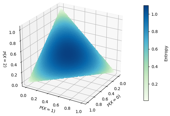
Figure 1: Entropy for 50K randomly sampled probability distributions of a discrete variable with 3 states. Entropy is maximized for uniform distributions (centre), minimized for one-hot distributions (corners). Lower entropy of any distribution $a$ compared to any distribution $b$ is not a sufficient condition for fewer non-zero states in $a$ (there exist darker points on the edges than on the interior), but as the color gradient implies, minimizing entropy via local optimization of probability mass is sufficient for decreasing the number of non-zero states across optimization timesteps.

2 Discrete variable case

Consider a vector of non-negative reals, $z\in\mathcal{R}_{\geq 0}^{s}$, which represents the unnormalized probability mass of a discrete variable $X$ taking each of $s$ states. Then the normalized probabilities are $\mathcal{P}(X=i|z)=\frac{z_{i}}{\sum_{j}z_{j}}$ where $j\in[0,s)$ is left implicit for readability, and entropy is:

$$\mathcal{H}(z)\triangleq-\sum_{i}\frac{z_{i}}{\sum_{j}z_{j}}\log\frac{z_{i}}{\sum_{j}z_{j}}.$$ (1)

Corollary 2.1.

Gradient of entropy with respect to each probability mass.

$$\frac{d\mathcal{H}(z)}{dz_{k}} =\frac{d}{dz_{k}}\Bigg{(}-\frac{z_{k}}{\sum_{j}z_{j}}\log\frac{z_{k}}{\sum_{j}z_{j}}-\sum_{i\neq k}\frac{z_{i}}{\sum_{j}z_{j}}\log\frac{z_{i}}{\sum_{j}z_{j}}\Bigg{)}$$ (2)

$$=\frac{-\sum_{i\neq k}z_{i}}{\big{(}\sum_{j}z_{j}\big{)}^{2}}+\frac{-\sum_{i\neq k}z_{i}}{\big{(}\sum_{j}z_{j}\big{)}^{2}}\log\frac{z_{k}}{\sum_{j}z_{j}}-\sum_{i\neq k}\bigg{(}\frac{-z_{i}}{\big{(}\sum_{j}z_{j}\big{)}^{2}}+\frac{-z_{i}}{\big{(}\sum_{j}z_{j}\big{)}^{2}}\log\frac{z_{i}}{\sum_{j}z_{j}}\bigg{)}$$ (3)

$$=\frac{-\sum_{i\neq k}z_{i}}{\big{(}\sum_{j}z_{j}\big{)}^{2}}\Bigg{(}1+\log\frac{z_{k}}{\sum_{j}z_{j}}\Bigg{)}-\sum_{i\neq k}\frac{-z_{i}}{\big{(}\sum_{j}z_{j}\big{)}^{2}}\bigg{(}1+\log\frac{z_{i}}{\sum_{j}z_{j}}\bigg{)}$$ (4)

$$=\frac{-\sum_{i\neq k}z_{i}}{\big{(}\sum_{j}z_{j}\big{)}^{2}}\Bigg{(}\log\frac{z_{k}}{\sum_{j}z_{j}}\Bigg{)}+\sum_{i\neq k}\frac{z_{i}}{\big{(}\sum_{j}z_{j}\big{)}^{2}}\bigg{(}\log\frac{z_{i}}{\sum_{j}z_{j}}\bigg{)}$$ (5)

$$=\frac{1}{\big{(}\sum_{j}z_{j}\big{)}^{2}}\sum_{i\neq k}z_{i}\log\frac{z_{i}}{z_{k}}$$ (6)

$$=\frac{1}{\big{(}\sum_{j}z_{j}\big{)}^{2}}\sum_{i}z_{i}\log\frac{z_{i}}{z_{k}}$$ (7)

$$\bigg{[}=\frac{1}{\big{(}\sum_{j}z_{j}\big{)}^{2}}\sum_{i}z_{i}\bigg{(}\log\frac{z_{i}}{\sum_{j}z_{j}}-\log\frac{z_{k}}{\sum_{j}z_{j}}\bigg{)}$$ (8)

$$=\frac{1}{\sum_{j}z_{j}}\sum_{i}\mathcal{P}(X=i|z)\log\frac{\mathcal{P}(X=i|z)}{\mathcal{P}(X=k)}\bigg{]}.$$ (9)

Consider taking one gradient step of minimizing entropy $\mathcal{H}$ with respect to masses $z$, $\tilde{z}_{k}=\max(z_{k}-\eta\frac{d\mathcal{H}}{dz_{k}},0)$, where $\eta$ is a learning rate hyperparameter. The following results follow directly from the equation for $\frac{d\mathcal{H}}{dz}$ in eq. 7.

Corollary 2.2.

State with the smallest non-zero mass always decreases in mass, and state with the largest mass always increases in mass. Follows directly from corollary 2.1; the smallest non-zero mass (and any zero masses) has a positive gradient, and the largest mass has a negative gradient.

Corollary 2.3.

Condition for whether a state’s mass decreases or increases. A necessary and sufficient condition for the gradient to be positive (i.e. the mass should be decreased to decrease entropy) is the log mass of the state being less than the weighted average of all log masses:

$$\frac{d\mathcal{H}}{dz_{k}}>0\longleftrightarrow\log z_{k}<\sum_{i}\frac{z_{i}}{\sum_{j}z_{j}}\log z_{i},$$ (10)

and vice versa for negative gradient or increase in mass.

Corollary 2.4.

Mass order is preserved and gaps are widened. For all $k,k^{\prime}:z_{k}<z_{k^{\prime}}$, the decrease in mass $z_{k}$ is larger than the decrease in mass $z_{k^{\prime}}$, meaning gradients decrease monotonically going from the smallest to largest non-zero masses:

$$\eta\frac{d\mathcal{H}}{dz_{k}}>\eta\frac{d\mathcal{H}}{dz_{k^{\prime}}}\longleftrightarrow\sum_{i}z_{i}\log z_{k}<\sum_{i}z_{i}\log z_{k^{\prime}}\longleftrightarrow\top.$$ (11)

Corollary 2.5.

Unless the masses start as uniform, they are never uniform during entropy minimization. Follows directly from corollary 2.4.

Corollary 2.6.

Zero masses stick to zero. Equation 10 is always true if $z_{k}=0$, but $z$ is defined on the non-negative reals, so states with probability 0 stay at probability 0.

Corollary 2.7.

Sum of gradients of masses is positive. From lemma A.1, for any non-uniform $a\in\mathcal{R}_{\geq 0}^{s}$, $\sum_{j}\sum_{i}a_{i}\log\frac{a_{i}}{a_{j}}>0$. Therefore $\sum_{k}\frac{d\mathcal{H}(z)}{dz_{k}}=\frac{1}{\big{(}\sum_{j}z_{j}\big{)}^{2}}\sum_{k}\sum_{i}z_{i}\log\frac{z_{i}}{z_{k}}$ $>0$. This implies average mass gradient is positive, $\frac{1}{s}\sum_{k}\frac{d\mathcal{H}(z)}{dz_{k}}>0$, and total mass is guaranteed to decrease in any iteration where no gradients are clipped to maintain non-negative masses, $\sum_{j}\tilde{z}_{j}<\sum_{j}z_{j}$.

Corollary 2.8.

Probability order is preserved. This follows from corollary 2.4, since mass order is preserved and the new probabilities are the new masses divided by a value that is constant across all states.

Corollary 2.9.

Change in probability for each state. Consider the case where the smallest non-zero mass state in $z$ still has positive mass in $\tilde{z}$ (otherwise, we know the number of non-zero probability states decreases). Since this state maintains positive mass, all states with greater mass in $z$ also maintain positive mass, by corollary 2.4, so none of their gradients are clipped in the optimization step. Then for any non-zero mass state in $z$ with index $i$, its increase in probability is given by:

$$\frac{z_{i}-\frac{\eta}{(\sum_{l}z_{l})^{2}}\sum_{k}z_{k}\log\frac{z_{k}}{z_{i}}}{\sum_{j}z_{j}-\frac{\eta}{(\sum_{l}z_{l})^{2}}\sum_{k}z_{k}\log\frac{z_{k}}{z_{j}}}-\frac{z_{i}}{\sum_{j}z_{j}}$$ (12)

$$= \frac{\eta}{c}\bigg{[}\overbrace{z_{i}\sum_{j}\frac{1}{(\sum_{l}z_{l})^{2}}\sum_{k}z_{k}\log\frac{z_{k}}{z_{j}}}^{\text{mass for $i$ $\times$ mass gradients for all $j$}}-\overbrace{(\sum_{j}z_{j})\frac{1}{(\sum_{l}z_{l})^{2}}\sum_{k}z_{k}\log\frac{z_{k}}{z_{i}}}^{\text{mass for all $j$ $\times$ mass gradient for $i$ }}\bigg{]},$$ (13)

where $c=(\sum_{j}z_{j})(\sum_{j}z_{j}-\frac{\eta}{(\sum_{l}z_{l})^{2}}\sum_{k}z_{k}\log\frac{z_{k}}{z_{j}})>0$ is the same for all $i$.

Corollary 2.10.

State with the smallest non-zero probability always decreases in probability, and state with the largest probability always increases in probability. From corollary 2.9, the increase in probability for state $i$ is $\frac{\eta}{c}>0$ multiplied by:

$$\bigg{(}z_{i}\sum_{j}\frac{1}{(\sum_{l}z_{l})^{2}}\sum_{k}z_{k}\log\frac{z_{k}}{z_{j}}\bigg{)}-\bigg{(}(\sum_{j}z_{j})\frac{1}{(\sum_{l}z_{l})^{2}}\sum_{k}z_{k}\log\frac{z_{k}}{z_{i}}\bigg{)}$$ (14)

$$=s\hskip 2.5ptz_{i}\hskip 2.5pt\gamma-s\hskip 2.5pt\mu\hskip 2.5pt\frac{d\mathcal{H}(z)}{dz_{i}},$$ (15)

where $\gamma=\frac{1}{s}\sum_{k}\frac{d\mathcal{H}(z)}{dz_{k}}>0$ (corollary 2.7) and $\mu=\frac{1}{s}\sum_{k}z_{k}>0$ and denote average gradient and mass. For the smallest non-zero mass, $0<z_{i}<\mu$ and $0<\frac{d\mathcal{H}(z)}{dz_{i}}>\gamma$, and for the largest mass, $z_{i}>\mu>0$ and $0>\frac{d\mathcal{H}(z)}{dz_{i}}<\gamma$.

Corollary 2.11.

Uniform distribution uniquely maximises entropy, non-unique one-hot distributions minimize it. These are the cases where $\forall k:\tilde{z}_{k}-z_{k}=0$: either when the masses are all equal so $\frac{d\mathcal{H}}{dz}=\bar{0}$, or there is only one non-zero mass, in which case the non-zero mass has gradient 0 and the zero masses have gradient $\infty$, staying clamped at 0. These critical points can also be found using Lagrangian constrained optimization (a tutorial is given in Morais (2018)).

Theorem 2.12.

The decrease in the probability of the smallest non-zero mass is lower bounded by a value that is $>0$ and increases with time, so applying gradient descent decreases the number of non-zero probability states in a finite number of iterations. More concretely, let $z^{t}$ be the vector of non-uniform masses at timestep $t$ and let the number of non-zero states in it be $c^{t}\triangleq\sum_{i=0}^{s-1}\mathbbm{1}_{z^{t}_{i}>0}$. For each timestep $t\in\mathcal{N}$ where $c^{t}>1$, there exists finite $\tilde{t}$ where $c^{\tilde{t}}<c^{t}$, and therefore there exists finite $t^{*}$ such that $c^{t^{*}}=1$.

We prove that at any time step $t$, the number of non-zero masses decreases given a finite number of subsequent optimization steps. In timestep $t$, assume the case where the state with smallest non-zero mass does not reach 0 mass in $t+1$, otherwise the statement is trivially satisfied. This implies none of the states with greater or equal mass decrease to 0 (corollary 2.4). Let the smallest non-zero mass state have index $i$. From corollary 2.9, the decrease in its probability is given by:

$$\hskip 2.5pt\frac{\eta}{c}\hskip 2.5pt\bigg{(}\bigg{(}(\sum_{j}z^{t}_{j})\frac{1}{(\sum_{l}z^{t}_{l})^{2}}\sum_{k}z^{t}_{k}\log\frac{z^{t}_{k}}{z^{t}_{i}}\bigg{)}-\bigg{(}z^{t}_{i}\sum_{j}\frac{1}{(\sum_{l}z^{t}_{l})^{2}}\sum_{k}z^{t}_{k}\log\frac{z^{t}_{k}}{z^{t}_{j}}\bigg{)}\bigg{)}$$ (16)

$$>\frac{\eta}{c}\hskip 2.5pt\bigg{(}\bigg{(}(\sum_{j}z^{t}_{j})\frac{1}{(\sum_{l}z^{t}_{l})^{2}}\sum_{k}z^{t}_{k}\log\frac{z^{t}_{k}}{z^{t}_{i}}\bigg{)}-\bigg{(}z^{t}_{i}\sum_{j}\frac{1}{(\sum_{l}z^{t}_{l})^{2}}\sum_{k}z^{t}_{k}\log\overbrace{\frac{z^{t}_{k}}{z^{t}_{i}}}^{\text{replaced $z^{t}_{j}$}}\bigg{)}\bigg{)}$$ (17)

$$=\frac{\eta}{c}\hskip 2.5pt\bigg{(}(\sum_{j}z^{t}_{j})-s\hskip 2.5ptz^{t}_{i}\bigg{)}\bigg{(}\frac{1}{(\sum_{l}z^{t}_{l})^{2}}\sum_{k}z^{t}_{k}\log\frac{z^{t}_{k}}{z^{t}_{i}}\bigg{)}$$ (18)

$$=\frac{\eta}{c}\hskip 2.5pt\bigg{(}1-s\hskip 2.5pt\mathcal{P}(X=i|z^{t})\bigg{)}\bigg{(}\sum_{k}\frac{z^{t}_{k}}{\sum_{l}z^{t}_{l}}\log\frac{z^{t}_{k}}{z^{t}_{i}}\bigg{)}$$ (19)

$$>0,$$ (20)

using that $\frac{\eta}{c}>0$, gradient of smallest non-zero mass is positive (corollary 2.2), and $\mathcal{P}(X=i|z^{t})<\frac{1}{s}$, since $i$ is the smallest element and we assumed the masses are non-uniform (which is reasonable; corollary 2.5). Therefore the decrease in the probability of the smallest element is lower bounded by a positive value. Now we show that this lower bound on $i$’s decrease increases with time (that is, if one assumes the worst case of minimal decrease, it speeds up). Let $z^{t}_{m}$ be the second value in the ascending-sorted vector of non-zero masses in $z^{t}$. From the lower bound in eq. 19:

$$\hskip 2.5pt\frac{\eta}{c}\bigg{(}1-s\hskip 2.5pt\mathcal{P}(X=i|z^{t})\bigg{)}\bigg{(}\sum_{k}\frac{z^{t}_{k}}{\sum_{l}z^{t}_{l}}\log\frac{z^{t}_{k}}{z^{t}_{i}}\bigg{)}$$ (21)

$$=\frac{\eta}{c}\bigg{(}1-s\hskip 2.5pt\mathcal{P}(X=i|z^{t})\bigg{)}\bigg{(}\sum_{k\neq i}\frac{z^{t}_{k}}{\sum_{l}z^{t}_{l}}\log\frac{z^{t}_{k}}{z^{t}_{i}}\bigg{)}$$ (22)

$$\geq\frac{\eta}{c}\bigg{(}1-s\hskip 2.5pt\mathcal{P}(X=i|z^{t})\bigg{)}\bigg{(}\sum_{k\neq i}\frac{z^{t}_{k}}{\sum_{l}z^{t}_{l}}\log\overbrace{\frac{z^{t}_{m}}{z^{t}_{i}}}^{\text{replaced $z^{t}_{k}$}}\bigg{)}$$ (23)

$$=\frac{\eta}{c}(1-s\hskip 2.5pt\mathcal{P}(X=i|z^{t}))(1-\mathcal{P}(X=i|z^{t}))\log\frac{z^{t}_{m}}{z^{t}_{i}}.$$ (24)

Each of the 4 multiplicative factors in eq. 24 is positive and increases with time in any window of timesteps where no mass drops to 0; otherwise, we are done. The first 3 trivially so: $\eta$ is constant, $c$ is the product of old and new total masses and total masses decrease with time (corollary 2.7), $s$ is constant, $\mathcal{P}(X=i|z^{t})$ or the probability of the state with smallest mass decreases with time until it becomes 0 (corollaries 2.10 and 2.8). Now we show that the last term, the ratio between the second and first values in the sorted vector of non-zero masses, $z^{t}_{m}$ and $z^{t}_{i}$, increases with time.

$$\frac{z^{t}_{m}-\eta\frac{d\mathcal{H}(z^{t})}{dz^{t}_{m}}}{z^{t}_{i}-\eta\frac{d\mathcal{H}(z^{t})}{dz^{t}_{i}}} >\frac{z^{t}_{m}}{z^{t}_{i}}$$ (25)

$$\longleftrightarrow-z^{t}_{i}\hskip 2.5pt\eta\frac{d\mathcal{H}(z^{t})}{dz^{t}_{m}} >-z^{t}_{m}\hskip 2.5pt\eta\frac{d\mathcal{H}(z^{t})}{dz^{t}_{i}}$$ (26)

$$\longleftrightarrow z^{t}_{i}\hskip 2.5pt\frac{d\mathcal{H}(z^{t})}{dz^{t}_{m}} <z^{t}_{m}\hskip 2.5pt\frac{d\mathcal{H}(z^{t})}{dz^{t}_{i}}$$ (27)

$$\longleftrightarrow z^{t}_{i}\hskip 2.5pt\sum_{j}z^{t}_{j}\log\frac{z^{t}_{j}}{z^{t}_{m}} <z^{t}_{m}\hskip 2.5pt\sum_{j}z^{t}_{j}\log\frac{z^{t}_{j}}{z^{t}_{i}}$$ (28)

$$\longleftrightarrow z^{t}_{i}\hskip 2.5pt\bigg{(}(\sum_{j}z^{t}_{j}\log z^{t}_{j})-(\sum_{j}z^{t}_{j})\log z^{t}_{m}\bigg{)} <z^{t}_{m}\hskip 2.5pt\bigg{(}(\sum_{j}z^{t}_{j}\log z^{t}_{j})-(\sum_{j}z^{t}_{j})\log z^{t}_{i}\bigg{)}$$ (29)

$$\longleftrightarrow(\sum_{j}z^{t}_{j})(z^{t}_{m}\log z^{t}_{i}-z^{t}_{i}\log z^{t}_{m}) <(z^{t}_{m}-z^{t}_{i})(\sum_{j}z^{t}_{j}\log z^{t}_{j})$$ (30)

$$\longleftrightarrow\frac{z^{t}_{m}\log z^{t}_{i}-z^{t}_{i}\log z^{t}_{m}}{z^{t}_{m}-z^{t}_{i}} <\frac{\sum_{j}z^{t}_{j}\log z^{t}_{j}}{\sum_{j}z^{t}_{j}}$$ (31)

$$\longleftarrow\frac{z^{t}_{m}\log z^{t}_{i}-z^{t}_{i}\log\overbrace{z^{t}_{i}}^{\text{replaced }z^{t}_{m}}}{z^{t}_{m}-z^{t}_{i}} <\frac{\sum_{j}z^{t}_{j}\log z^{t}_{j}}{\sum_{j}z^{t}_{j}}$$ (32)

$$\longleftrightarrow\frac{(z^{t}_{m}-z^{t}_{i})\log z^{t}_{i}}{z^{t}_{m}-z^{t}_{i}} <\frac{\sum_{j}z^{t}_{j}\log z^{t}_{j}}{\sum_{j}z^{t}_{j}}$$ (33)

$$\longleftrightarrow \top.$$ (34)

$\square$.

2.1 Expected cardinality of sampled sets

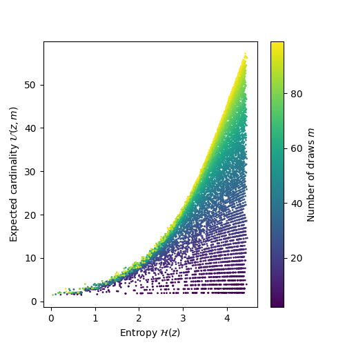
Figure 2: Entropy plotted against expected number of unique states drawn, for 10K samples of masses $z$ with random length $s=|z|\in[2,100]$ and draws $m\in[2,100]$. The upper bound on expected number of unique draws goes up with $m$ because it is not possible to draw more than $m$ unique states if $m$ is the number of draws.

Now let us consider a different quantity, the expected cardinality or number of unique states obtained with $m$ draws of $X$, $\mathcal{U}(z,m)$. Let $I_{i}$ be 1 if we draw at least 1 sample from the $i^{th}$ state of $X$, and 0 if we draw none. Then:

$$\mathcal{U}(z,m) \triangleq\mathbb{E}\big{[}\sum_{i}I_{i}\big{]}=\sum_{i}\mathbb{E}\big{[}I_{i}\big{]}\qquad\text{(linearity of expectation)}$$ (35)

$$=\sum_{i}0P(I_{i}=0|z)+1P(I_{i}=1|z)$$ (36)

$$=\sum_{i}1-\bigg{(}1-\frac{z_{i}}{\sum_{j}z_{j}}\bigg{)}^{m},$$ (37)

which is strictly less than the standard cardinality of the set of possible states, $\sum_{i=0}^{s-1}\mathbbm{1}_{z_{i}>0}$. The gradient with respect to each mass is:

$$\frac{d\mathcal{U}(z,m)}{dz_{k}}=\frac{d}{dz_{k}}\bigg{(}1-\bigg{(}1-\frac{z_{k}}{\sum_{j}z_{j}}\bigg{)}^{m}\bigg{)}+\sum_{i\neq k}\frac{d}{dz_{k}}\bigg{(}1-\bigg{(}1-\frac{z_{i}}{\sum_{j}z_{j}}\bigg{)}^{m}\bigg{)}$$ (38)

$$=-m\bigg{(}1-\frac{z_{k}}{\sum_{j}z_{j}}\bigg{)}^{m-1}\frac{d}{dz_{k}}\bigg{(}-\frac{z_{k}}{\sum_{j}z_{j}}\bigg{)}+\sum_{i\neq k}-m\bigg{(}1-\frac{z_{i}}{\sum_{j}z_{j}}\bigg{)}^{m-1}\frac{d}{dz_{k}}\bigg{(}-\frac{z_{i}}{\sum_{j}z_{j}}\bigg{)}$$ (39)

$$=-m\bigg{(}1-\frac{z_{k}}{\sum_{j}z_{j}}\bigg{)}^{m-1}\frac{z_{k}-\sum_{i}z_{i}}{\big{(}\sum_{j}z_{j}\big{)}^{2}}+\sum_{i\neq k}-m\bigg{(}1-\frac{z_{i}}{\sum_{j}z_{j}}\bigg{)}^{m-1}\frac{z_{i}}{\big{(}\sum_{j}z_{j}\big{)}^{2}}$$ (40)

$$=\frac{m}{\big{(}\sum_{j}z_{j}\big{)}^{2}}\sum_{i}z_{i}\bigg{(}\bigg{(}1-\frac{z_{k}}{\sum_{j}z_{j}}\bigg{)}^{m-1}-\bigg{(}1-\frac{z_{i}}{\sum_{j}z_{j}}\bigg{)}^{m-1}\bigg{)}.$$ (41)

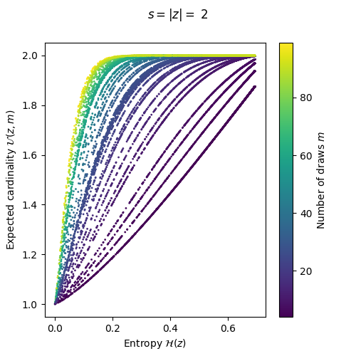
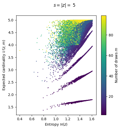
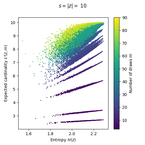
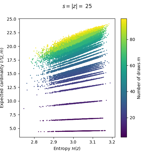
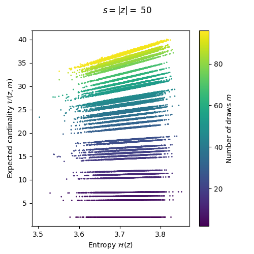
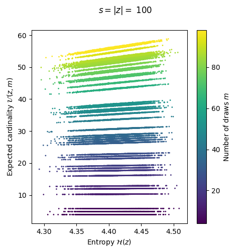
Figure 3: Partial breakdown of fig. 2 grouped by $s=|z|$, the length of the mass vector or maximum number of possible states. Reducing entropy is not a sufficient condition for reducing expected cardinality in general, given fixed $s$ and $m$, but we show that local optimization via gradient descent on entropy with respect to probability masses is sufficient.

Entropy $\mathcal{H}$ and expected number of unique state draws $\mathcal{U}$ are related. This is suggested by the similar forms of their gradients (eqs. 8 and 41), and also empirically (fig. 2). A breakdown of fig. 2 into different fixed lengths of $z$ is in fig. 3. To understand the relationship between the two quantities, note that one intuitively expects higher entropy distributions to have higher expected number of unique draws, given some fixed number of draws. For example, for probability distributions [0.5, 0.5] and [0.9, 0.1], observing both states is more likely sooner with the former. Reducing entropy makes the distribution more skewed (section 2), therefore sampling more unfair, which reduces the expected number of seen states for any number of draws.

Theorem 2.13.

Gradient descent on entropy $\mathcal{H}(z)$ decreases the expected number of unique states in $m$ draws, $\mathcal{U}(z,m)$, for any fixed $m>1$.

Without loss of generality since $\mathcal{H}(z)$ and $\mathcal{U}(z,m)$ are invariant to order of $z$, assume $z$ is sorted in ascending order, and therefore also $\tilde{z}$ (corollary 2.4). Define $p_{i}\triangleq\frac{z_{i}}{\sum_{j}z_{j}}$, $q_{i}\triangleq 1-p_{i}$ and similarly $\tilde{p}_{i}\triangleq\frac{\tilde{z}_{i}}{\sum_{j}\tilde{z}_{j}}$ and $\tilde{q}\triangleq 1-\tilde{p}_{i}$.

When $m=1$: $\mathcal{U}(z,1)-\mathcal{U}(\tilde{z},1)=0\longleftrightarrow\sum_{i}\tilde{q}_{i}-q_{i}=\sum_{i}(1-\tilde{p}_{i})-(1-p_{i})=0\leftrightarrow\top$. When $m>1$, $\mathcal{U}(z,m)$ decreases during gradient descent on $\mathcal{H}(z)$ iff:

$$\mathcal{U}(z,m)-\mathcal{U}(\tilde{z},m) >0$$ (42)

$$\longleftrightarrow\sum_{i}1-q_{i}^{m}-(1-\tilde{q}_{i}^{m}) >0$$ (43)

$$\longleftrightarrow\sum_{i}\tilde{q}_{i}^{m} >\sum_{i}q_{i}^{m}$$ (44)

$$\longleftarrow\sum_{i}\tilde{q}_{i}^{m}>\sum_{i}q_{i}\hskip 2.5pt\tilde{q}_{i}^{m-1} \land\sum_{i}q_{i}\hskip 2.5pt\tilde{q}_{i}^{m-1}>\sum_{i}q_{i}^{m}.$$ (45)

Now we prove the truth of both conditions in eq. 45. For the first condition in eq. 45:

$$\sum_{i}\tilde{q}_{i}^{m} >\sum_{i}q_{i}\hskip 2.5pt\tilde{q}_{i}^{m-1}$$ (46)

$$\longleftrightarrow\sum_{i}\tilde{q}_{i}\hskip 2.5pt\tilde{q}_{i}^{m-1} >\sum_{i}q_{i}\hskip 2.5pt\tilde{q}_{i}^{m-1}$$ (47)

$$\longleftrightarrow\sum_{i}\tilde{q}_{i}^{m-1}\hskip 2.5pt(\tilde{q}_{i}-q_{i}) >0.$$ (48)

Since masses $z$ and $\tilde{z}$ are sorted in ascending order, so are probabilities $p$ and $\tilde{p}$. So $q$ and $\tilde{q}$ are both sorted in decreasing order. The vector of changes in state probabilities $\tilde{p}-p$ consists of a sequence of non-positive values followed by a sequence of positive values, and sums to 0. Then $\tilde{q}-q=(1-\tilde{p})-(1-p)=-(\tilde{p}-p)$ consists of a sequence of non-negative values followed by a sequence of negative values, and also sums to 0. Since $\tilde{q}$ is soted in decreasing order, so is $\tilde{q}^{m-1}$. Therefore by lemma A.2, eq. 48 is true.

For the second condition in eq. 45. Let $\mu\triangleq\frac{1}{s}\sum_{i}\tilde{q}_{i}^{m-1}-q_{i}^{m-1}$:

$$\sum_{i}q_{i}\hskip 2.5pt\tilde{q}_{i}^{m-1} >\sum_{i}q_{i}^{m}$$ (49)

$$\longleftrightarrow\sum_{i}q_{i}\hskip 2.5pt\tilde{q}_{i}^{m-1} >\sum_{i}q_{i}\hskip 2.5ptq_{i}^{m-1}$$ (50)

$$\longleftrightarrow\sum_{i}q_{i}(\tilde{q}_{i}^{m-1}-q_{i}^{m-1}) >0$$ (51)

$$\longleftrightarrow\bigg{(}\sum_{i}q_{i}(\tilde{q}_{i}^{m-1}-q_{i}^{m-1}-\mu)\bigg{)}+\mu\sum_{i}q_{i} >0.$$ (52)

The first term in eq. 52 is positive by lemma A.2. Second term is $\geq 0$ because $\sum_{i}q_{i}$ is positive and $\mu$ is positive or zero (proof by induction, i.e. assuming eq. 42 and therefore eq. 44 for $m-1$). $\square$.

3 Continuous variable case

In continuous spaces, a standard distribution-invariant measure for size is covering number, which is the cardinality of the smallest set of partitions that cover the space, for a given distance metric $\rho$ and upper bound on partition width $\epsilon$.

Definition 3.1 (Van Der Vaart et al. (1996)).

For a metric space $S,\rho$ and $T\subset S$, $\hat{T}\subset S$ is an $\epsilon$-cover of $T$, if $\forall t\in T$, $\exists\hat{t}\in\hat{T}$ such that $\rho(t,\hat{t})\leq\epsilon$. The $\epsilon$-covering number of $T$ is

$$\mathcal{N}(\epsilon,T,\rho)=\min\{|\hat{T}|\,:\hat{T}\mbox{ is an }\epsilon-\mbox{cover of }T\}.$$

We provide two arguments for the link between minimizing entropy and covering number for probability distributions defined on continuous variables. First, differential entropy is the limiting case of discrete entropy: $\int_{x}\mathcal{P}(x)\log\mathcal{P}(x)\hskip 2.5ptdx=\lim_{s\rightarrow\infty}\sum_{i=0}^{s-1}(\mathcal{P}(x_{i})\log\mathcal{P}(x_{i}))\triangle x$, and the arguments in section 2 hold given any discretization of the continuous support of $\mathcal{X}$ into finite partitions.

Secondly, the relationship is clear to see for specific cases of continuous probability distributions where entropy can be analytically computed. In the case of the uniform distribution defined on the continuous range of scalars $[a,b]$, entropy is $\ln(b-a)$, and since $\ln$ is monotonically increasing, decreasing entropy corresponds to monotonically decreasing the range, which reduces the $\epsilon$-covering number in a finite number of timesteps assuming a positive lower bound for the reduction in range in each optimization timestep. In the case of the independent multivariate Gaussian distribution on variable $X\in\mathcal{R}^{k}$ (i.e. the covariance matrix is diagonal and components are independent), entropy is given by $\frac{1}{2}\sum_{i=0}^{k-1}\ln(2\pi e\operatorname{Var}[X_{i}])$ (Norwich, 1993), so gradient descent on entropy with respect to the variance of each component implies a monotonic decrease in the latter. The smaller the variance of a Gaussian, the sharper it becomes, and the fewer the number of covering partitions with non-negligible probability mass, given any partitioning of the unbounded support of the distribution.

In practice, minimizing entropy of a data representation $X\in\mathcal{R}^{k}$ (which is suggested by information bottleneck, Ahuja et al. (2021); Tishby et al. (2000)) can be implemented as minimizing the empirical variance of each of the $k$ components in the representation vector. The rationale is that the multivariate normal distribution is the maximum entropy distribution for a given covariance, the entropy of the multivariate normal distribution is upper bounded by entropy of the independent variable case of the multivariate normal distribution (Kirsch et al., 2020), and the entropy of the latter is a sum of logs of the variance of each component variable, as we have seen. Gradient descent on the empirical variance with respect to the representation of each sample corresponds to moving the representations closer to the mean, as $\frac{d\sigma^{2}}{dx_{k}}=\frac{d\frac{1}{n}\sum_{i=0}^{n-1}(x_{i}-\bar{x})^{2}}{dx_{k}}=\frac{2}{n}(x_{k}-\bar{x})$, which contracts the space.

Acknowledgements.

We are grateful for discussions with Razvan Pascanu, Aristide Baratin, and Yoshua Bengio. The first author is supported by funding from IVADO.

Appendix A Lemmas

Lemma A.1.

For any $a\in\mathcal{R}_{\geq 0}^{s}$ of non-identical values, $\sum_{j}\sum_{i}a_{i}\log\frac{a_{i}}{a_{j}}>0$.

We prove this by induction. Without loss of generality since order is immaterial for the sums in lemma A.1, assume $a$ is sorted in ascending order. The base case, considering only the first 2 elements of $a$, $a_{1}\geq a_{0}$, is given by:

$$a_{0}\log\frac{a_{0}}{a_{1}}+a_{1}\log\frac{a_{1}}{a_{0}}+a_{0}\log\frac{a_{0}}{a_{0}}+a_{1}\log\frac{a_{1}}{a_{1}} \geq 0$$ (53)

$$\longleftrightarrow a_{0}\log\frac{a_{0}}{a_{1}}+a_{1}\log\frac{a_{1}}{a_{0}} \geq 0$$ (54)

$$\longleftrightarrow a_{1}\log\frac{a_{1}}{a_{0}} \geq-a_{0}\log\frac{a_{0}}{a_{1}}$$ (55)

$$\longleftrightarrow\frac{-a_{1}}{a_{0}} \leq\frac{\log\frac{a_{0}}{a_{1}}}{\log\frac{a_{1}}{a_{0}}}$$ (56)

$$\longleftrightarrow\frac{a_{1}}{a_{0}} \geq\frac{\log\frac{a_{1}}{a_{0}}}{\log\frac{a_{1}}{a_{0}}}$$ (57)

$$\longleftrightarrow \top,$$ (58)

where the inequalities are strict iff $a_{1}>a_{0}$. The inductive case, considering the first $k$ elements and assuming $\sum_{j=0}^{k-1}\sum_{i=0}^{k-1}a_{i}\log\frac{a_{i}}{a_{j}}\geq 0$ holds for the first $k-1$ elements:

$$\sum_{j=0}^{k}\sum_{i=0}^{k}a_{i}\log\frac{a_{i}}{a_{j}} \geq 0$$ (59)

$$\longleftrightarrow a_{k}\log\frac{a_{k}}{a_{k}}+\bigg{(}\sum_{i=0}^{k-1}a_{i}\log\frac{a_{i}}{a_{k}}+a_{k}\log\frac{a_{k}}{a_{i}}\bigg{)}+\bigg{(}\sum_{j=0}^{k-1}\sum_{i=0}^{k-1}a_{i}\log\frac{a_{i}}{a_{j}}\bigg{)} \geq 0$$ (60)

$$\longleftarrow\sum_{i=0}^{k-1}a_{i}\log\frac{a_{i}}{a_{k}}+a_{k}\log\frac{a_{k}}{a_{i}} \geq 0$$ (61)

$$\longleftrightarrow\sum_{i=0}^{k-1}a_{i}\log a_{i}+a_{k}\log a_{k}-a_{i}\log a_{k}-a_{k}\log a_{i} \geq 0$$ (62)

$$\longleftrightarrow\sum_{i=0}^{k-1}(a_{k}-a_{i})\log a_{k}-(a_{k}-a_{i})\log a_{i} \geq 0$$ (63)

$$\longleftrightarrow\sum_{i=0}^{k-1}(a_{k}-a_{i})(\log a_{k}-\log a_{i}) \geq 0$$ (64)

$$\longleftrightarrow \top,$$ (65)

where the inequalities are strict if $a_{0\dots k}$ is not a vector of identical values. $\square$.

Lemma A.2.

Let $w\in\mathcal{R}_{\geq 0}^{s}$ be any non-uniform vector of non-negative reals sorted in descending order, so $\forall i:w_{i}\geq w_{i+1}$. Let $x\in\mathcal{R}^{s}$ be any non-uniform vector of reals that sums to 0 and consists of a contiguous sequence of non-negative values followed by a contiguous sequence of negative values, so $\sum_{i}x_{i}=0$ and $\exists l\in[1,|x|-1]$ such that $\forall i\in[0,l):x_{i}\geq 0$, $\forall i\in[l,|x|):x_{i}<0$. Then dot product $w^{\intercal}x>0$ is positive.

Let $A=[0,l)$ be the indices of all non-negative elements in $x$ and $B=[l,|x|)$ be the indices of all negative elements in $x$.

$$\sum_{i}w_{i}\hskip 2.5ptx_{i} >0$$ (66)

$$\longleftrightarrow\bigg{(}\sum_{a\in A}w_{a}\hskip 2.5ptx_{a}\bigg{)}+\bigg{(}\sum_{b\in B}w_{b}\hskip 2.5ptx_{b}\bigg{)} >0$$ (67)

$$\longleftrightarrow\overbrace{\bigg{(}\sum_{a\in A}x_{a}\bigg{)}}^{g_{A}>0}\overbrace{\bigg{(}\frac{\sum_{a\in A}w_{a}\hskip 2.5ptx_{a}}{\sum_{a\in A}x_{a}}\bigg{)}}^{f_{A}>0}+\overbrace{\bigg{(}\sum_{b\in B}x_{b}\bigg{)}}^{g_{B}<0}\overbrace{\bigg{(}\frac{\sum_{b\in B}w_{b}\hskip 2.5ptx_{B}}{\sum_{b\in B}x_{b}}\bigg{)}}^{f_{B}>0} >0$$ (68)

$$\longleftrightarrow f_{A}\hskip 2.5ptg_{A} >-f_{B}\hskip 2.5ptg_{B}$$ (69)

$$\longleftrightarrow\frac{f_{A}}{f_{B}} >-\frac{g_{B}}{g_{A}}$$ (70)

$$\longleftrightarrow\frac{f_{A}}{f_{B}} >\frac{g_{A}}{g_{A}}=1$$ (71)

$$\longleftrightarrow\top,$$ (72)

because $g_{A}+g_{B}=0$ and $f_{A}>f_{B}$. $\square$.

References

- Ahuja et al. (2021) Kartik Ahuja, Ethan Caballero, Dinghuai Zhang, Yoshua Bengio, Ioannis Mitliagkas, and Irina Rish. Invariance principle meets information bottleneck for out-of-distribution generalization. arXiv preprint arXiv:2106.06607, 2021.
- Bassily et al. (2018) Raef Bassily, Shay Moran, Ido Nachum, Jonathan Shafer, and Amir Yehudayoff. Learners that use little information. In Algorithmic Learning Theory, pages 25–55. PMLR, 2018.
- Goyal and Bengio (2020) Anirudh Goyal and Yoshua Bengio. Inductive biases for deep learning of higher-level cognition. arXiv preprint arXiv:2011.15091, 2020.
- Ji et al. (2021) Xu Ji, Razvan Pascanu, Devon Hjelm, Balaji Lakshminarayanan, and Andrea Vedaldi. Test sample accuracy scales with training sample density in neural networks, 2021.
- Kirsch et al. (2020) Andreas Kirsch, Clare Lyle, and Yarin Gal. Unpacking information bottlenecks: Surrogate objectives for deep learning. 2020.
- Liu et al. (2021) Dianbo Liu, Alex Lamb, Kenji Kawaguchi, Anirudh Goyal, Chen Sun, Michael Curtis Mozer, and Yoshua Bengio. Discrete-valued neural communication. arXiv preprint arXiv:2107.02367, 2021.
- Mohri et al. (2018) Mehryar Mohri, Afshin Rostamizadeh, and Ameet Talwalkar. Foundations of machine learning. MIT press, 2018.
- Morais (2018) Mike Morais. Lecture 8: Information Theory and Maximum Entropy. http://pillowlab.princeton.edu/teaching/statneuro2018/slides/notes08_infotheory.pdf, 2018. [Online; accessed 13-November-2021].
- Norwich (1993) KH Norwich. The entropy of the normal distribution. Information, sensation, and perception, pages 81–87, 1993.
- Tack et al. (2020) Jihoon Tack, Sangwoo Mo, Jongheon Jeong, and Jinwoo Shin. Csi: Novelty detection via contrastive learning on distributionally shifted instances. arXiv preprint arXiv:2007.08176, 2020.
- Tishby et al. (2000) Naftali Tishby, Fernando C Pereira, and William Bialek. The information bottleneck method. arXiv preprint physics/0004057, 2000.
- Van Der Vaart et al. (1996) Aad W Van Der Vaart, Adrianus Willem van der Vaart, Aad van der Vaart, and Jon Wellner. Weak convergence and empirical processes: with applications to statistics. Springer Science & Business Media, 1996.
- Xu and Mannor (2012) Huan Xu and Shie Mannor. Robustness and generalization. Machine learning, 86(3):391–423, 2012.