Prototypical Model with Novel Information-theoretic Loss Function for Generalized Zero Shot Learning

Abstract

Generalized zero shot learning (GZSL) is still a technical challenge of deep learning as it has to recognize both source and target classes without data from target classes. To preserve the semantic relation between source and target classes when only trained with data from source classes, we address the quantification of the knowledge transfer and semantic relation from an information-theoretic viewpoint. To this end, we follow the prototypical model and format the variables of concern as a probability vector. Leveraging on the proposed probability vector representation, the information measurement such as mutual information and entropy, can be effectively evaluated with simple closed forms. We discuss the choice of common embedding space and distance function when using the prototypical model. Then We propose three information-theoretic loss functions for deterministic GZSL model: a mutual information loss to bridge seen data and target classes; an uncertainty-aware entropy constraint loss to prevent overfitting when using seen data to learn the embedding of target classes; a semantic preserving cross entropy loss to preserve the semantic relation when mapping the semantic representations to the common space. Simulation shows that, as a deterministic model, our proposed method obtains state of the art results on GZSL benchmark datasets. We achieve $21\%\thicksim 64\%$ improvements over the baseline model – deep calibration network (DCN) and for the first time demonstrate a deterministic model can perform as well as generative ones. Moreover, our proposed model is compatible with generative models. Simulation studies show that by incorporating with f-CLSWGAN, we obtain comparable results compared with advanced generative models.

1 Introduction

Deep convolutional neural networks gain remarkable successes in object recognition in recent years [8, 24, 42]. However, most successful deep neural networks are trained under supervised learning frameworks, which always require a large amount of annotated data for each class [13]. Inspired by human’s ability to recognize objects without having seen visual samples, recently, zero-shot learning (ZSL) gains a surge of interest and has been used in broad applications [32, 44, 25, 62, 53, 52, 11, 10, 61, 60, 54, 51].

ZSL offers an elegant way to extend classifiers from source categories, of which labeled images are available during training, to target categories, of which labeled images are not accessible. The goal of ZSL is to recognize objects of target classes by transferring knowledge from source classes through the relation in the semantic space, while generalized zero-shot learning (GZSL), a more general and challenging scenario of ZSL, tries to recognize objects from the joint set of both source and target classes.

Generally, methods for ZSL/GZSL can be categorized into two majors — deterministic and generative: Deterministic methods focus on carefully designed models and semantic relation preserving the knowledge from source classes to target classes, using only the seen data from source classes; Generative methods leverage on novel generative models to transfer the knowledge of the paired relation between the semantic representation and visual feature of source classes, in order to generate the data for target classes. With these generated data, although less reliable, generative methods always obtain superior performance than deterministic methods. Broad studies show that filling the performance gap between them is a challenge. Moreover, a common problem in both methods is how to trust the less reliable data, such as using seen data of source classes to train the embedding model of target classes or using the generated data of target classes to train the discriminative models, so that some uncertainty-aware strategies are required in such scenarios. These two problems are the primary concerns of this study.

Two technical problems as envisioned in deterministic ZSL/GZSL [10, 27]: (i) how to bridge source classes to target classes for knowledge transfer and (ii) how to make prediction on target classes without labeled training data. Toward the first problem, deterministic ZSL/GZSL methods typically embed the image features and the semantic representations into a predefined common embedding space (with properly defined distances) using a regression model. The choice of the embedding space and the design of regression model/neural network are essential to inherit the semantic relation meanwhile maintaining the discriminative ability. As for the second problem, we need to effectively bridge target classes to source classes by knowledge transfer such as retaining the structure of the semantic space, and prevent the overfitting in the seen data of source classes as they are blind to the semantic representations of target classes. The seminal work, deep calibration network (DCN) [27], introduces an entropy loss on target class which brings the semantic representations close to certain seen data of source classes. However, the entropy loss with a calibration parameter is not adequate to accurately control how much the target classes should learn from the seen data, which prevents the DCN from obtaining superior performance.

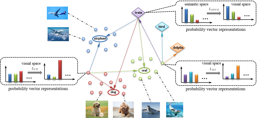
Figure 1: Illustration of probability vector representation for zero-shot learning. Circles and diamonds with text names denote the semantic representations of all classes, small dots denote seen data (or say visual features) of source classes, and unseen data of target classes are unavailable. The probability vector (PV) represents the probability that the data is assigned to different clustering centroids/prototypes, where the assignment is shown by the arrow. The training goal is intuitively illustrated by the change of bars in the PV representation.

Before the introduction of our major contributions, we address a uniform representation of the concerned variables by a soft assignment probability vector (PV), illustrated in Fig. 1. By regarding the semantic representation of either source or target classes as the clustering centroids, or say some reference points in the common space, the position of visual feature in this space can be formatted into a soft assignment PV under the prototypical model [43]: we characterize the position of visual feature indirectly by measuring its relation (assignment probability) to the reference points. We discuss the choice of projection model, the common space and the distance functions for the definition of the prototypical model based PV representation. Given such a uniform PV representation, we can evaluate the information measurements, such as mutual information, entropy, cross entropy with closed form expressions.

The major contributions: 1) we propose a mutual information loss to link the semantic representations of target classes to seen data of source classes. The mutual information consists of two parts: the conditional entropy encourages the seen data to attach to certain prototype/centroid of the target classes, while the entropy term preserving the semantic representations collapses to trivial solutions when projecting them to the visual space; 2) we propose an uncertainty-aware loss function which prevents overfitting when using seen data of source classes to train the embedding model of target classes. We define a regularized entropy, which allows us to compare/control the uncertainty of the seen data belonging to source and target classes; 3) we propose a semantic preserving loss function, which minimizes the cross entropy between the PV in original semantic space and in the visual space to preserve the semantic relation when learning the network that maps the semantic representations to the visual space.

We evaluate the performance of our proposed methods on broadly studied benchmark datasets. Simulation shows that, as a deterministic GZSL model, our proposed method obtains state of the art results, and outperforms significantly the recent deterministic models on all benchmark datasets. Our proposed model is compatible with generative models as well. We present additional loss functions to learn with generated data by considering their higher uncertainty than seen data. The experiments show that, by incorporating with generated data from f-CLSWGAN [55], we gain obvious improvement over the vanilla f-CLSWGAN model and for the first time demonstrate a deterministic model can perform as well as generative ones.

2 Related works

Deterministic models for GZSL. Deterministic models try to sufficiently utilize the knowledge of the semantic embedding of both source and target classes to conduct the inference on visual data. To this end, previous works typically embed visual samples and the semantic embedding to a common embedding space [15, 16, 61, 9], such as the visual space, the semantic embedding space or an intermediate space between semantic and visual domains. The choice of embedding space is critical for model performance. Previous works [41, 61] show that using visual space instead of semantic space or any other intermediate space as the common embedding space alleviates the negative effect of the hubness problem [36, 46, 26]. The choice of distance function in the common embedding space also plays an importance roll. In previous studies [49, 43, 37, 27], Euclidean distance, dot product similarity and cosine similarity are broadly applied.

The majority of the ZSL/GZSL methods tend to compensate the lack of visual representation of the unseen classes with the learning of a semantic preserving mapping. For instance, a fairly successful approach is based on a bi-linear compatibility function that associates visual representation and semantic features, such as ALE [1], DEVISE [15], SJE [3] and ESZSL [33]. A straightforward extension of the methods above is the exploration of a non-linear compatibility function between visual and semantic spaces, such as a ridge regression [41]. Furthermore, in [4], they introduce explicit regularization for semantic preserving but require an extra threshold for the similarity. In another seminal work [27], they introduce an entropy loss to allow the embedding network of target classes trained by seen data, and a calibration parameter is required to balance the training of source classes and target classes. In our work, we introduce a series of information-theoretic loss functions which enable the use of non-linear compatibility functions. Meanwhile, these functions allow us to translate several intuitive assumptions on the semantic relation to easy computing formulas. Moreover, we find that the conditional entropy in our mutual information loss is consistent with the entropy loss in [27], while the new marginal entropy term in our loss make additional effects to encourage cluster balancing.

Data-Generating Models for GZSL. Generative models possess the advantage of utilizing generated image features to remove the blindness as a result of inaccessible data of target classes during training. Variational Autoencoders (VAE) [23] and conditional VAE [45] based generative models are proposed with an aim to align the visual embedding with the semantic embedding [48, 39, 30, 21]. A VAE based algorithm can train stably, but it fails to capture the complex distribution [7], leading to unsatisfied results. Generative adversarial network (GAN) [17] has an advantage in generating more diverse data. The f-CLSWGAN [55] is the model including a variant of an improved WGAN [6] and a softmax classifier. f-CLSWGAN synthesizes visual features conditioned on semantic representations, offering a shortcut directly from a semantic descriptor to a class-conditional feature distribution. Despite strong performance, GAN always suffers from mode collapse issues and has a unstable training phase [5]. Fortunately, an improved deterministic model incorporated with a generative model leads to a more advanced performance[47]. In this work, we notice that the synthetic data from the generative model are generally less reliable than the seen data, so the uncertainty-aware entropy constraint loss is also applicable here. Thus, instead of constructing a complex generative model, we train the proposed model additionally with the generated data from an f-CLSWGAN, and obtain competitive results compared to recent advanced generative models.

3 Generalized Zero-shot learning

Following the notation in [27], we first present the definition of generalized zero-shot learning as follows: suppose we have the seen data $\mathcal{D}=\left\{(x^{(n)},y^{(n)})\right\}_{n=1}^{N}$, where $x^{(n)}\in\mathbb{R}^{P}$ is the feature of the $n$-th image in the visual space $\mathbb{R}^{P}$ and $y^{(n)}\in\mathcal{S}$ is the label from the source classes $\mathcal{S}=\{1,...,S\}$. In this study, we assume that the image feature $x$ (also named visual embedding) has already been extracted by a pretrained deep convolutional networks, such as ResNet [18]. Let $\mathcal{T}=\left\{S+1,...,S+T\right\}$ denote the target classes, where no seen data is available in the training phase. For each class $c\in\mathcal{S}\cup\mathcal{T}$, let $v_{c}\in\mathbb{R}^{Q}$ denote the semantic representation in the semantic space $\mathbb{R}^{Q}$, such as word embedding generated by Word2Vec [28] or visual attributes annotated by humans to describe the visual patterns [25], and $\mathcal{V}=\left\{v_{c}\right\}_{c=1}^{S+T}$ denote the set of semantic representations. In the test phase, we predict unseen data $\mathcal{D}^{\prime}=\left\{x^{(m)}\right\}_{m=N+1}^{N+M}$ of $M$ points from either source or target classes. The task of Zero-Shot Learning (ZSL) is that, given $\mathcal{D}$ and $\left\{v_{c}\right\}_{c=1}^{S}$, lean a model $\phi:x\rightarrow y$ to classify $\mathcal{D}^{\prime}$ over target classes $\mathcal{T}$. The task of Generalized Zero-Shot Learning (GZSL) is that, given $\mathcal{D}$ and $\left\{v_{c}\right\}_{c=1}^{S+T}$ of both source and target classes, learn a model $f:x\rightarrow y$ to classify $\mathcal{D}^{\prime}$ over both source and target classes $\mathcal{S}\cup\mathcal{T}$.

4 Proposed methods

4.1 Prototype model

In GSZL, to link the visual embedding in the seen data to the class semantic representations, an intuitive way is to view the semantic representations (or their projection in another space) as the centroids of their corresponding classes, and learn to push the visual embedding to surround the centroid of its belonging class. In this work, we utilize the prototypical model/networks [43] to realize this goal. Prototypical networks learn a metric space in which classification can be performed by computing distances between samples and the prototype representation (or centroid) of each class. Under the GZSL settings, we assume that the semantic representation $v_{c}$ or its projection by a network or a liner model $\psi(v_{c})$ in a common embedding space, $\mathbb{R}^{K}$, is the prototype of each class. For the image feature $x$, we assume a network $\phi(x)$ to transform the image feature to the same space of the prototype $\psi(v_{c})$. Given a distance function $d:\mathbb{R}^{K}\times\mathbb{R}^{K}\rightarrow[0,+\propto)$ for measuring the distances between samples and the prototypes, the prototype model produce a soft assignment PV, $\boldsymbol{p}=[p_{1}(y=1|x),...,p_{C}(y=C|x)]^{T}$, over the prototypes of each classes for the data sample $x$,

$$p_{c}(y=c|x)=\frac{\exp[-d(\phi(x),\psi(v_{c}))]}{\sum_{c^{\prime}}\exp[-d(\phi(x),\psi(v_{c^{\prime}}))]}.$$ (1)

Here two issues lay in the definition of the soft assignment PV $\boldsymbol{p}$, which are the choice of predefined embedding metric space and the definition of distance function in such space.

Choice of common embedding space

The choice of the common embedding space is a key factor in utilizing the prototypical model. Motivated by previous works [41][61], we map the semantic representations $\mathcal{V}$ to the visual space such that the semantic relation between the mapped semantic representations and the visual features reflects the relation between their corresponding classes. We propose a multilayer perceptrons (MLP) [38] as the compatibility function to map the semantic representations to the visual space $\psi:v_{c}\rightarrow z$, where $z\in\mathbb{R}^{P}$. Therefore, the soft assignment PV $\boldsymbol{p}$ expression becomes

$$p_{c}(y=c|x)=\frac{\exp[-d(x,\psi(v_{c}))]}{\sum_{c^{\prime}}\exp[-d(x,\psi(v_{c^{\prime}}))]}.$$ (2)

In previous works [1, 15, 47], they use a linear mode to project the semantic representations onto another space (visual space or common embedding space), as linear model is easy to keep the semantic relations. However, MLP is more flexible and can learn the nonlinear relation between the original semantic representations and the mapping in the visual space. In Sec. 4.2, we introduce the information-theoretic loss functions that prevail in the unreasonable nonlinear transform for $\psi(\cdot)$. Simulation studies in Sec. 5.3 verify that the choice of visual space as the common embedding space significantly improves the performance of the proposed prototypical model.

Choice of distance function

The distance function $d(\cdot,\cdot)$ plays another importance role in the prototypical model, while Euclidean distance, cosine similarity and dot product similarity based distances have been utilized in previous works [49, 43, 37, 27]. It is easy to understand that the semantic prototypes generally contain less information than the visual embedding. So when we map the semantic representations to the visual space, it is not appropriate to hope that the mapped semantic representation can be well aligned to the visual feature embedding under Euclidean distance. In comparison, cosine similarity only emphasizes the angle between the prototypes and visual embeddings, but their norms could be significantly different. Dot product similarity based on distance is more flexible than cosine similarity, as it has two degrees of freedom, such that when it is difficult to push the prototype close to the visual embeddings of its class in the sense of maximizing the cosine similarity, it can allow the prototype to change its norm to get larger dot product similarity (or smaller distance). Moreover, as it will be discussed in Sec. 4.2, we use the prototypical model to learn the embedding of semantic representation from target classes by linking them to seen data. In this scenario, the uncertainty of learned model should be higher than that of learning the embedding of source classes by seen data. To reflect this viewpoint, we propose an asymmetrical dot produced based distance $d(x,\psi(v_{c}))=-\max\{mx\cdot\psi(v_{c}),0\}$, where $m=\mathrm{m}_{1}$ when $c\in\mathcal{S}$ and $m=\mathrm{m}_{2}$ when $c\in\mathcal{T}$. The setting of $m$ is similar to the calibration parameter $\rho$ in the DCN model [27], which was introduced to balance the confidence of source classes and the uncertainty of target classes. We observed through experiments that our model is not sensitive to $m$, so we choose a predefined value for $m$ by cross validation. In the simulation study (Sec. 5.3), we compared the different choice of distance functions and show the advantage of our proposed function.

Cross entropy loss for seen data

Given the PV expression, $\boldsymbol{p}=[p_{1}(y=1|x),...,p_{S}(y=S|x)]^{T}$ with $p_{c}(y=c|x)=\frac{\exp[-d(x,\psi(v_{c}))]}{\sum_{c^{\prime}=1}^{S}\exp[-d(x,\psi(v_{c^{\prime}}))]}$ for each $c\in\mathcal{S}$, and the label $y$ of the seen data from source classes, we can define the loss function, such as cross entropy loss, to train the prototypical model [43]. For instance, given the seen data $x^{(n)}\in\mathcal{D}$ from source classes $\mathcal{S}$, we can learn the proposed network $\phi(\cdot)$ and $\psi(\cdot)$ by minimizing the cross entropy loss,

$$L_{CE}=-\frac{1}{N}\sum_{n=1}^{N}\sum_{c=1}^{S}y_{c}^{(n)}\log p_{c}(x^{(n)}).$$ (3)

However, only the cross entropy loss is high enough to train a prototypical model for GSZL. So, we address several novel information-theoretic loss functions to boost the performance of a deterministic prototypical model.

4.2 Information-theoretic loss functions

In the GZSL, only the semantic embedding of target classes is available, while the data associated are inaccessible during training. To remove this blindness, we propose to utilize information-theoretic measurement to translate intuitive ideas of knowledge and semantic preserving into formal quantities; to bridge the source and target classes through the seen data of source classes, we propose the mutual information loss; to reflect the factor that the seen data should be closer to prototypes of sources classes rather than target classes, we propose an entropy constraint loss; to preserve the semantic relation of prototypes when projecting them from the original semantic space to the visual space, we propose another cross entropy loss.

Mutual information loss to link seen data and target classes

To link the semantic embedding of target classes to visual images of source classes, we leverage on an intuitive factor that each seen image can be classified to the target class that is most similar to the image’s label in the source classes, rather than being classified to all target classes with equal uncertainty (or say equal assignment probability) [27]. Here we translate this intuitive factor into a formal information-theoretic measurement, and let the mutual information, $MI(x,c)=H(c)-H(c|x)$, quantify the relation (or say closeness) between the seen data (visual features) and prototypes of target classes. With the prototypical model discussed in Sec. 4.1, we can obtain the probability vector that the seed data $x$ belongs to the prototypes of target classes, $p_{c}(x)=\frac{\exp[-d(x,\psi(v_{c}))]}{\sum_{c^{\prime}=S+1}^{S+T}\exp[-d(x,\psi(v_{c^{\prime}}))]}$. To bridge the seen data and the prototypes of target classes, we minimize the MI loss as follows,

$$L_{\mathrm{MI}} = \sum_{c}P_{c}\log P_{c}-\mathbb{E}_{x}\left[\sum_{c}p_{c}(x)\log p_{c}(x)\right]$$ (4)

$$\approx \footnotesize{\sum_{c=S+1}^{S+T}\left(\frac{1}{N}\sum_{n=1}^{N}p_{c}(x^{(n)})\right)\log\left(\frac{1}{N}\sum_{n=1}^{N}p_{c}(x^{(n)})\right)}$$

$$-\frac{1}{N}\sum_{n=1}^{N}\sum_{c=S+1}^{S+T}p_{c}(x^{(n)})\log p_{c}(x^{(n)})$$

where $P_{c}=\mathbb{E}_{x}[p_{c}(x^{(n)})]\approx\frac{1}{N}\sum_{n=1}^{N}p_{c}(x^{(n)})$. $\mathbb{E}_{x}[\cdot]$ denotes the expectation with respective to $x$, which is always approximated by Monte Carlo approach as sample $\{x^{(n)}\}_{n=1}^{N}$ are available here. $P_{c}$ can be viewed as a marginal assignment probability that a sample data belongs to the target classes. Furthermore, increasing the marginal entropy $H(c)$ encourages cluster balancing, which is helpful for preventing trivial solutions that map the semantic embedding of all target classes to a prototype (or a few prototypes) in the visual space. The second term $H(c|x)$ in Eq. 4, usually named conditional entropy, measures the uncertainty that an image data belongs to the target classes. Previous study shows that the second term can significantly improve prediction over target classes while having little harm on classifying seen data [27]. Here, we further introduce a margin for this conditional entropy, that

$$\small{L_{\mathrm{Ent}}=\frac{1}{N}\sum_{n=1}^{N}\left[\frac{1}{\log_{2}(\textrm{\#}\mathcal{T})}\sum_{c=S+1}^{S+T}p_{c}(x^{(n)})\log p_{c}(x^{(n)})-\mathrm{margin}_{1}\right]^{+}}$$ (5)

where $\textrm{\#}\mathcal{T}$ represents the number of element in set $\mathcal{T}$, and the term $\log_{2}(\textrm{\#}\mathcal{T})$ denotes the information capacity of $\textrm{\#}\mathcal{T}$ bits. Here, we propose to regularize the entropy by dividing the information capacity term, as a consequence, the resulting regularized entropy varies only in a small fixed-interval $(0,C_{0}]$, where $C_{0}=\log(n)/\log_{2}(n)$, $\forall n>1.0$ and $n\in R$. Therefore, the selection of $\mathrm{margin}_{1}$ becomes easy and consistent, even though the number of element in $\mathcal{T}$ varies among different datasets. We also apply the regularization for marginal entropy $H(c)$, by dividing the term $\log_{2}(\textrm{\#}\mathcal{T})$. To Finally, the improved MI loss becomes,

$$L_{\mathrm{MI}}=\frac{1}{\log_{2}(\textrm{\#}\mathcal{T})}\sum_{c=S+1}^{S+T}P_{c}\log P_{c}-\lambda_{0}L_{\mathrm{Ent}}$$ (6)

where we introduce an additional hyperparameter $\lambda_{0}$ to control the contribution of conditional entropy. The value of $\lambda_{0}$ is selected by cross validation, which experimental is not sensitive for different datasets.

Entropy constraint loss for uncertainty-aware training

When training the embedding network of target classes using the seen data from source classes, a notable factor is that the seen data, to a certain extension, is the out of distribution data for target classes. So, the uncertainty of classifying the seen data to target classes should be larger than that of classifying them to source classes. Here, we propose an information constraint loss to control the entropy of seen image with respect to the prototypes of source classes to be less than that with respect to the prototypes of target classes. We first define the entropy terms as follows,

$$\mathrm{E_{u}}(x^{(n)})=\frac{1}{\log_{2}(\textrm{\#}\mathcal{T})}\sum_{c=S+1}^{S+T}p_{c}(x^{(n)})\log p_{c}(x^{(n)})$$

where $p_{c}(x)=\frac{\exp[-d(x,\psi(v_{c}))]}{\sum_{c^{\prime}=S+1}^{S+T}\exp[-d(x,\psi(v_{c^{\prime}}))]}$ is the PV that assign the seen data to each prototype of the target classes and

$$\mathrm{E_{s}}(x^{(n)})=\frac{1}{\log_{2}(\textrm{\#}\mathcal{S})}\sum_{c=1}^{S}p_{c}(x^{(n)})\log p_{c}(x^{(n)})$$

where $p_{c}(x)=\frac{\exp[-d(x,\psi(v_{c}))]}{\sum_{c^{\prime}=1}^{S}\exp[-d(x,\psi(v_{c^{\prime}}))]}$ is the PV that assign the seen data to each prototype of the source classes. The entropy constraint loss is then defined as,

$$L_{\text{EC}}=\frac{1}{N}\sum_{n=1}^{N}\left[\mathrm{E_{u}}(x^{(n)})-(\mathrm{E_{s}}(x^{(n)})+\mathrm{margin}_{2})\right]^{+}$$ (7)

This loss reflects the expectation that the entropy $\mathrm{E_{u}}(x^{(n)})$ should be larger than the sum of $\mathrm{E_{s}}(x^{(n)})$ plus a margin $\mathrm{margin}_{2}$. As discussed in the last section, the regularized entropy $\mathrm{E_{u}}(x^{(n)})$ and $\mathrm{E_{s}}(x^{(n)})$ vary in the interval $(0,C_{0}]$, so it is not difficult to set a proper value for $\mathrm{margin}_{2}$.

Cross entropy loss for semantic preserving

We map the class embeddings to the visual space such that the semantic relation between the mapped class embeddings and the visual embedding reflects the relation between their corresponding classes. To keep the relation of the mapped class embedding similar to their relation in the original semantic embedding, we introduce another novel regularization to preserve semantic relations. We utilize the concepts of soft assignment PV to explicitly define semantic relations between classes, so that the objective function is specified to preserve the soft assignment similarity between the original semantic embedding and the mapped prototypes in visual space. By treating the source classes embedding as the prototypes, we can assign the target class embedding. to these prototypes, which leads to a soft assignment PV presentation. Here let $v_{i}^{t}$ (for $i\in\left\{1,..,T\right\}$) denotes target class embedding and $v_{j}^{s}$ (for $j\in\left\{1,..,S\right\}$) denotes the source class embedding. The assignment PV in the original semantic space is $p_{j}(v_{i}^{t})=\frac{\exp[-d(v_{i}^{t},v_{j}^{s})]}{\sum_{j^{\prime}=1}^{S}\exp[-d(v_{i}^{t},v_{j^{\prime}}^{s})]}$, while the assignment PV after mapping to the visual space by the network $\psi(\cdot)$ is $p_{j}^{\psi}(v_{i}^{t})=\frac{\exp[-d(\psi(v_{i}^{t}),\psi(v_{j}^{s}))]}{\sum_{j^{\prime}=1}^{S}\exp[-d(\psi(v_{i}^{t}),\psi(v_{j^{\prime}}^{s}))]}$.Then, we can use cross entropy to measure the similarity between $p_{j}(v_{i}^{t})$ and $p_{j}^{\psi}(v_{i}^{t})$. The overall semantic preserving loss is given by

$$L_{\text{SPCE}}=\frac{1}{T}\sum_{i=1}^{T}\left[\frac{1}{\log_{2}(\textrm{\#}\mathcal{S})}\sum_{j=1}^{S}p_{j}(v_{i}^{t})\log p_{j}^{\psi}(v_{i}^{t})-\text{margin}_{3}\right]^{+}$$ (8)

In previous semantic preserving method [4], the difficulty is that the semantic similarity is not easy for comparison across the original space and the mapped space. Therefore, a careful design for the threshold on each dataset is required [4]. However, the value of regularized entropy in $L_{\text{SPCE}}$ varies only in the interval $(0,C_{0}]$, so it becomes easy to set a proper margin for semantic preserving.

4.3 Learning and inference

We combine all the four loss functions with different weights $\lambda_{1:3}$. Therefore, we optimize the parameters of our model by jointly learning the following loss functions,

$$L_{D}=L_{\mathrm{CE}}+\lambda_{1}L_{\mathrm{MI}}+\lambda_{2}L_{\mathrm{EC}}+\lambda_{3}L_{\mathrm{SPCE}}$$ (9)

We observed through experiments that our model is sensitive to $\lambda_{1}$ but less sensitive to $\lambda_{2}$ and $\lambda_{3}$. So we use cross validation to set $\lambda_{1}$ for each dataset and set consistent values of $\lambda_{2}$ and $\lambda_{3}$ for all simulation experiments except few exceptions. The network parameters in $\psi(\cdot)$ can be efficiently optimized by SGD or Adam algorithm with auto-differentiation technique supported in PyTorch [34].

In the test stage, the predicted class $y(x^{(n)})$ of image feature $x^{(n)}$ is given by $y(x^{(n)})=\textrm{argmax}p_{c}(x^{(n)})$, where $p_{c}(x^{(n)})=\frac{\exp[-d(x,\psi(v_{c}))]}{\sum_{c^{\prime}}\exp[-d(x,\psi(v_{c^{\prime}}))]}$ and $\psi(\cdot)$ is the trained network that maps semantic embedding to the visual feature space. So, the prediction is made over both source and target classes, as $c\in\mathcal{S\cup T}$ in generalized zero-shot learning. In the conventional zero-shot learning, we only need the prediction over the target classes $c\in\mathcal{T}$.

4.4 Cooperate with generative model

Most works of generative methods emphasize on the development of a sophisticated model to generate more ‘realistic’ data for target classes. However, effective utilization of generated data is still largely ignored. We noticed that the synthetic data from the generative model are generally less reliable than the seen data, so we propose an uncertainty-aware entropy constraint to select the generated data when they are applied in training the discriminative model. Specially, we put the generated data $\{\widetilde{x}^{(m)}\}_{m=1}^{M}$ into the prototypical model where the prototypes are from target classes, and obtain the PV, $p_{c}(\widetilde{x}^{(m)})=\frac{\exp[-d(\widetilde{x}^{(m)},\psi(v_{c}))]}{\sum_{c^{\prime}=S+1}^{S+T}\exp[-d(\widetilde{x}^{(m)},\psi(v_{c^{\prime}}))]}$. Then, we define the uncertainty of the generated data by the regularized entropy, $\mathrm{\widetilde{E}_{u}}(\widetilde{x}^{(m)})=\frac{1}{\log_{2}(\textrm{\#}\mathcal{T})}\sum_{c=S+1}^{S+T}p_{c}(\widetilde{x}^{(m)})\log p_{c}(\widetilde{x}^{(m)})$. After that, we select the generated data by the criterion that $\mathrm{\widetilde{E}_{u}}(\widetilde{x}^{(m)})<\mathrm{margin}_{4}$ with a predefined threshold $\mathrm{margin}_{4}$. This uncertainty based selection can prevent improper generated data from making a negative effect on the prediction of target classes. Let $\widetilde{x}_{sel}=\{\widetilde{x}^{(m)}_{sel}\}_{1}^{M_{s}}$ denote the selected generated data, which we use to train the embedding network of target classes by

$$\widetilde{L}_{\mathrm{CE}}(\widetilde{x})=-\frac{1}{M_{s}}\sum_{m=1}^{M_{s}}\sum_{c=S+1}^{S+T}\widetilde{y}_{c}^{(m)}\log p_{c}(\widetilde{x}_{sel}^{(m)}),$$ (10)

where the label $\widetilde{y}_{c}$ is known in the generation of the data. Let $\gamma_{1}$ denote the weight for this entropy loss.

Moreover, here, we also allow the generated data to train the embedding network of source classes. To this end, we define another mutual information loss as Eq. 4, the difference is that the prototypes change from target classes to source classes, $p_{c}(\widetilde{x})=\frac{\exp[-d(\widetilde{x},\psi(v_{c}))]}{\sum_{c^{\prime}=1}^{S}\exp[-d(\widetilde{x},\psi(v_{c^{\prime}}))]}$. Let $\widetilde{L}_{\mathrm{MI}}(\widetilde{x})$ denote this mutual information loss for generated data, and $\gamma_{2}$ denote its weight.

Finally, putting all the loss functions together, we obtain the loss function to train the proposed model with both seen data $x$ and generated data $\widetilde{x}$,

$$L_{G}=L_{D}(x)+\gamma_{1}\widetilde{L}_{\mathrm{CE}}(\widetilde{x})+\gamma_{2}\widetilde{L}_{\mathrm{MI}}(\widetilde{x}).$$ (11)

5 Experiments

We perform extensive evaluation for both conventional ZSL and GZSL on standard benchmark datasets: AwA1, AwA2, CUB, SUN, and aPy.

5.1 Experimental settings

Datasets. The benchmark datasets are briefly described as follow: Animals with Attributes (AwA1) [25] is a widely-used dataset for coarse-grained zero-shot learning, which contains 30,475 images from 50 different animal classes. A standard split into 40 source classes and 10 target classes is provided in [25]. A variant of this dataset is Animal with Attributes2 (AwA2) [56] which has the same 50 classes as AwA1, but AwA2 has 37,322 images in all which don’t overlap with images in AwA1. Caltech-UCSD-Birds-200-2011 (CUB) [50] is a fine-grained dataset with large number of classes and attributes, containing 11,788 images from 200 different types of birds annotated with 312 attributes. The split of CUB with 150 source classes and 50 target classes is provided in [2]. SUN Attribute (SUN) [35] is another fine-grained dataset, containing 14,340 images from 717 types of scenes annotated with 102 attributes. The split of SUN with 645 source classes and 72 target classes is provided in [25]. Attribute Pascal and Yahoo (aPY) [14] is a small-scale dataset with 64 attributes and 32 classes(20 Pascal classes as source classes and 12 Yahoo classes as target classes).

Image features. Due to variations in image features used by different zero-shot learning methods, for a fair comparison, we use the widely-used features: 2048-dimensional ResNet-101 features provided by [54]. Classification accuracies of existing methods are directly reported from their papers.

Semantic representations. We use the per-class continuous attributes provided with the datasets of aPY, AwA, CUB and SUN. Note that we can also use the Word2Vec representations as class embeddings [28].

5.2 Implementation Details

The compatibility function in the prototypical model is implemented as MLP. The input dimension of attribute embedding is dependent on the problem. The MLP has 2 fully connected layers with 2048 hidden units. We use LeakyReLU as the nonlinear activation function, Dropout function, for the first layer, and Tanh for the output layer to squash the predicted values within $[-1,1]$. The setting of the hyperparameters is given as follows: by cross validation, we set $m_{1}=0.5$ and $m_{2}=1.0$ for the asymmetric dot product distance. In the overall loss function Eq. 9, we set the value of $\lambda_{2}$ as 0.5 for all dataset, we set the value of $\lambda_{3}$ as 0.05 for all datasets; while the value of $\lambda_{1}$ is depended on the data sets, we choose a value between $0.025\sim 1$ by cross validation, but by observation, for the value of $\lambda_{1}$ is also relative robust 0.025 and 0.05 is good enough for dataset AwA1/2, aPY, CUB, and only SUN require a larger value 0.5. The margin value is chose as follows: $\text{margin}_{1}=0.15$, $\text{margin}_{2}=0.05$, $\text{margin}_{3}=0.3$ for dataset aPY, CUB and SUN, while $\text{margin}_{2}=0.0$ for AwA1 and AwA2. The batch size of visual feature data is set to $512$. For the optimization, we use Adam optimizer [22] with constant learning rate $0.001$ and early stopping on the validation set.

Following the Proposed Split in the Rigorous Protocol [56], we compare three accuracies: $ACC_{ts}$, accuracy of all unseen images in target classes; $ACC_{tr}$, accuracy of some seen images from source classes which are not used for training. Then we compute the harmonic mean of the two accuracies as $ACC_{H}=2(ACC_{ts}*ACC_{tr})/(ACC_{ts}+ACC_{tr})$, which is used as the final criterion to favor high accuracies on both source and target classes.

5.3 Component analysis

Effectiveness of the proposed loss functions

We illustrate how the proposed losses affect the model by three straightforward experiments. We perform the experiments on AwA1 dataset.

Mutual information loss: Fig. 2 shows the effectiveness of the mutual information loss function by comparing two cases: case 1 (as shown in left part of Fig. 2), the deterministic model is trained without the mutual information loss $L_{\mathrm{MI}}$, obtaining the trajectory of $\mathrm{MI}(x_{seen},c_{target})$, the mutual information between the seen data and the labels of target classes, on both the AwA1 training and testing datasets; case 2 (as shown in right part of Fig. 2), the deterministic model is trained with the mutual information loss $L_{\mathrm{MI}}$, getting the trajectory of $\mathrm{MI}(x_{seen},c_{target})$. From the comparison, it is noted that the $L_{\mathrm{MI}}$ loss significantly improves the mutual information between the seen data and the labels of target classes, which also means an effective knowledge/information transfer from the seen data of source classes to the classification of target classes.

Entropy constraint loss: Fig. 3 illustrates the effectiveness of the entropy constraint loss $L_{\mathrm{EC}}$, by comparing two cases: case 1, the deterministic model is trained without this loss, showing the sample histogram of the term $E_{u}(x_{seen},c_{target})-E_{s}(x_{seen},c_{source})$ (also denoted as $E_{u}-E_{s}$), that is $\frac{1}{\log_{2}(\textrm{\#}\mathcal{T})}\sum_{c\in\mathcal{T}}p_{c}(y=c|x^{(n)})\log(p_{c}(y=c|x^{(n)}))-\frac{1}{\log_{2}(\textrm{\#}\mathcal{S})}\sum_{c\in\mathcal{S}}p_{c}(y^{(n)}=c|x^{(n)})\log(p_{c}(y^{(n)}=c|x^{(n)}))$ with $(x^{(n)},y^{(n)})$ from the AwA1 training or testing dataset in left part of Fig. 3; case 2, the deterministic model is trained with the entropy constraint loss $L_{\mathrm{EC}}$, the histogram as shown in right part of Fig. 3. In case 1, a certain percentage of the samples of $E_{u}-E_{s}$ is negative or close to zero. However in case 2, the $L_{EC}$ loss enforces the samples of $E_{u}-E_{s}$ being larger than zero, which means the uncertainty that the seen data from source classes are classified to target classes should be larger than being classified to source classes. This comparison also shows that the entropy constraint loss mitigates the overfitting ( the seen data samples from source classes with negative $E_{u}-E_{s}$ tend to be incorrectly classified to target classes), when using seen data from source classes to train the embedding of semantic representations of target classes.

Semantic preserving loss: Fig. 4 illustrates the effectiveness of the semantic preserving cross entropy loss $L_{\mathrm{SPCE}}$, also by comparing two cases: case 1, the deterministic model is trained without $L_{\mathrm{SPCE}}$ on the AwA1 dataset. We evaluate two PV representations that the PV for target class representation $v_{i}^{t}$ in the original semantic space with respect to prototypes of source classes representation $v_{j}^{s}$, $p_{j}(v_{i}^{t})$, and the PV after mapping them to the visual space by the network $\psi(\cdot)$, $p_{j}^{\psi}(v_{i}^{t})$. Then, we utilize the cross entropy to measure the similarity between $p_{j}(v_{i}^{t})$ and $p_{j}^{\psi}(v_{i}^{t})$ for each $v_{i}^{t}$, that $CE(v_{i}^{t},v^{s}_{1:S},\psi)=\frac{1}{\log_{2}(S)}\sum_{j=1}^{S}p_{j}(v_{i}^{t})\log p_{j}^{\psi}(v_{i}^{t})$. In the left part of Fig. 4, we evaluate and plot $CE(v_{i}^{t},v^{s}_{1:S},\psi)$ for each $v_{i}^{t}$, where $\psi$ is the trained projection network; case 2, the deterministic model is trained with the semantic preserving cross entropy $L_{\mathrm{SPCE}}$, where we also evaluate and show the $CE(v_{i}^{t},v^{s}_{1:S},\psi)$ in the right part of Fig. 4. From the comparison, it is obvious that with the semantic preserving loss $L_{\mathrm{SPCE}}$, the term $CE(v_{i}^{t},v^{s}_{1:S},\psi)$ become smaller, which means that the semantic relation between the target class representations to the source class representation is more similar (or say more inherited) after mapping these representations from the original semantic space to the visual space. Therefore, the loss $L_{\mathrm{SPCE}}$ helps to preserve the semantic relation.

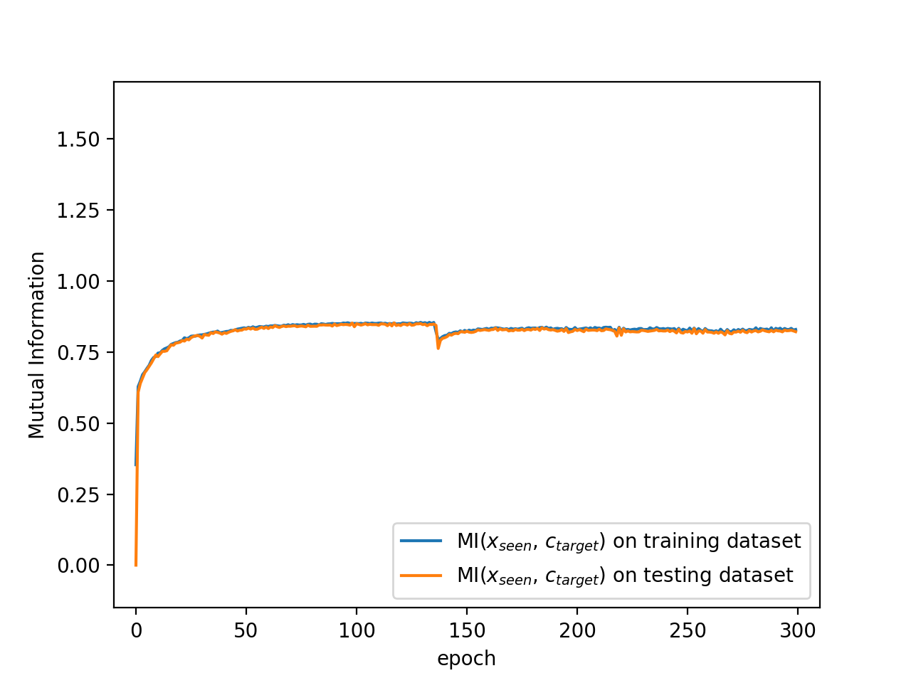
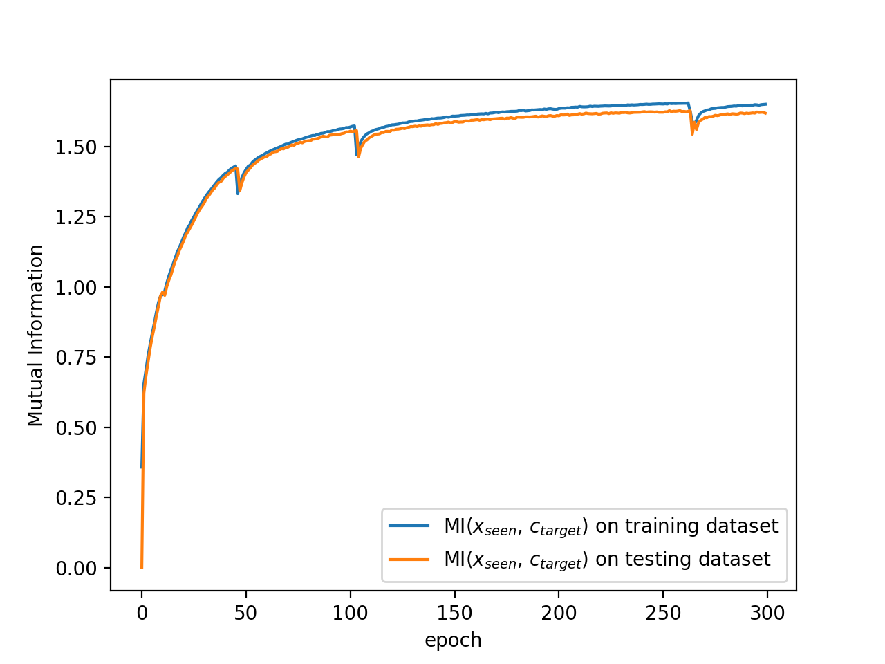
Figure 2: Trajectory of mutual information $\mathrm{MI}(x_{seen},c_{target})$: Left, the model is trained without the mutual information loss $L_{\mathrm{MI}}$; Right, the model is trained with the mutual information loss $L_{\mathrm{MI}}$.

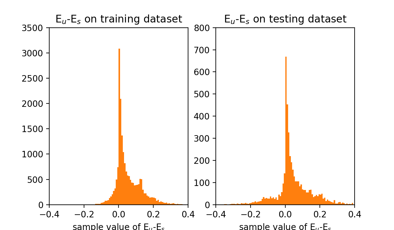
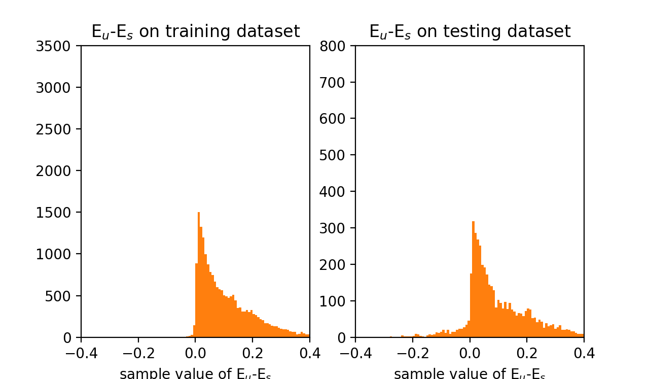
Figure 3: Sample histogram of the term $E_{u}-E_{s}$: Left, the model is trained without the entropy constraint loss $L_{\mathrm{EC}}$; Right, the model is trained with entropy constraint loss $L_{\mathrm{EC}}$.

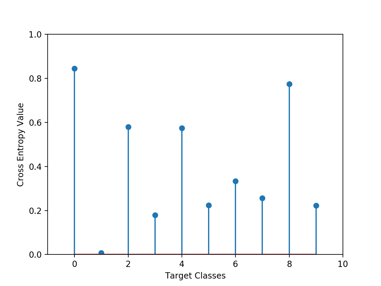
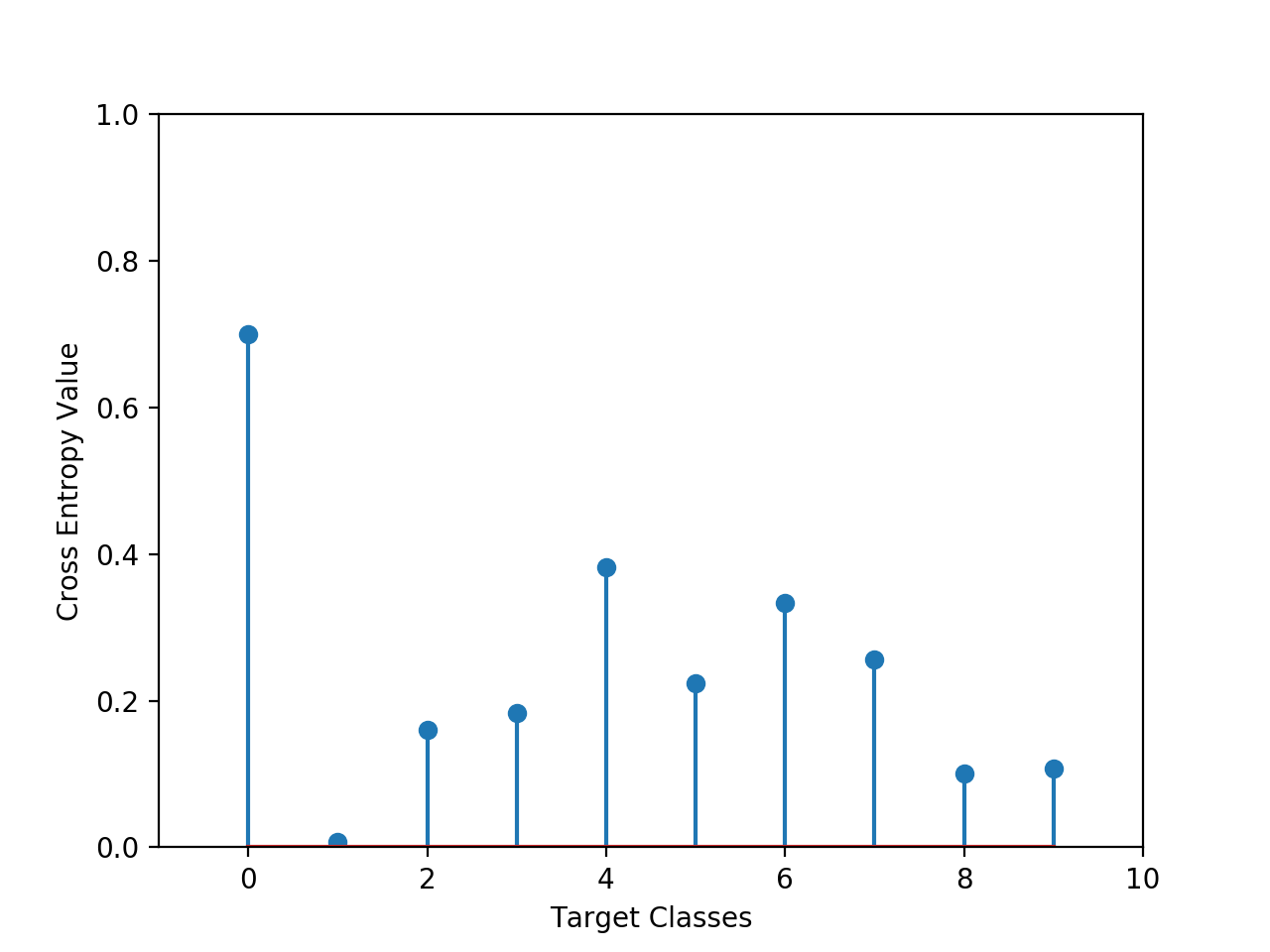
Figure 4: Cross entropy between PV representations of ten target classes representations $v_{i}^{t}$ (for $i\in\{1,...,10\}$) in the AwA1 dataset with respect to its forty source classes representations $v_{1:40}^{s}$, $CE(v_{i}^{t},v^{s}_{1:40},\psi)$: Left, the model is trained without the semantic preserving cross entropy loss $L_{\mathrm{SPCE}}$; Right, the model is trained with loss $L_{\mathrm{SPCE}}$.

Numerical evaluation on performance

We investigate contribution of our proposed approach on the model performance for GZSL. Here we use both the AwA1 and AwA2 datasets. We include the result of DCN model [27] on AwA2 and the prototypical model trained with only the cross entropy loss as baseline methods. We compare the choice of common embedding spaces, attribute space and feature space, and the choice of distances, cosine and dot product. We represent the combinations as follows: space A uses the attribute space as the embedding space and uses dot product similarity based distance; space B uses the visual space as the embedding space and uses cosine similarity based distance; space C uses the visual space as the embedding space and uses dot product similarity based distance. Notice that the last two rows in Tab. 1 also choose space C. Furthermore, we show the contribution of the proposed information-theoretic losses: $L_{\text{Ent}}$, $L_{\text{MI}}$, $L_{\text{EC}}$ and $L_{\text{SPCE}}$.

All the simulation results are shown in Tab. 1, where we cite the result of DCN directly from [27]. The DCN model introduces an entropy regularization for bridging seen data and target classes, which is similar with the $L_{\text{Ent}}$ (notice that we have an extra term $\mathrm{margin}_{1}$ in the Eq. 5). The DCN uses the dot product distance, and project the feature and attribute onto a common space. The third to the fifth rows show that the entropy loss $L_{\text{Ent}}$ significantly improves the GZSL performance, comparing to the cross entropy loss $L_{\text{CE}}$. And the results of the third to the fifth rows outperform the DCN significantly, which might be due to the factors that it is easier to train the model using the original attribute/feature space rather than looking for a common space, and the proposed entropy loss seems more effective than the entropy regularization in DCN. Furthermore, the third to the fifth rows demonstrate the importance of choosing the common embedding space and distance function: using the visual feature space rather than the semantic space as the embedding space gains strong improvement; using dot product similarity based distance yields better performances than using cosine similarity based distance. Comparing the sixth row with the fifth row, we show that the proposed marginal entropy $H(c)$ in $L_{\text{MI}}$ brings additional improvements. Comparing the results in the seventh row and sixth row, we show that the entropy constraint $L_{\text{EC}}$ can significantly boost the model performance. In the last row, we show that the semantic preserving loss $L_{\text{SPCE}}$ achieves a favorable improvement on AwA1 dataset but brings a negligible negative effect on AwA2 dataset. Experiments show that, for other datasets, the semantic preserving loss also make positive contributions, so we retain this loss in following simulation studies.

Table 1: Comparison of the contribution of different improvement approaches.

Methods	AwA1			AwA2
	ts	tr	H	ts	tr	H
DCN[27]	-	-	-	25.5	84.2	39.1
$L_{\text{CE}}$ (space C)	11.4	89.9	20.2	13.6	90.6	23.7
+$L_{\text{Ent}}$ (space A)	35.7	66.0	46.3	39.4	75.5	51.7
+$L_{\text{Ent}}$ (space B)	37.8	67.0	48.3	41.1	80.2	54.2
+$L_{\text{Ent}}$ (space C)	39.8	70.1	50.8	46.2	71.6	56.2
+$L_{\text{MI}}$ (space C)	39.3	72.9	51.1	49.5	70.9	58.2
+$L_{\text{MI}}$+$L_{\text{EC}}$	45.2	72.6	55.7	52.7	74.1	61.6
+$L_{\text{MI}}$+$L_{\text{EC}}$+$L_{\text{SPCE}}$	50.2	71.5	59.0	52.2	74.3	61.3

5.4 Conventional zero shot learning results

We investigate the proposed method for conventional ZSL that only recognize unseen classes at the test stage. And we compare the result of our method with several state of the art results from recent works [3][33][10][4][47]. As shown in Tab. 2, the proposed approach compares favorably with the existing approaches in literature, obtaining the state-of-the-art on SUN, AwA2 and aPY datasets. On CUB dataset, our result is 2% lower than DLFZRL [47].

Table 2: Results of Conventional Zero-Shot Learning.

Method	SUN	CUB	AwA2	aPY
DAP[25]	39.9	40.0	46.1	33.8
CONSE[31]	38.8	34.3	44.5	26.9
ALE[1]	58.1	54.9	62.5	39.7
DEVISE[15]	56.5	52.0	59.7	39.8
SJE[3]	53.7	53.9	61.9	32.9
ESZSL[33]	54.5	53.9	58.6	38.3
SYNC[10]	40.3	55.6	46.6	23.9
PSR[4]	61.4	56.0	63.8	38.4
DLFZRL[47]	59.3	57.8	63.7	44.5
Proposed	62.1	57.6	64.6	44.7

Table 3: Results of Generalized Zero-Shot Learning on four datasets under Proposed Splits (PS)[56]

Methods	AwA2			CUB			SUN			aPY
	ts	tr	H	ts	tr	H	ts	tr	H	ts	tr	H
Non-Generative Models
ALE[1]	16.8	76.1	27.5	23.7	62.8	34.4	21.8	33.1	26.3	4.6	73.7	8.7
DeViSE[15]	13.4	68.7	22.4	23.8	53.0	32.8	16.9	27.4	20.9	4.9	76.9	9.2
SynC[10]	8.9	87.3	16.2	11.5	70.9	19.8	7.9	43.3	13.4	7.4	66.3	13.3
ZSKL[59]	18.9	82.7	30.8	21.6	52.8	30.6	20.1	31.4	24.5	10.5	76.2	18.5
DCN [27]	25.5	84.2	39.1	28.4	60.7	38.7	25.5	37.0	30.2	14.2	75.0	23.9
DLFZRL [47]	-	-	45.1	-	-	37.1	-	-	24.6	-	-	31.0
Proposed	52.7	74.1	61.6	40.6	55.1	46.7	41.7	37.4	39.5	31.5	51.8	39.2
Generative Models
f-CLSWGAN[55]	52.1	68.9	59.4	43.7	57.7	49.7	42.6	36.6	39.4	-	-	-
F-VAEGAN-D2[57]	57.6	70.6	63.5	48.4	60.1	53.6	45.1	38.0	41.3	-	-	-
CADA-VAE[39]	55.8	75.0	63.9	51.6	53.5	52.4	47.2	35.7	40.6	-	-	-
CRnet[58]	52.6	52.6	63.1	45.5	56.8	50.5	34.1	36.5	35.3	32.4	68.4	44.0
DLFZRL+softmax[47]	-	-	60.9	-	-	51.9	-	-	42.5	-	-	38.5
TCN [20]	61.2	65.8	63.4	52.6	52.0	52.3	31.2	37.3	34.0	24.1	64.0	35.1
GDAN [19]	32.1	67.5	43.5	39.3	66.7	49.5	38.1	89.9	53.4	30.4	75.0	43.4
IZF [40]	60.6	77.5	68.0	52.7	68.0	59.4	52.7	57.0	54.8	42.3	60.5	49.8
DVBE [29]	62.7	77.5	69.4	64.4	73.2	68.5	44.1	41.6	42.8	37.8	55.9	45.2
IAS [12]	65.1	78.9	71.3	41.4	49.7	45.2	29.9	40.2	34.3	35.1	65.5	45.7
f-CLSWGAN+Proposed	56.4	83.2	67.2	52.1	55.8	53.9	53.3	35.0	42.3	37.1	57.7	45.2

5.5 Generalized zero shot learning results

Comparison with deterministic models

We compare the performance of our proposed model with several recent deterministic models for GZSL. Taking DCN [27] as the baseline model, as shown in Tab. 3, our method gains a superior accuracy compared to other deterministic models on all datasets: it obtains $21\%\thicksim 64\%$ improvements over DCN and significantly outperforms a previous state-of-art deterministic model-DLFZRL [47]. Besides, we observe that our deterministic model obtains superior results than some generative models, for example, it outperforms the f-CLSWGAN on all datasets.

Comparison with generative models

We investigate the performance of our proposed method by incorporating a generative model, f-CLSWGAN. Seen image features and class-level attributes are used to train f-CLSWGAN and image features of unseen classes can be generated by unseen class-level attributes. Including the generated features for target classes into the entire training, we train the model by the loss function defined in Sec. 4.4. As shown in Tab. 3, our proposed model significantly outperforms the baseline model f-CLSWGAN with $7\%\thicksim 13\%$ improvements. Our proposed method achieve comparable results with several recently proposed sophisticated generative models. Moreover, unlike some generative models, such as [20, 19, 12] gain superior results on one or two datasets but inferior results on other dataset, our proposed method obtain favorable results on all the dataset: it ranks as the top 3 $\thicksim$ top 5 method for each dataset.

6 Conclusion

This paper addresses information-theoretic loss functions to quantify the knowledge transfer and semantic relation for GZSL/ZSL. Leveraging on the proposed probability vector representation based on the prototypical model, the proposed loss can be effectively evaluated with simple closed forms. Experiments show that our approach yields state of the art performance for deterministic approach for GZSL and conventional ZSL tasks. Moreover, by incorporating with generated data from f-CLSWGAN, the proposed method also gains favorable performance. One limitation of this work is that we need pretty much extra cross validation to select the hyperparameters; Another limitation is that the loss functions have certain correlation, so further study is needed to simply the loss functions while keeping similar performance, and reduce the number of hyperparameters.

References

- [1] Zeynep Akata, Florent Perronnin, Zaid Harchaoui, and Cordelia Schmid. Label-embedding for attribute-based classification. In IEEE Transactions on Computer Vision and Pattern Recognition, pages 819–826, 2013.
- [2] Zeynep Akata, Florent Perronnin, Zaid Harchaoui, and Cordelia Schmid. Label-embedding for image classification. In IEEE Transactions on Pattern Analysis and Machine Intelligence, pages 1425–1438, 2016.
- [3] Zeynep Akata, Scott E. Reed, Daniel Walter, Honglak Lee, and Bernt Schiele. Evaluation of output embeddings for fine grained image classification. In IEEE Transactions on Computer Vision and Pattern Recognition, pages 2927–2936, 2015.
- [4] Y. Annadani and S. Biswas. Preserving semantic relations for zero-shot learning. In Proceedings of the IEEE Conference on Computer Visionand Pattern Recognition, pages 7603–7612, 2018.
- [5] Martín Arjovsky and L. Bottou. Towards principled methods for training generative adversarial networks. ArXiv, abs/1701.04862, 2017.
- [6] Martín Arjovsky, Soumith Chintala, and Léon Bottou. Wasserstein gan. ArXiv, abs/1701.07875, 2017.
- [7] Jianmin Bao, D. Chen, Fang Wen, H. Li, and G. Hua. Cvae-gan: Fine-grained image generation through asymmetric training. 2017 IEEE International Conference on Computer Vision (ICCV), pages 2764–2773, 2017.
- [8] Yoshua Bengio, Aaron C. Courville, and Pascal Vincent. Representation learning: A review and new perspectives. In IEEE Transactions on Pattern Analysis and Machine Intelligence, pages 1798–1828, 2013.
- [9] Yannick Le Cacheux, H. Borgne, and M. Crucianu. Modeling inter and intra-class relations in the triplet loss for zero-shot learning. 2019 IEEE/CVF International Conference on Computer Vision (ICCV), pages 10332–10341, 2019.
- [10] Soravit Changpinyo, Wei-Lun Chao, Boqing Gong, and Fei Sha. Synthesized classifiers for zero-shot learning. In IEEE Transactions on Computer Vision and Pattern Recognition, pages 5327–5336, 2016.
- [11] W.-L. Chao, S. Changpinyo, B. Gong, and F. Sha. An empirical study and analysis of generalized zero-shot learning for object recognitionin the wild. In European Conference on Computer Vision, pages 52–68, 2016.
- [12] Yu-Ying Chou, Hsuan-Tien Lin, and Tyng-Luh Liu. Adaptive and generative zero-shot learning. In ICLR, 2021.
- [13] Jia Deng, W. Dong, R. Socher, L. Li, K. Li, and Li Fei-Fei. Imagenet: A large-scale hierarchical image database. In CVPR, 2009.
- [14] A. Farhadi, I. Endres, D. Hoiem, and D. Forsyth. Describing objects by their attributes. In IEEE Conference on Computer Vision and Pattern Recognition, 2009.
- [15] Andrea Frome, Greg S Corrado, Jon Shlens, Samy Bengio, Jeff Dean, Marc Aurelio Ranzato, and Tomas Mikolov. Devise:a deep visual-semantic embedding model. In Conference and Workshop on Neural Information Processing Systems, pages 2121–2129, 2013.
- [16] Y. Fu, T. M. Hospedales, T. Xiang, and S. Gong. Transductive multi-view zero-shot learning. In IEEE Transactions on Pattern Analysis and Machine Intelligence, volume 37, pages 2332–2345, 2015.
- [17] I. Goodfellow, J. Pouget-Abadie, M. Mirza, B. Xu, D. Warde-Farley, S. Ozair, A. Courville, and Y. Bengio. Generative adversarial nets. In Conference and Workshop on Neural Information Processing Systems, pages 2672–2680, 2014.
- [18] K. He, X. Zhang, S. Ren, and J. Sun. Deep residual learning for image recognition. In Proceedings of the IEEE Conference on Computer Visionand Pattern Recognition, pages 770–778, 2016.
- [19] He Huang, Changhu Wang, Philip S. Yu, and Chang-Dong Wang. Generative dual adversarial network for generalized zero-shot learning. 2019 IEEE/CVF Conference on Computer Vision and Pattern Recognition (CVPR), pages 801–810, 2019.
- [20] Huajie Jiang, Ruiping Wang, S. Shan, and Xilin Chen. Transferable contrastive network for generalized zero-shot learning. 2019 IEEE/CVF International Conference on Computer Vision (ICCV), pages 9764–9773, 2019.
- [21] Rohit Keshari, R. Singh, and Mayank Vatsa. Generalized zero-shot learning via over-complete distribution. 2020 IEEE/CVF Conference on Computer Vision and Pattern Recognition (CVPR), pages 13297–13305, 2020.
- [22] Diederik P. Kingma and Jimmy Ba. Adam: A method for stochastic optimization. CoRR, abs/1412.6980, 2015.
- [23] Diederik P. Kingma and Max Welling. Auto-encoding variational bayes. In International Conference on Learning Representations, 2014.
- [24] A. Krizhevsky, I. Sutskever, and G. E. Hinton. Imagenet classification with deep convolutional neuralnetworks. In Conference and Workshop on Neural Information Processing Systems, 2012.
- [25] C. H. Lampert, H. Nickisch, and S. Harmeling. Attribute-based classification for zero-shot visual object categorization. In IEEE Transactions on Pattern Analysis and Machine Intelligence, volume 36, pages 453–465, 2014.
- [26] A. Lazaridou, Georgiana Dinu, and Marco Baroni. Hubness and pollution: Delving into cross-space mapping for zero-shot learning. In ACL, 2015.
- [27] S. Liu, M. Long, J. Wang, and M. I. Jordan. Generalized zero-shot learning with deep calibration network. In Neural InformationProcessing Systems, 2018.
- [28] Tomas Mikolov, Kai Chen, Greg Corrado, and Jeffrey Dean. Efficient estimation of word representations in vector space. In International Conference on Learning Representations, 2013.
- [29] Shaobo Min, Hantao Yao, Hongtao Xie, Chaoqun Wang, Zhengjun Zha, and Yongdong Zhang. Domain-aware visual bias eliminating for generalized zero-shot learning. 2020 IEEE/CVF Conference on Computer Vision and Pattern Recognition (CVPR), pages 12661–12670, 2020.
- [30] Ashish Mishra, M. K. Reddy, Anurag Mittal, and H. Murthy. A generative model for zero shot learning using conditional variational autoencoders. 2018 IEEE/CVF Conference on Computer Vision and Pattern Recognition Workshops (CVPRW), pages 2269–22698, 2018.
- [31] Norouzi Mohammad, Mikolov Tomas, Bengio Samy, SingerYoram, Shlens Jonathon, Frome Andrea, Corrado Greg, and Dean Jeffrey. Zero-shot learning by convex combination of semantic embeddings. In International Conference on Learning Representations, 2014.
- [32] M. Palatucci, D. Pomerleau, G. E. Hinton, and T. M. Mitchell. Zero-shot learning with semantic outputcodes. In Conference and Workshop on Neural Information Processing Systems, pages 1410–1418, 2009.
- [33] B. Romera Paredes and P. Torr. An embarrassingly simple approach to zero-shot learning. In International Conference on Machine Learning, pages 2152–2161, 2015.
- [34] Adam Paszke, S. Gross, Soumith Chintala, Gregory Chanan, Edward Yang, Zach DeVito, Zeming Lin, Alban Desmaison, L. Antiga, and A. Lerer. Automatic differentiation in pytorch. 2017.
- [35] G. Patterson and J. Hays. Sun attribute database: Discovering, annotating,and recognizing scene attributes. In IEEE Conference on Computer Vision and Pattern Recognition, pages 2751–2758, 2012.
- [36] M. Radovanović, A. Nanopoulos, and M. Ivanovic. Hubs in space: Popular nearest neighbors in high-dimensional data. J. Mach. Learn. Res., 11:2487–2531, 2010.
- [37] S. Ravi and H. Larochelle. Optimization as a model for few-shot learning. In ICLR, 2017.
- [38] D. E. Rumelhart, G. E. Hinton, and R. J. Williams. Parallel distributed processing: Explorations in themicrostructure of cognition. MIT Press, 1, 1986.
- [39] E. Schonfeld, S. Ebrahimi, S. Sinha, T. Darrell, and Z. Akata. Generalized zero and few-shot learning via aligned variational autoencoders. In Proceedings of the IEEE Conference on Computer Vision and Pattern Recognition, 2019.
- [40] Yuming Shen, Jie Qin, and Lei Huang. Invertible zero-shot recognition flows. ArXiv, abs/2007.04873, 2020.
- [41] Yutaro Shigeto, Ikumi Suzuki, Kazuo Hara, MasashiShimbo, and Yuji Matsumoto. Ridge regression, hubness,and zero-shot learning. In The European Conference on Machine Learning and Principles and Practice of Knowledge Discovery in Databases, pages 135–151, 2015.
- [42] K. Simonyan and A. Zisserman. Very deep convolutional networks for large scale image recognition. In International Conference on Learning Representations, 2015.
- [43] J. Snell, Kevin Swersky, and R. Zemel. Prototypical networks for few-shot learning. In NIPS, 2017.
- [44] R. Socher, M. Ganjoo C. D. Manning, and A. Ng. Zero-shot learning through cross-modal transfer. In Proceeding of Neural Information Processing Systems, 2013.
- [45] Kihyuk Sohn, H. Lee, and Xinchen Yan. Learning structured output representation using deep conditional generative models. In NIPS, 2015.
- [46] N. Tomasev, M. Radovanovic, D. Mladenic, and M. Ivanovic. The role of hubness in clustering high-dimensional data. IEEE Transactions on Knowledge and Data Engineering, 26(3):739–751, 2014.
- [47] Bin Tong, Chao Wang, Martin Klinkigt, Yoshiyuki Kobayashi, and Yuuichi Nonaka. Hierarchical disentanglement of discriminative latent features for zero-shot learning. 2019 IEEE/CVF Conference on Computer Vision and Pattern Recognition (CVPR), pages 11459–11468, 2019.
- [48] Y. H. Tsai, L. Huang, and R. Salakhutdinov. Learning robust visual-semantic embeddings. In IEEE International Conference on Computer Vision, pages 3591–3600, 2017.
- [49] Oriol Vinyals, C. Blundell, T. Lillicrap, K. Kavukcuoglu, and Daan Wierstra. Matching networks for one shot learning. In NIPS, 2016.
- [50] C. Wah, S. Branson, P. Welinder, P. Perona, and S. Belongie. The caltech-ucsd birds-200-2011 dataset. 2011.
- [51] W. Wang, V. Zheng, H. Yu, and C. Miao. A survey of zero-shot learning. ACM Transactions on Intelligent Systems and Technology (TIST), 10:1 – 37, 2019.
- [52] Z. Wu, Y. Fu, Y.-G. Jiang, and L. Sigal. Harnessing object and scene semantics for large-scale video understanding. In IEEE Transactions on Computer Vision and Pattern Recognition, pages 3112–3121, 2016.
- [53] Y. Xian, Z. Akata, G. Sharma, Q. Nguyen, M. Hein, and B. Schiele. Latent embeddings for zero-shot classification. In Proceedings of theIEEE Conference on Computer Vision and Pattern Recognition, pages 69–77, 2016.
- [54] Y. Xian, C. H. Lampert, B. Schiele, and Z. Akata. Zero-shot learninga comprehensive evaluation of the good, the bad and the ugly. In IEEE Transactions on Pattern Analysis and Machine Intelligence, 2018.
- [55] Y. Xian, T. Lorenz, B. Schiele, and Z. Akata. Feature generating networks for zero-shot learning. In Proceedings of the IEEE Conferenceon Computer Vision and Pattern Recognition, 2018.
- [56] Y. Xian, B. Schiele, and Z. Akata. Zero-shot learning-the good, the bad and the ugly. In Proceedings of the IEEE Conference on ComputerVision and Pattern Recognition, pages 4582–4591, 2017.
- [57] Yongqin Xian, Saurabh Sharma, Bernt Schiele, and Zeynep Akata. F-vaegan-d2: A feature generating framework for any-shot learning. 2019 IEEE/CVF Conference on Computer Vision and Pattern Recognition (CVPR), pages 10267–10276, 2019.
- [58] Fei Zhang and Guangming Shi. Co-representation network for generalized zero-shot learning. In ICML, 2019.
- [59] H. Zhang and P. Koniusz. Zero-shot kernel learning. In Proceedings of the IEEE Conference on Computer Vision and Pattern Recognition, 2018.
- [60] L. Zhang, P. Wang, L. Liu, C. Shen, W. Wei, Y. Zhang, and A. V. D.Hengel. Towards effective deep embedding for zero-shot learning. ArXiv preprint,arXiv:1808.10075, 2018.
- [61] L. Zhang, T. Xiang, and S. Gong. Learning a deep embedding model for zero-shot learning. In Proceedings of the IEEE Conference on Computer Vision and Pattern Recognition, pages 2021–2030, 2017.
- [62] Z. Zhang and V. Saligrama. Zero-shot learning via semantic similarity embedding. In Proceedings of the IEEE International Conference on Computer Vision, pages 4166–4174, 2015.