Abstract

Invariant finite-difference schemes are considered for one-dimensional magnetohydrodynamics (MHD) equations in mass Lagrangian coordinates for the cases of finite and infinite conductivity. The construction of these schemes make use of previously obtained results of the group classification of MHD equations Dorodnitsyn et al. (2022). On the basis of the classical Samarskiy–Popov scheme, new schemes are constructed for the case of finite conductivity. These schemes admit all symmetries of the original differential model and have difference analogues of all of its local differential conservation laws. New, previously unknown, conservation laws are found using symmetries and direct calculations. In the case of infinite conductivity, conservative invariant schemes are constructed as well. For isentropic flows of a polytropic gas the proposed schemes possess the conservation law of energy and preserve entropy on two time layers. This is achieved by means of specially selected approximations for the equation of state of a polytropic gas. Also, invariant difference schemes with additional conservation laws are proposed. A new scheme for the case of finite conductivity is tested numerically for various boundary conditions which shows accurate preservation of difference conservation laws.

1 1 0 https://doi.org/ Invariant Finite-Difference Schemes With Conservation Laws Preservation For One-Dimensional MHD Equations Invariant Schemes For MHD Evgeniy Kaptsov ${}^{1,\textmd{*}}$, Vladimir Dorodnitsyn ² Evgeniy Kaptsov, Vladimir Dorodnitsyn Kaptsov, E.; Dorodnitsyn, V. Correspondence: evgkaptsov@gmail.com

1 Introduction

Magnetic hydrodynamics equations describe the flows of electrically conductive fluids such as plasma, liquid metals, and electrolytes and are widely used in modeling processes in various fields from engineering to geophysics and astrophysics.

In the present publication, we restrict ourselves to considering plane one-dimensional MHD flows under the assumption that the medium is inviscid and thermally non-conducting. A group classification of the MHD equations under the above conditions was carried out recently in Dorodnitsyn et al. (2022) (for some particular results see also Gridnev (1968); Dorodnitsyn (1976); Rogers (1969); Ibragimov (1995)). The group classification splits into four essentially different cases according to whether the conductivity of the medium is finite or infinite, and the longitudinal component of the magnetic field vector is zero or a non-zero constant.

The MHD equations are nonlinear, so that even in the one-dimensional case only their particular solutions are known Oliveri and M.P. (2005); Picard (2008); Golovin (2019, 2011); Golovin and Sesma (2019). Therefore, numerical modeling in magnetohydrodynamics is of great practical interest. There are many approaches to numerically modeling MHD equations, including finite-difference, finite element and finite volume methods (see, e.g. Toro (1997); Samarskiy and Popov (1970); Samarskii and Popov (1980); Falle et al. (1998); Powell et al. (1999); Yakovlev et al. (2013); Yang et al. (2017); Hirabayashi et al. (2016); Ryu and Jones (1995)). Further we consider finite-difference schemes taking as a starting point the classical Samarsky–Popov schemes Samarskiy and Popov (1970); Samarskii and Popov (1980) for the MHD equations for the case of finite conductivity. The main properties of the considered schemes are invariance, i.e. preservation of the symmetries of the original differential equations, and the presence of difference analogues of local differential conservation laws. It is known that there is a connection between the invariance of equations and the presence of conservation laws Noether (1918); Ibragimov (1985); Olver (1986); Bluman and Anco (2002).

Invariant schemes have been studied for a long time Dorodnitsyn (1991, 1994); Maeda (1985, 1987); Dorodnitsyn (2011), and over the past decades, significant progress has been made in the development of methods for their construction and integration. For schemes for ordinary differential equations with Lagranagian or Hamiltonian functions, a number of methods Dorodnitsyn et al. (2004, 2003); Dorodnitsyn and Kozlov (2009, 2010) have been developed that make it possible to decrease the order or even integrate the schemes. A method based on the Lagrangian identity has also been developed for the case when the equations do not admit a variational formulation Winternitz et al. (2014); Dorodnitsyn et al. (2015).

For partial difference schemes, the main methods used are the method of differential invariants Dorodnitsyn (2011); Bourlioux et al. (2006, 2007) and the difference analogue of the direct method Dorodnitsyn (2011); Cheviakov et al. (2020). Using these methods, the authors have constructed invariant schemes for various shallow water models Dorodnitsyn and Kaptsov (2020); Dorodnitsyn et al. (2020); Dorodnitsyn and Kaptsov (2021); Kaptsov et al. (2021). Also, some previously known schemes have been investigated from a group analysis point of view. In particular, symmetries and conservation laws of the Samarskiy–Popov schemes for the one-dimensional gas dynamics equations of a polytropic gas have been investigated in Dorodnitsyn et al. (2019); Kozlov (2019); Dorodnitsyn et al. (2021). Based on the results of the group classification Dorodnitsyn et al. (2022) and Samarskiy–Popov schemes for the MHD equations, we further construct invariant finite-difference schemes possessing conservation laws. The set and number of conservation laws depend on the conductivity, the form of the magnetic field vector and the equation of state of the medium.

This paper is organized as follows. In Section 2 the simplest version of the finite-conductivity MHD equations in mass Lagrangian coordinates in case of one-dimensional plane flows is considered. Electric and magnetic fields are represented by one-component vectors, which greatly simplifies the form of the equations. This was the main case considered in Samarsky and Popov’s publications Samarskiy and Popov (1970); Samarskii and Popov (1980). The section also provides basic notation and definitions. Then, symmetries and conservation laws of the Samarsky-Popov scheme for the MHD equations are investigated. In addition to the previously known conservation laws, the center-of-mass conservation law is given, as well as new conservation laws for the specific conductivity function, obtained on the basis of the group classification Dorodnitsyn et al. (2022).

Section 3 is devoted to various generalizations of the scheme of Section 2. In Section 3.1 the scheme for arbitrary electric and magnetic fields is considered. Its symmetries are investigated and conservation laws are given. The case of infinite conductivity is considered in Section 3.2. It is shown that in this case the Samarsky-Popov scheme requires some additional modifications in order to possess the conservation law of angular momentum. In the case of a polytropic gas, it turns out to be possible to preserve not only energy, but also entropy along pathlines. This can be done using a specially selected equation of state for a polytropic gas. At the end of the section, an example of an invariant scheme is given that does not possess a conservation law of energy, but preserves entropy and has additional conservation laws in the case of isentropic flows. In Section 4, one of the invariant schemes for the case of finite conductivity is numerically implemented for the example of plasma bunch deceleration by crossed electromagnetic fields. The results are discussed in the Conclusion.

2 Conservative schemes for MHD equations with finite conductivity

Problems of continuum mechanics and plasma physics are often considered in mass Lagrangian coordinates  Samarskii and Popov (1980); Rojdestvenskiy and Yanenko (1968) since for them the formulation of boundary conditions is greatly simplified. In particular, the conservative Samarsky–Popov schemes for the equations of gas dynamics and magnetohydrodynamics have been constructed in mass Lagrangian coordinates.

In mass Lagrangian coordinates the MHD equations, describing the plane one-dimensional MHD flows, are Samarskii and Popov (1980); Dorodnitsyn et al. (2022)

$$\left(\frac{1}{\rho}\right)_{t}=u_{s},$$ (1a)

$$u_{t}=-\left(p+\frac{(H^{y})^{2}+(H^{z})^{2}}{2}\right)_{s},$$ (1b)

$$v_{t}=H^{0}H^{y}_{{s}},\qquad y_{t}=v,$$ (1c)

$$w_{t}=H^{0}H^{z}_{{s}},\qquad z_{t}=w,$$ (1d)

$$\left(\frac{H^{y}}{\rho}\right)_{t}=(H^{0}v+E^{z})_{s},$$ (1e)

$$\left(\frac{H^{z}}{\rho}\right)_{t}=(H^{0}w-E^{y})_{s},$$ (1f)

$$\sigma E^{y}=-\rho H^{z}_{{s}},\qquad\sigma E^{z}=\rho H^{y}_{{s}},$$ (1g)

$$\varepsilon_{t}=-pu_{s}+\frac{1}{\rho}(\mathbf{i}\cdot\mathbf{E}),$$ (1h)

$$x_{t}=u,\qquad x_{s}=1/\rho,$$ (1i)

where $t$ is time, $s$ is mass Lagrangian coordinate, $x$ is Eulerian coordinate, $\rho$ is density, $p$ is pressure, $\varepsilon$ is internal energy, $\mathbf{u}=(u,v,w)$ is the velocity of a particle, $\mathbf{E}=(E^{x},E^{y},E^{z})$ is the electric field vector, $\mathbf{H}=(H^{x},H^{y},H^{z})$ is the magnetic field vector, and $\mathbf{i}=(i^{x},i^{y},i^{z})$ is the electric current. The conductivity $\sigma$ is some function of $p$ and $\rho$, i.e., $\sigma=\sigma(p,\rho)$.

Following Samarskii and Popov (1980) we firstly consider the simplest case of one-component electric and magnetic fields. Here we also introduce the notation and some basic concepts. In the next section some generalizations are considered, including the case of infinite conductivity.

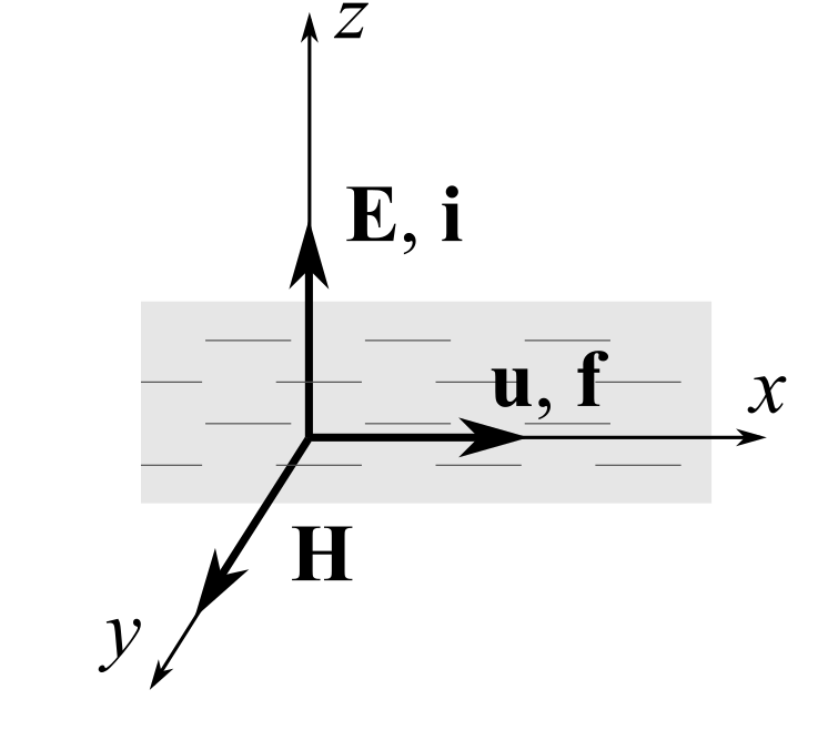
Figure 1: A plane one-dimensional flow for the chosen coordinates

For simplicity, the longitudinal component of the magnetic field $\mathbf{H}$ is set to zero, and the coordinate system is chosen in such a way that $\mathbf{H}=(0,H,0)$. Consequently, the electric current $\mathbf{i}$ and the electric field $\mathbf{E}$ are also one-component vectors, i.e., $\mathbf{i}=(0,0,i)$, $\mathbf{E}=(0,0,E)$. Electromagnetic force $\mathbf{f}=(f,0,0)$ acts in the $x$-direction, and the velocity is $\mathbf{u}=(u,0,0)$ (see Figure 1).

Given the above, the system of the one-dimensional MHD equations with a finite conductivity $|\sigma|<\infty$ in mass Lagrangian coordinates can be written as Samarskii and Popov (1980)

$$\left(\frac{1}{\rho}\right)_{t}=u_{s},$$ (2a)

$$u_{t}=-p_{s}+f,\qquad f=-iH/\rho,$$ (2b)

$$\left(\frac{H}{\rho}\right)_{t}=E_{s},$$ (2c)

$$i=\sigma E=\kappa{\rho}H_{s},$$ (2d)

$$\varepsilon_{t}=-pu_{s}+q,\qquad q=iE/\rho,$$ (2e)

$$x_{t}=u,\qquad x_{s}=1/\rho,$$ (2f)

where $\kappa=1/(4\pi)$ and $q$ is Joule heating per unit mass.

In particular, we consider a polytropic gas for that the following relation holds

$$\varepsilon=\frac{1}{\gamma-1}\frac{p}{\rho},\qquad\gamma=\text{const}>1.$$ (3)

Equation (2e) for the energy evolution can be rewritten in the semi-divergent form

$$\left(\varepsilon+\frac{u^{2}}{2}\right)_{t}=-(pu)_{s}+fu+q,$$ (4)

or in the divergent form

$$\left(\varepsilon+\frac{u^{2}}{2}+\kappa\frac{H^{2}}{2\rho}\right)_{t}=-\left[\left(p+\kappa\frac{H^{2}}{2}\right)u\right]_{s}+\kappa\left(EH\right)_{s}.$$ (5)

Notice that the electromagnetic force $f=-iH/\rho$ can be represented in the divergent form $f=-\kappa(H^{2}/2)_{s}$, and equation (2b) can be rewritten as

$$u_{t}=-\left(p+\kappa\frac{H^{2}}{2}\right)_{s}.$$ (6)

Further we assume $\kappa=1$ since it can be discarded by means of the scaling transformation

$$\tilde{s}=\kappa s,\quad\tilde{p}=\kappa p,\quad\tilde{\rho}=\kappa\rho,\quad\tilde{\sigma}=\kappa\sigma.$$ (7)

2.1 Conservative Samarskiy–Popov’s schemes for system (2)

The family of Samarskiy–Popov’s conservative difference schemes for system (2) is

$$\left(\frac{1}{\rho}\right)_{t}=u_{s}^{(0.5)},$$ (8a)

$$u_{t}=-p^{(\alpha)}_{\bar{s}}+f,\qquad f=-\left(\frac{H\hat{H}}{2}\right)_{\bar{s}}=-\frac{1}{2}[\hat{i}H_{*}/\hat{\rho}_{*}+i\hat{H}_{*}/\rho_{*}],$$ (8b)

$$\left(\frac{H}{\rho}\right)_{t}=E_{s}^{(\beta)},$$ (8c)

$$i=\sigma_{*}E=\rho_{*}H_{\bar{s}},$$ (8d)

$$\varepsilon_{t}=-p^{(\alpha)}u_{s}^{(0.5)}+q,\qquad q=\frac{1}{2}[(i/\rho_{*})^{(0.5)}E^{(\beta)}+(i_{+}/(\rho_{+})_{*})^{(0.5)}E_{+}^{(\beta)}],$$ (8e)

$$x_{t}=u^{(0.5)},\qquad x_{s}=\frac{1}{\rho},$$ (8f)

where $0\leqslant(\alpha,\beta)\leqslant 1$ are free parameters. For arbitrary $\alpha$ and $\beta$ scheme (8) approximates system (2) up to $O(\tau+h^{2})$, and for $\alpha=\beta=0.5$ the scheme is of order $O(\tau^{2}+h^{2})$.

Here and further $\phi_{t}$, $\phi_{\check{t}}$ and $\phi_{s}$, $\phi_{\bar{s}}$ denote finite-difference derivatives of some quantity $\phi=\phi(t_{n},s_{m},u^{n}_{m},...)$

$$\begin{array}[]{c}\displaystyle\phi_{t}=\frac{\mathop{S}\limits_{+\tau}(\phi)-\phi}{\tau_{n}},\qquad\phi_{s}=\frac{\mathop{S}\limits_{+s}(\phi)-\phi}{h_{m}},\\ \displaystyle\phi_{\check{t}}=\frac{\phi-\mathop{S}\limits_{-\tau}(\phi)}{\tau_{n-1}},\qquad\phi_{\bar{s}}=\frac{\phi-\mathop{S}\limits_{-s}(\phi)}{h_{m-1}},\end{array}$$ (9)

which are defined with the help of the finite-difference right and left shifts along the time and space axes correspondingly

$$\begin{array}[]{c}\displaystyle\underset{\pm\tau}{S}(\phi(t_{n},s_{m},u^{n}_{m},...))=\phi(t_{n\pm 1},s_{m},u^{n\pm 1}_{m},...),\\ \displaystyle\underset{\pm{s}}{S}(\phi(t_{n},s_{m},u^{n}_{m},...))=\phi(t_{n},s_{m\pm 1},u^{n}_{m\pm 1},...).\end{array}$$

The indices $n$ and $m$ are respectively changed along time and space axes $t$ and $s$. The time and space steps are defined as follows

$$\begin{array}[]{c}\displaystyle\tau_{n}=\hat{\tau}=t_{n+1}-t_{n}=\hat{t}-t,\qquad\tau_{n-1}=\check{\tau}=t_{n}-t_{n-1}=t-\check{t},\\ \displaystyle h_{m}=h_{+}=s_{m+1}-s_{m}=s_{+}-s,\qquad h_{m-1}=h_{-}=s_{m}-s_{m-1}=s-s_{-}.\end{array}$$ (10)

Following the Samarskiy–Popov notation throughout the text we denote

$$\mathop{S}\limits_{+s}(\phi)=\phi_{+},\quad\mathop{S}\limits_{-s}(\phi)=\phi_{-},\quad\mathop{S}\limits_{+\tau}(\phi)=\hat{\phi},\quad\mathop{S}\limits_{-\tau}(\phi)=\check{\phi},$$ (11)

$${\phi}^{(\alpha)}=\alpha\hat{{\phi}}+(1-\alpha){\phi}$$ (12)

and

$${\phi}_{*}=({\phi}_{*})^{j}_{i}=\frac{h_{i}{\phi}^{j}_{i-1/2}+h_{i-1}{\phi}^{j}_{i+1/2}}{h_{i}+h_{i-1}}.$$ (13)

Notice that on a uniform lattice $h_{i}=h=\text{const}$ in its integral nodes (13) becomes

$${\phi}_{*}=\frac{{\phi}_{-}+{\phi}}{2}.$$ (14)

The energy equation (8e) can be reduced to one of the three following forms Samarskii and Popov (1980) using equivalent algebraic transformations:

$$\varepsilon_{t}=-p^{(\alpha)}u_{s}^{(0.5)}+q,$$ (15)

$$\left(\varepsilon+\frac{u^{2}+u_{+}^{2}}{4}\right)_{t}=-\left(p_{*}^{(\alpha)}u^{(0.5)}\right)_{s}+\frac{1}{2}\left[fu^{(0.5)}+f_{+}u_{+}^{(0.5)}\right]+q,$$ (16)

$$\left(\varepsilon+\frac{u^{2}+u_{+}^{2}}{4}+\frac{H^{2}}{2\rho}\right)_{t}+\left[\left(p_{*}^{(\alpha)}+\frac{(H\hat{H})_{*}}{2}\right)u^{(0.5)}-E^{(\beta)}H_{*}^{(0.5)}\right]_{s}=0.$$ (17)

These different forms of equation reflect the balance of certain types of energy, i.e. they express the different physical aspects of energy conservation. To emphasize this property, such schemes are also called completely conservative.

2.2 Invariance of Samarskiy–Popov’s schemes

System (2) can be rewritten in the following form that is more convenient for symmetry analysis

$$\left(\frac{1}{\rho}\right)_{t}=u_{s},$$ (18a)

$$u_{t}=-\left(p+\frac{H^{2}}{2}\right)_{s},$$ (18b)

$$\left(\frac{H}{\rho}\right)_{t}=E_{s},$$ (18c)

$$\sigma E=\rho H_{s},$$ (18d)

$$p_{t}=-\gamma\rho pu_{s}+(\gamma-1)\sigma E^{2},$$ (18e)

$$x_{t}=u,\qquad x_{s}=1/\rho.$$ (18f)

Notice that for the polytropic gas with the state equation (3) one can rewrite the energy evolution equation (8e) of the Samarskiy–Popov scheme as

$$p_{t}=-\hat{\rho}(p+(\gamma-1)p^{(\alpha)})u^{(0.5)}+(\gamma-1)\frac{\hat{\rho}}{2}\left[\left(\frac{\sigma_{*}E}{\rho_{*}}\right)^{(0.5)}E^{(\beta)}+\left(\frac{(i_{+})_{*}E_{+}}{(\rho_{+})_{*}}\right)^{(0.5)}E_{+}^{(\beta)}\right].$$ (19)

In this form the energy evolution equation corresponds to equation (18e).

Calculations show Dorodnitsyn et al. (2022) that the Lie algebra admitted by the system for an arbitrary $\sigma=\sigma(p,\rho)$ is

$$\begin{array}[]{c}X_{1}=\partial_{t},\qquad X_{2}=\partial_{s},\qquad X_{3}=\partial_{x},\qquad X_{4}=t\partial_{x}+\partial_{u}.\end{array}$$ (20)

The group generator

$$X=\xi^{t}\partial_{t}+\xi^{s}\partial_{s}+\eta\partial_{x}$$ (21)

is prolonged to the finite-difference space as follows Dorodnitsyn (1991, 2011)

$$\tilde{X}=\sum_{k,l=-\infty}^{\infty}\mathop{S^{k}}\limits_{-\tau}\mathop{S^{l}}\limits_{-s}(X),$$ (22)

The scheme of the form

$$\Phi(t,\check{t},\hat{t},s,s_{+},s_{-},u,u_{+},u_{-},\hat{u},\check{u},\hat{u}_{+},\check{u}_{+},\hat{u}_{-},\check{u}_{-},...)=0,$$ (23a)

$$h_{+}=h_{-}=h,\qquad\hat{\tau}=\check{\tau}=\tau,\qquad(\vec{\tau},\vec{h})=0$$ (23b)

defined on a uniform orthogonal mesh is invariant if the following criterion of invariance holds Dorodnitsyn (2011)

$$\begin{array}[]{l}\displaystyle\tilde{X}\Phi|_{(\ref{ScmGenAll})}=0,\\ \displaystyle\tilde{X}(\hat{\tau}-\check{\tau})|_{(\ref{ScmGenAll})}=0,\quad\tilde{X}(h_{+}-h_{-})|_{(\ref{ScmGenAll})}=0.\end{array}$$ (24)

To preserve uniformness and orthogonality of the mesh it is also needed Dorodnitsyn (1991, 2011)

$$\mathop{D}\limits_{+s}\mathop{D}\limits_{-s}(\xi^{s})=0,\qquad\mathop{D}\limits_{+\tau}\mathop{D}\limits_{-\tau}(\xi^{t})=0,$$ (25)

$$\underset{\pm{s}}{D}(\xi^{t})=-\underset{\pm{\tau}}{D}(\xi^{s}),$$ (26)

where $\underset{\pm\tau}{D}$ and $\underset{\pm{s}}{D}$ are finite-difference differentiation operators

$$\underset{+\tau}{D}=\frac{\underset{+\tau}{S}-1}{\tau_{n}},\quad\underset{-\tau}{D}=\frac{1-\underset{-\tau}{S}}{\tau_{n-1}},\quad\underset{+s}{D}=\frac{\underset{+s}{S}-1}{h_{m}},\quad\underset{-s}{D}=\frac{1-\underset{-s}{S}}{h_{m-1}}.$$

One can verify that scheme (8) is indeed invariant with respect to the generators $X_{1}$, …, $X_{4}$ and all the generators (20) satisfy the mesh orthogonality and uniformness conditions (25), (26). Hence, one can use an orthogonal uniform mesh (23b) which is invariant one.

2.3 Conservation laws possessed by Samarskiy–Popov’s scheme

All the conservation laws of system (18) have their finite-difference counterparts for the Samarskiy–Popov scheme. They are given in Table 1.

An additional conservation law

$$\left(\frac{sH}{\rho}\right)_{t}+(H-sE)_{s}=0.$$ (27)

only occurs in case $\sigma=\rho$ Dorodnitsyn et al. (2022). In this case, system (18) admits two more symmetries, namely

$$\begin{array}[]{c}X_{5}=s\partial_{s}-x\partial_{x}-u\partial_{u}+2\rho\partial_{\rho}-E\partial_{E},\\ X_{6}=2t\partial_{t}+2s\partial_{s}-2u\partial_{u}+2p\partial_{p}+2\rho\partial_{\rho}-3E\partial_{E}-H\partial_{H}.\end{array}$$ (28)

Conservation law (27) has its finite-difference counterpart which can be found by direct calculations.

Notice that neither conservation law (27) nor the center-of-mass law

$$\left(tu-x\right)_{t}+\left(t\left(p+\frac{H^{2}}{2}\right)\right)_{s}=0$$ (29)

was mentioned in Samarskii and Popov (1980). Perhaps, the authors of Samarskii and Popov (1980) have known the finite-difference analogue of (29).

Table 1: Differential and difference conservation laws

#	Conservation laws of system (18)	Conservation laws of scheme (8)	Physics interpretation
$\sigma=\sigma(p,\rho)$
1	$\left(\frac{1}{\rho}\right)_{t}-u_{s}=0$	$\left(\frac{1}{\rho}\right)_{t}-\left(u^{(0.5)}\right)_{s}=0$	Mass conservation
2	$\left(\frac{H}{\rho}\right)_{t}-E_{s}=0$	$\left(\frac{H}{\rho}\right)_{t}-(E^{(\beta)})_{s}=0$	Magnetic flux conservation
3	$u_{t}+\left(p+\frac{H^{2}}{2}\right)_{s}=0$	$u_{t}+\left(p_{-}^{(\alpha)}+\frac{H_{-}\hat{H}_{-}}{2}\right)_{s}=0$	Momentum conservation
4	$\left(tu-x\right)_{t}+\left(t\left(p+\frac{H^{2}}{2}\right)\right)_{s}=0$	$\left({\displaystyle\frac{t+\check{t}}{2}}\,u-x\right)_{t}+\leavevmode\nobreak\ \left[t\left(p_{-}^{(\alpha)}+\frac{H_{-}\hat{H}_{-}}{2}\right)\right]_{s}\leavevmode\nobreak\ =\leavevmode\nobreak\ 0$	Center of mass law
5	$\begin{array}[]{l}\left(\varepsilon+\frac{u^{2}}{2}+\frac{H^{2}}{2\rho}\right)_{t}+\\ \quad+\left(\left(p+\frac{H^{2}}{2}\right)u-EH\right)_{s}=0\end{array}$	$\begin{array}[]{l}\left(\varepsilon+\frac{u^{2}+u_{+}^{2}}{4}+\frac{H^{2}}{2\rho}\right)_{t}+\\ \quad+\left[\left(p_{*}^{(\alpha)}+\frac{(H\hat{H})_{*}}{2}\right)u^{(0.5)}-E^{(\beta)}H_{*}^{(0.5)}\right]_{s}=0\end{array}$	Energy conservation
$\sigma=\rho$
6	$\left(\frac{sH}{\rho}\right)_{t}+(H-sE)_{s}=0$	$\left(\frac{sH}{\rho}\right)_{t}+(H_{-}^{(\beta)}-s_{-}E^{(\beta)})_{s}=0$	Unknown

3 Generalizations of the Samarskiy–Popov schemes for MHD equations

3.1 The case of finite conductivity

We consider a more general case $\mathbf{H}=(H^{0},H^{y},H^{z})$, $\mathbf{E}=(0,E^{y},E^{z})$, $\mathbf{i}=(0,i^{y},i^{z})$, $\mathbf{u}=(u,v,w)$, $\mathbf{x}=(x,y,z)$, and $H^{0}=\text{const}$. Here we used the fact that the coordinate system can always be chosen in such a way that the first component of the vector field $\mathbf{E}$ is equal to zero.

Further we consider equations (1), where, by analogy with (18), the energy evolution equation (1h) is written as

$$p_{t}=-\gamma p\rho u_{{s}}+(\gamma-1)\sigma((E^{y})^{2}+(E^{z})^{2}),$$ (30)

A generalization of scheme (8) for $\mathbf{E}=(0,E^{y},0)$ and $\mathbf{H}=(H^{0},0,H^{z})$ is given in Samarskii and Popov (1980). Since the MHD equations are almost symmetric in terms of the components $E^{y}$, $E^{z}$ and $H^{y}$, $H^{z}$, one can extend the scheme proposed in Samarskii and Popov (1980) as follows

$$\left(\frac{1}{\rho}\right)_{t}=u_{s}^{(0.5)},$$ (31a)

$$u_{t}=-\left(p^{(\alpha)}+\frac{H^{y}\hat{H}^{y}+H^{z}\hat{H}^{z}}{2}\right)_{\bar{s}},\qquad v_{t}=H^{0}(H^{y})^{(0.5)}_{\bar{s}},\qquad w_{t}=H^{0}(H^{z})^{(0.5)}_{\bar{s}},$$ (31b)

$$\left(\frac{H^{y}}{\rho}\right)_{t}=H^{0}v^{(0.5)}_{s}+(E^{z})_{s}^{(\beta_{1})},\qquad\left(\frac{H^{z}}{\rho}\right)_{t}=H^{0}w^{(0.5)}_{s}-(E^{y})_{s}^{(\beta_{2})},$$ (31c)

$$i^{y}=\sigma_{*}E^{y}=-\rho_{*}{H}^{z}_{\bar{s}},\qquad i^{z}=\sigma_{*}E^{z}=\rho_{*}{H}^{y}_{\bar{s}},$$ (31d)

$$\varepsilon_{t}=-p^{(\alpha)}u_{s}^{(0.5)}+q^{y}+q^{z},$$ (31e)

$$x_{t}=u^{(0.5)},\qquad y_{t}=v^{(0.5)},\qquad z_{t}=w^{(0.5)},\qquad x_{s}=\frac{1}{\rho},$$ (31f)

where $0\leqslant(\alpha,\beta_{1},\beta_{2})\leqslant 1$ and

$$q^{y}=\frac{1}{2}[(i^{y}/\rho_{*})^{(0.5)}(E^{y})^{(\beta_{2})}+(i^{y}_{+}/(\rho_{+})_{*})^{(0.5)}(E^{y})_{+}^{(\beta_{2})}],$$

$$q^{z}=\frac{1}{2}[(i^{z}/\rho_{*})^{(0.5)}(E^{z})^{(\beta_{1})}+(i^{z}_{+}/(\rho_{+})_{*})^{(0.5)}(E^{z})_{+}^{(\beta_{1})}].$$

Notice that this generalization of the scheme was discussed in Samarskii and Popov (1980) but it was not given explicitly.

One can generalize (19) for scheme (31), (3) as follows

$$p_{t}+\hat{\rho}u_{s}^{(0.5)}(p+(\gamma-1)p^{(\alpha)})+(1-\gamma)\hat{\rho}(q^{y}+q^{z})=0.$$ (32)

According to Dorodnitsyn et al. (2022), the symmetries admitted by system (1) are the following.

1. If $H^{0}=0$ and $\sigma$ is arbitrary, then the admitted Lie algebra is

   $$\begin{array}[]{c}{X_{1}}=\partial_{t},\qquad{X_{2}}=\partial_{s},\qquad{X_{3}}=\partial_{x},\qquad{X_{4}}=t\partial_{x}+\partial_{u},\\ {X_{5}}=E^{z}\partial_{E^{y}}-E^{y}\partial_{E^{z}}+H^{z}\partial_{H^{y}}-H^{y}\partial_{H^{z}}.\end{array}$$ (33)

   In case $\sigma=\rho$, there are two additional generators are admitted, namely

   $$\begin{array}[]{c}X_{1a}=s\partial_{s}-x\partial_{x}-u\partial_{u}+2\rho\partial_{\rho}-E^{y}\partial_{E^{y}}-E^{z}\partial_{E^{z}},\\ X_{2a}=2t\partial_{t}+2x\partial_{x}-2p\partial_{p}-2\rho\partial_{\rho}-E^{y}\partial_{E^{y}}-E^{z}\partial_{E^{z}}-H^{y}\partial_{H^{y}}-H^{z}\partial_{H^{z}}.\end{array}$$ (34)

   There are also two more conservation laws in the latter case (see Table 2). Additional conservation laws do not occur for any other forms of the function $\sigma$.

2. If $H^{0}\neq 0$ and $\sigma$ is arbitrary then the admitted Lie algebra is

   $$\begin{array}[]{c}{X_{1}}=\partial_{t},\qquad{X_{2}}=\partial_{s},\qquad{X_{3}}=\partial_{x},\qquad{X_{4}}=t\partial_{x}+\partial_{u},\\ {X_{5}}=E^{z}\partial_{E^{y}}-E^{y}\partial_{E^{z}}+H^{z}\partial_{H^{y}}-H^{y}\partial_{H^{z}}+w\partial_{v}-v\partial_{w}+z\partial_{y}-y\partial_{z},\\ {X_{6}}=t\partial_{y}+\partial_{v},\qquad{X}_{7}=t\partial_{z}+\partial_{w},\qquad{X}_{8}=h_{1}(s)\partial_{y},\qquad{X}_{9}=h_{2}(s)\partial_{z},\end{array}$$ (35)

   where $h_{1}$ and $h_{2}$ are arbitrary functions of $s$.

   Additional conservation laws do not occur for any specific $\sigma$.

In both the cases above, scheme (31) is invariant. The rotation generator $X_{5}$ is only admitted for $\beta_{1}=\beta_{2}$. The remaining generators are admitted by the scheme for any set of parameters $\alpha$, $\beta_{1}$, $\beta_{2}$ and $\gamma>1$.

The conservation laws possessed by system (31) and their finite-difference counterparts are given in Table 2. Here and further, conservation laws whose fluxes vanish for $H^{0}=0$ are marked with ${\dagger}$. In case $H^{0}=0$, their densities preserve along the pathlines.

3.2 The case of infinite conductivity $\sigma\to\infty$

In this case, system (1) reduces to

$$\left(\frac{1}{\rho}\right)_{t}=u_{s},$$ (36a)

$$u_{t}=-\left(p+\frac{(H^{y})^{2}+(H^{z})^{2}}{2}\right)_{s},\qquad x_{t}=u,$$ (36b)

$$v_{t}=H^{0}H^{y}_{{s}},\qquad y_{t}=v,$$ (36c)

$$w_{t}=H^{0}H^{z}_{{s}},\qquad z_{t}=w,$$ (36d)

$$\left(\frac{H^{y}}{\rho}\right)_{t}=(H^{0}v)_{s},$$ (36e)

$$\left(\frac{H^{z}}{\rho}\right)_{t}=(H^{0}w)_{s},$$ (36f)

$$p_{t}=-\gamma p\rho u_{s},$$ (36g)

where the internal energy is given by (3).

In addition to the analogues of conservation laws presented in the previous section, system (36) possesses the conservation law of angular momentum, namely

$$(zv-yw)_{t}+\left(H^{0}(yH^{z}-zH^{y})\right)_{s}=0.$$ (37)

As $\sigma\to\infty$, scheme (31) becomes

$$\left(\frac{1}{\rho}\right)_{t}=u_{s}^{(0.5)},$$ (38a)

$$u_{t}=-\left(p^{(\alpha)}+\frac{H^{y}\hat{H}^{y}+H^{z}\hat{H}^{z}}{2}\right)_{\bar{s}},\qquad v_{t}=H^{0}(H^{y})^{(0.5)}_{\bar{s}},\qquad w_{t}=H^{0}(H^{z})^{(0.5)}_{\bar{s}},$$ (38b)

$$\left(\frac{H^{y}}{\rho}\right)_{t}=H^{0}v^{(0.5)}_{s},\qquad\left(\frac{H^{z}}{\rho}\right)_{t}=H^{0}w^{(0.5)}_{s},$$ (38c)

$$\varepsilon_{t}=-p^{(\alpha)}u_{s}^{(0.5)},$$ (38d)

$$x_{t}=u^{(0.5)},\qquad y_{t}=v^{(0.5)},\qquad z_{t}=w^{(0.5)},\qquad x_{s}=\frac{1}{\rho}.$$ (38e)

Table 2: Differential and difference conservation laws for the extended scheme

#	Conservation laws of system (1)	Conservation laws of scheme (31)	Physics interpretation
$\sigma=\sigma(p,\rho)$
1	$\left(\frac{1}{\rho}\right)_{t}-u_{s}=0$	$\left(\frac{1}{\rho}\right)_{t}-\left(u^{(0.5)}\right)_{s}=0$	Mass conservation
2	$\left(\frac{H^{y}}{\rho}\right)_{t}-(E^{z}+H^{0}v)_{s}=0$	$\left(\frac{H^{y}}{\rho}\right)_{t}-\left((E^{z})^{(\beta_{1})}+H^{0}v^{(0.5)}\right)_{s}=0$	Magnetic flux conservation
3	$\left(\frac{H^{z}}{\rho}\right)_{t}+(E^{y}-H^{0}w)_{s}=0$	$\left(\frac{H^{z}}{\rho}\right)_{t}+\left((E^{y})^{(\beta_{2})}-H^{0}w^{(0.5)}\right)_{s}=0$	Magnetic flux conservation
4	$u_{t}+\left(p+\frac{(H^{y})^{2}+(H^{z})^{2}}{2}\right)_{s}=0$	$u_{t}+\left(p_{-}^{(\alpha)}+\frac{H^{y}_{-}\hat{H}^{y}_{-}+H^{z}_{-}\hat{H}^{z}_{-}}{2}\right)_{s}=0$	Momentum conservation
$5^{\dagger}$	$v_{t}-(H^{0}H^{y})_{s}=0$	$v_{t}-\left(H^{0}(H^{y}_{-})^{(0.5)}\right)_{s}=0$	Momentum conservation
$6^{\dagger}$	$w_{t}-(H^{0}H^{z})_{s}=0$	$w_{t}-\left(H^{0}(H^{z}_{-})^{(0.5)}\right)_{s}=0$	Momentum conservation
7	$\left(tu-x\right)_{t}+\left[t\left(p+\frac{(H^{y})^{2}+(H^{z})^{2}}{2}\right)\right]_{s}=0$	$\left({\displaystyle\frac{t+\check{t}}{2}}\,u-x\right)_{t}+\left[t\left(p_{-}^{(\alpha)}+\frac{H^{y}_{-}\hat{H}^{y}_{-}+H^{z}_{-}\hat{H}^{z}_{-}}{2}\right)\right]_{s}=0$	Center of mass law
$8^{\dagger}$	$(tv-y)_{t}-(tH^{0}H^{y})_{s}=0$	$\left({\displaystyle\frac{t+\check{t}}{2}}\,v-y\right)_{t}-\left(tH^{0}(H^{y}_{-})^{(0.5)}\right)_{s}=0$	Center of mass law
$9^{\dagger}$	$(tw-z)_{t}-(tH^{0}H^{z})_{s}=0$	$\left({\displaystyle\frac{t+\check{t}}{2}}\,w-z\right)_{t}-\left(tH^{0}(H^{z}_{-})^{(0.5)}\right)_{s}=0$	Center of mass law
10	${\begin{array}[]{l}\left(\varepsilon+\frac{u^{2}+v^{2}+w^{2}}{2}+\frac{(H^{y})^{2}+(H^{z})^{2}}{2\rho}\right)_{t}+\\ +\left[\left(p+\frac{(H^{y})^{2}+(H^{z})^{2}}{2}\right)u+E^{y}H^{z}-E^{z}H^{y}\right.\\ \left.-H^{0}(vH^{y}+wH^{z})\right]_{s}=0\end{array}}$	${\begin{array}[]{l}\left(\varepsilon+\frac{u^{2}+u_{+}^{2}+v^{2}+v_{+}^{2}+w^{2}+w_{+}^{2}}{4}+\frac{(H^{y})^{2}+(H^{z})^{2}}{2\rho}\right)_{t}+\\ +\left[\left(p_{*}^{(\alpha)}+\frac{(H^{y}\hat{H}^{y}+H^{z}\hat{H}^{z})_{*}}{2}\right)u^{(0.5)}\right.\\ \left.+(E^{y})^{(\beta_{2})}(H^{z}_{*})^{(0.5)}-(E^{z})^{(\beta_{1})}(H^{y}_{*})^{(0.5)}\right.\\ \left.-H^{0}(v^{(0.5)}(H^{y}_{*})^{(0.5)}+w^{(0.5)}(H^{z}_{*})^{(0.5)})\right]_{s}=0\end{array}}$	Energy conservation
$H^{0}=0$
$11^{\dagger}$	$\left(zv-yw\right)_{t}=0$	$\displaystyle({z}{v}^{(0.5)}-{y}{w}^{(0.5)})_{\check{t}}=0$	Angular momentum conservation
$H^{0}=0$, $\sigma=\rho$
12	$\left(\frac{sH^{y}}{\rho}\right)_{t}+(H^{y}-sE^{z})_{s}=0$	$\left(\frac{sH^{y}}{\rho}\right)_{t}+((H_{-}^{y})^{(\beta_{1})}-s_{-}(E^{z})^{(\beta_{1})})_{s}=0$	Unknown
13	$\left(\frac{sH^{z}}{\rho}\right)_{t}+(H^{z}+sE^{y})_{s}=0$	$\left(\frac{sH^{z}}{\rho}\right)_{t}+((H_{-}^{z})^{(\beta_{2})}+s_{-}(E^{y})^{(\beta_{2})})_{s}=0$	Unknown

One can verify that scheme (38) is invariant one. As the symmetries of (36) and the corresponding difference schemes are reviewed in Section 3.2.3, we defer our discussion until then.

3.2.1 Conservation of angular momentum and energy

Apparently, the latter scheme does not preserve angular momentum, i.e. it does not possess a difference analogue of the conservation law (37). One can verify it by algebraic manipulations with the scheme or with the help of the finite-difference analogue of the direct method Cheviakov et al. (2020); Dorodnitsyn and Kaptsov (2020). We overcome this issue by modifying the latter scheme as follows

$$\left(\frac{1}{\rho}\right)_{t}=u_{s}^{(0.5)},$$ (39a)

$$u_{t}=-\left(p^{(\alpha)}+\frac{H^{y}\hat{H}^{y}+H^{z}\hat{H}^{z}}{2}\right)_{\bar{s}},\qquad v_{t}=H^{0}\hat{H}^{y}_{\bar{s}},\qquad w_{t}=H^{0}\hat{H}^{z}_{\bar{s}},$$ (39b)

$$\left(\frac{H^{y}}{\rho}\right)_{t}=H^{0}v_{s},\qquad\left(\frac{H^{z}}{\rho}\right)_{t}=H^{0}w_{s},$$ (39c)

$$\varepsilon_{t}=-p^{(\alpha)}u_{s}^{(0.5)},$$ (39d)

$$x_{t}=u^{(0.5)},\qquad y_{t}=v,\qquad z_{t}=w,\qquad x_{s}=\frac{1}{\rho}.$$ (39e)

This allows one to obtain the whole set of finite-difference analogues of the conservation laws of equation (36) excluding the conservation of the entropy along the pathlines. The conservation laws are presented in Table 3. Notice that the three-layer conservation law of energy given in the table can be rewritten in the following two-layer form by means of (78c)

$$\left[\varepsilon+\frac{u^{2}+u_{+}^{2}+v^{2}+v_{+}^{2}+w^{2}+w_{+}^{2}}{4}+\frac{(H^{y})^{2}+(H^{z})^{2}}{2{\rho}}+\frac{\tau}{2}H^{0}(H^{y}v_{s}+H^{z}w_{s})\right]_{t}\\ +\left[\left({p}_{*}^{(\alpha)}+\frac{(H^{y}\hat{H}^{y}+H^{z}\hat{H}^{z})_{*}}{2}\right){u}^{(0.5)}-H^{0}({v}^{(0.5)}\hat{H}^{y}_{*}+{w}^{(0.5)}\hat{H}^{z}_{*})\right]_{s}=0$$ (40)

Also, in order to verify the conservation law (37), one has to consider the following equations which can be obtained by integration of (78c)

$$y_{s}=\frac{H^{y}}{H^{0}\rho},\qquad z_{s}=\frac{H^{z}}{H^{0}\rho}.$$ (41)

We also notice that the modified scheme (39) is still invariant and a completely conservative one.

3.2.2 Conservation of the entropy along the pathlines

From the latter system (36) it follows

$$\left(\frac{p}{\rho^{\gamma}}\right)_{t}=S_{t}=0.$$ (42)

This represents the conservation of the entropy $S$ along pathlines which is a crucial difference between the finite and infinite conductivity cases.

It is known Dorodnitsyn et al. (2019) that the Samarskiy–Popov scheme for polytropic gas does not preserve the entropy $S$ for arbitrary $\gamma$. However, the following relation holds on solutions of the system

$$\frac{\hat{p}-p}{p^{(\alpha)}}=\gamma\frac{\hat{\rho}-\rho}{\rho^{(\alpha)}},$$ (43)

which approximates the differential relation

$$\frac{dp}{p}=\gamma\frac{d\rho}{\rho}.$$ (44)

The latter relation holds along trajectories of the particles up to $O(\tau)$ for $\alpha\neq 0.5$ or up to $O(\tau^{2})$ for $\alpha=0.5$.

In Dorodnitsyn et al. (2019), an entropy preserving invariant scheme for gas dynamics equations in case of polytropic gas with $\gamma=3$ was proposed. This scheme conserves the entropy along the pathlines but has only one conservation law, namely the conservation law of mass. It seems that the conservation of entropy by the difference scheme usually leads to the “loss” of some other conservation laws.

Here we propose a way of preserving the entropy along the pathlines for polytropic gas with integer values of adiabatic exponent $\gamma\geqslant 2$ for scheme (39). We show that this can be done by choosing appropriate approximations of the state equation (3).

We notice that by means of (3) and (36a), equation (36g) can be represented as the identity

$$\left(\frac{1}{\gamma-1}\,\rho^{\gamma-1}\right)_{t}=\rho^{\gamma-2}\rho_{t}.$$ (45)

In the finite-difference case, the rules of differentiation are different. As a result, not every approximation of the latter identity is a finite-difference identity. For a proper discrete analogue of (45) the right hand side of the identity should also be expressed in the divergent form as well as the left hand side. Choosing the difference approximation for the scheme in the case of a polytropic gas, one has an additional “degree of freedom”: the choice of approximation for the state equation (3). This should be done so that both the left and right hand sides of the resulting approximation for (45) are divergent expressions. Notice that this does not affect the conservativeness of the total energy conservation law equation since it does not depend on any specific form of the equation of state.

Further we consider the shifted version of the equation (38d)

$$\check{\varepsilon}_{t}=-\check{p}^{(\alpha)}\check{u}_{s}^{(0.5)}=-\check{p}^{(\alpha)}\left(\frac{1}{\check{\rho}}\right)_{t}.$$ (46)

First, we choose the following approximation of the state equation (3) for $\gamma=2$,

$$\varepsilon=\frac{p^{(\alpha)}}{\hat{\rho}}.$$ (47)

Substituting (47) into (46), one derives

$$\frac{p^{(\alpha)}}{\hat{\rho}}-\frac{\check{p}^{(\alpha)}}{\rho}=-\tau\check{p}^{(\alpha)}\left(\frac{1}{\check{\rho}}\right)_{t}.$$ (48)

Solving with resect to $\check{p}^{(\alpha)}$, one gets

$$\check{p}^{(\alpha)}=\frac{p^{(\alpha)}\check{\rho}}{\hat{\rho}}.$$ (49)

The latter equation can be rewritten as

$$\frac{p^{(\alpha)}}{\check{p}^{(\alpha)}}=\frac{\rho\hat{\rho}}{\check{\rho}\rho}.$$ (50)

Equation (50) can be integrated, i.e.,

$$\left(\frac{\check{p}^{(\alpha)}}{\rho\check{\rho}}\right)_{t}=S_{t}=0.$$ (51)

This means conservation of entropy $S$ along pathlines for $\gamma=2$ on two time layers. We have achieved the integrability of the difference analogue of equation (36g) by choosing a suitable approximation for the state equation.

In a similar way one can arrive at the conservation of entropy for $\gamma=3$, namely

$$\varepsilon=\frac{\rho p^{(\alpha)}}{\hat{\rho}(\hat{\rho}+\rho)},\qquad\left(\frac{2\check{p}^{(\alpha)}}{\rho\check{\rho}(\rho+\check{\rho})}\right)_{t}=0.$$ (52)

Similarly, for $\gamma=4$

$$\varepsilon=\frac{\rho^{2}p^{(\alpha)}}{\hat{\rho}(\hat{\rho}^{2}+\rho\hat{\rho}+\rho^{2})},\qquad\left(\frac{3\check{p}^{(\alpha)}}{\rho\check{\rho}(\rho^{2}+\rho\check{\rho}+\check{\rho}^{2})}\right)_{t}=0,$$ (53)

etc.

Thus, by induction, one establishes the following general formula for an arbitrary natural $\gamma\geqslant 2$

$$\varepsilon=\frac{p^{(\alpha)}}{\sum_{k=0}^{\gamma-2}\hat{\rho}^{\gamma-k-1}{\rho}^{k-\gamma+2}},\qquad\left(\frac{(\gamma-1)\check{p}^{(\alpha)}}{\sum_{k=0}^{\gamma-2}\rho^{\gamma-k-1}\check{\rho}^{k+1}}\right)_{t}=0.$$ (54)

Entropy preservation formula (54) are presented in Table 3 among the other conservation laws.

From the preservation of entropy $S_{t}=0$ in the differential case it follows (for simplicity, we consider the specific case $\gamma=2$)

$$\int_{0}^{T}\left(\frac{p}{\rho^{2}}\right)_{t}dt=\frac{p(T,s)}{\rho^{2}(T,s)}-\frac{p(0,s)}{\rho^{2}(0,s)}=\text{const}.$$ (55)

Since the constant can be omitted, this means

$$\frac{p(0,s)}{\rho^{2}(0,s)}=\frac{p(T,s)}{\rho^{2}(T,s)}.$$

In the finite-difference case, by means of (51), one derives the following analogue of (55)

$$\sum_{k=0}^{N}\left(\frac{\alpha p_{m}^{n+k}+(1-\alpha)p_{m}^{n-1+k}}{\rho_{m}^{n+k}\rho_{m}^{n-1+k}}\right)_{t}\tau=\frac{\alpha p_{m}^{n+N}+(1-\alpha)p_{m}^{n-1+N}}{\rho_{m}^{n+N}\rho_{m}^{n-1+N}}-\frac{\alpha p_{m}^{n}+(1-\alpha)p_{m}^{n-1}}{\rho_{m}^{n}\rho_{m}^{n-1}}=0,$$

where $N=\lceil{T/\tau}\rceil$ and we recall that $p^{(\alpha)}=\alpha\hat{p}+(1-\alpha)p$. Similar to the differential case, the latter gives

$$\frac{\alpha p_{m}^{n}+(1-\alpha)p_{m}^{n-1}}{\rho_{m}^{n}\rho_{m}^{n-1}}=\frac{\alpha p_{m}^{n+N}+(1-\alpha)p_{m}^{n-1+N}}{\rho_{m}^{n+N}\rho_{m}^{n-1+N}}$$

which means entropy preservation for a given liquid particle.

The approach described above can also lead to entropy conservation for rational values of $\gamma$. Without proof of the existence of a general formula we present the result for $\gamma=5/3$ which occurs for one-atomic ideal gas. One can verify that for $\gamma=5/3$ the approximation

$$\varepsilon={p}^{(\alpha)}\,\frac{\hat{\rho}^{2/3}+(\rho\hat{\rho})^{1/3}+\rho^{2/3}}{\rho^{1/3}\hat{\rho}(\hat{\rho}^{1/3}+\rho^{1/3})}=\frac{3}{2}\frac{p}{\rho}+O(\tau)$$ (56)

for the internal energy $\varepsilon$ leads to the following preservation of entropy

$$\left(\frac{2}{3}\,\check{p}^{(\alpha)}\,\frac{\check{\rho}^{2/3}+(\rho\check{\rho})^{1/3}+\rho^{2/3}}{\rho\check{\rho}(\check{\rho}^{1/3}+\rho^{1/3})}\right)_{t}=0.$$ (57)

Table 3: Differential and difference conservation laws for the modified scheme (39) for an arbitrary entropy $S(s)$ in case $\sigma\to\infty$

#	Conservation laws of system (36)	Conservation laws of scheme (39)	Physics interpretation
1	$\left(\frac{1}{\rho}\right)_{t}-u_{s}=0$	$\left(\frac{1}{\rho}\right)_{t}-\left(u^{(0.5)}\right)_{s}=0$	Mass conservation
$2^{\dagger}$	$\left(\frac{H^{y}}{\rho}\right)_{t}-(H^{0}v)_{s}=0$	$\left(\frac{H^{y}}{\rho}\right)_{t}-\left(H^{0}v\right)_{s}=0$	Magnetic flux conservation
$3^{\dagger}$	$\left(\frac{H^{z}}{\rho}\right)_{t}-(H^{0}w)_{s}=0$	$\left(\frac{H^{z}}{\rho}\right)_{t}-\left(H^{0}w\right)_{s}=0$	Magnetic flux conservation
4	$u_{t}+\left(p+\frac{(H^{y})^{2}+(H^{z})^{2}}{2}\right)_{s}=0$	$u_{t}+\left(p_{-}^{(\alpha)}+\frac{H^{y}_{-}\hat{H}^{y}_{-}+H^{z}_{-}\hat{H}^{z}_{-}}{2}\right)_{s}=0$	Momentum conservation
$5^{\dagger}$	$v_{t}-(H^{0}H^{y})_{s}=0$	$v_{t}-\left(H^{0}H^{y}_{-}\right)_{s}=0$	Momentum conservation
$6^{\dagger}$	$w_{t}-(H^{0}H^{z})_{s}=0$	$w_{t}-\left(H^{0}H^{z}_{-}\right)_{s}=0$	Momentum conservation
7	$\left(tu-x\right)_{t}+\left[t\left(p+\frac{(H^{y})^{2}+(H^{z})^{2}}{2}\right)\right]_{s}=0$	$\left({\displaystyle\frac{t+\check{t}}{2}}\,u-x\right)_{t}+\left[t\left(p_{-}^{(\alpha)}+\frac{H^{y}_{-}\hat{H}^{y}_{-}+H^{z}_{-}\hat{H}^{z}_{-}}{2}\right)\right]_{s}=0$	Center of mass law
$8^{\dagger}$	$(tv-y)_{t}-(tH^{0}H^{y})_{s}=0$	$\left(tv-y\right)_{t}-\left(\hat{t}H^{0}\hat{H}^{y}_{-}\right)_{s}=0$	Center of mass law
$9^{\dagger}$	$(tw-z)_{t}-(tH^{0}H^{z})_{s}=0$	$\left(tw-z\right)_{t}-\left(\hat{t}H^{0}\hat{H}^{z}_{-}\right)_{s}=0$	Center of mass law
10	${\begin{array}[]{l}\left(\varepsilon+\frac{u^{2}+v^{2}+w^{2}}{2}+\frac{(H^{y})^{2}+(H^{z})^{2}}{2\rho}\right)_{t}+\\ +\left[\left(p+\frac{(H^{y})^{2}+(H^{z})^{2}}{2}\right)u+E^{y}H^{z}-E^{z}H^{y}\right.\\ \left.-H^{0}(vH^{y}+wH^{z})\right]_{s}=0\end{array}}$	${\begin{array}[]{l}\left(\check{\varepsilon}+\frac{\check{u}^{2}+\check{u}_{+}^{2}+\check{v}^{2}+\check{v}_{+}^{2}+\check{w}^{2}+\check{w}_{+}^{2}}{4}+\frac{H^{y}\check{H}^{y}+H^{z}\check{H}^{z}}{2{\rho}}\right)_{t}\\ +\left[\left(\check{p}_{*}^{(\alpha)}+\frac{(H^{y}\check{H}^{y}+H^{z}\check{H}^{z})_{*}}{2}\right)\check{u}^{(0.5)}\right.\\ \left.-H^{0}(\check{v}^{(0.5)}{H}^{y}_{*}+\check{w}^{(0.5)}{H}^{z}_{*})\right]_{s}=0\end{array}}$	Energy conservation
$11^{\dagger}$	$(zv-yw)_{t}+\left(H^{0}(yH^{z}-zH^{y})\right)_{s}=0.$	$\displaystyle(zv-yw)_{t}+\left(H^{0}(\hat{y}\hat{H}^{z}_{-}-\hat{z}\hat{H}^{y}_{-})\right)_{s}=0$	Angular momentum conservation
$\displaystyle\varepsilon=\frac{p^{(\alpha)}}{\sum_{k=0}^{\gamma-2}\hat{\rho}^{\gamma-k-1}{\rho}^{k-\gamma+2}},\qquad\gamma\in\mathbb{N}\backslash\{1\}$
$12$	$\displaystyle\left(\frac{p}{\rho^{\gamma}}\right)_{t}=0$	$\displaystyle\left(\frac{(\gamma-1)\check{p}^{(\alpha)}}{\sum_{k=0}^{\gamma-2}\rho^{\gamma-k-1}\check{\rho}^{k+1}}\right)_{t}=0$	Entropy conservation

Notice that in the case $H^{0}=0$, according to Table 3, scheme (39) possesses an infinite set of conservation laws for the following form

$$\left\{\Phi\left(\frac{(\gamma-1){p}^{(\alpha)}}{\sum_{k=0}^{\gamma-2}\hat{\rho}^{\gamma-k-1}{\rho}^{k+1}},\frac{H^{y}}{\rho},\frac{H^{z}}{\rho},v,w,y-tv,z-tw\right)\right\}_{t}=0$$ (58)

where $\gamma\in\mathbb{N}\backslash\{1\}$ and $\Phi$ is an arbitrary function of its arguments.

From (51) it follows that

$$\frac{\check{p}^{(\alpha)}}{\rho\check{\rho}}-S=0.$$ (59)

The Taylor series expansion of the latter equation is

$$\frac{p}{\rho^{2}}-S+\left[\frac{p\rho_{t}}{\rho^{3}}+(\alpha-1)\frac{p_{t}}{\rho^{2}}\right]\tau+O(\tau^{2})=0.$$ (60)

Equation (43) for $\gamma=2$ can be represented as

$$\frac{p^{(\alpha)}}{(\rho^{(\alpha)})^{2}}-\frac{\rho_{t}^{2}}{p_{t}}=0.$$ (61)

The corresponding expansion is

$$\frac{p}{\rho^{2}}-\frac{\rho_{t}^{2}}{p_{t}}+\left[\frac{\rho p_{t}-2\rho_{t}p}{\rho^{3}}\,\alpha+\frac{(\rho_{t}p_{tt}-2p_{t}\rho_{tt})\rho_{t}}{2p_{t}^{2}}\right]\tau+O(\tau^{2})=0.$$ (62)

Equations (61) and (59) approximate the conservation of entropy with the same order $O(\tau)$. In contrast to (61), approximation (59) can be written in a divergent form. Thus, it represents a conservation law of the scheme, while (61) does not. This gives an advantage in the case of isentropic flows when additional conservation laws include entropy. Then the expression for the entropy given by equation (59) can be considered as a constant and included into conserved quantities. Invariant schemes and their conservation laws in case of isentropic flows are discussed in the next section.

3.2.3 On specific symmetries and conservation laws in case of isentropic flows ($S=\text{const}$)

According to Dorodnitsyn et al. (2022), in case $S=p/\rho^{\gamma}=\text{const}$, equations (36) admit the following symmetries.

1. If $H^{0}\neq 0$, the admitted Lie algebra is

   $$\begin{array}[]{c}{X_{1}}=\partial_{t},\qquad{X_{2}}=\partial_{s},\qquad{X_{3}}=\partial_{x},\qquad{X_{4}}=t\partial_{x}+\partial_{u},\\ {X_{5}}=z\partial_{y}-y\partial_{z}+w\partial_{v}-v\partial_{w}+E^{z}\partial_{E^{y}}-E^{y}\partial_{E^{z}}+H^{z}\partial_{H^{y}}-H^{y}\partial_{H^{z}},\\ X_{6}=t\partial_{t}+2s\partial_{s}-u\partial_{u}-v\partial_{v}-w\partial_{w}+2\rho\partial_{\rho},\\ X_{7}=-s\partial_{s}+x\partial_{x}+y\partial_{y}+z\partial_{z}+u\partial_{u}+v\partial_{v}+w\partial_{w}-2\rho\partial_{\rho},\\ X_{8}=q_{1}(s)\partial_{y},\qquad X_{9}=q_{2}(s)\partial_{z},\qquad X_{10}=t\partial_{y}+\partial_{v},\qquad X_{11}=t\partial_{z}+\partial_{w},\end{array}$$ (63)

   where $q_{1}$, $q_{2}$ are arbitrary functions of $s$.

   Scheme (39) supplemented by the state equation (54) admits all the generators (63).

2. In case $H^{0}=0$, the admitted Lie algebra is

   $$\begin{array}[]{c}{X_{1}}=\partial_{t},\quad{X_{2}}=\partial_{s},\quad{X_{3}}=\partial_{x},\quad{X_{4}}=t\partial_{x}+\partial_{u},\quad X_{5}=q_{3}(s)(H^{z}\partial_{H^{y}}-H^{y}\partial_{H^{z}}),\\ X_{6}=t\partial_{t}+2s\partial_{s}-u\partial_{u}+2\rho\partial_{\rho},\qquad X_{7}=-s\partial_{s}+x\partial_{x}+u\partial_{u}-2\rho\partial_{\rho},\\ X_{8}=2s\partial_{s}+2\rho\partial_{\rho}+p\partial_{p}+H^{y}\partial_{H^{y}}+H^{z}\partial_{H^{z}}.\end{array}$$ (64)

   In case $\gamma=2$, there are two additional generators, namely

   $$X_{9}=q_{4}(s)\rho(\partial_{H^{y}}-H^{y}\partial_{p}),\qquad X_{10}=q_{5}(s)\rho(\partial_{H^{z}}-H^{z}\partial_{p}).$$ (65)

   Here $q_{3}$, $q_{4}$ and $q_{5}$ are arbitrary functions of $s$.

   Scheme (39), (54) admits all the generators (64). However, the scheme does not admit the generators $X_{9}$ and $X_{10}$.

There are the following additional conservation laws for system (36).

1. In case $H^{0}\neq 0$, there is an additional conservation law which corresponds to the generator $\partial_{s}$

   $$\left(\frac{u}{\rho}+\frac{vH^{y}+wH^{z}}{H^{0}\rho}\right)_{t}+\left(\frac{\gamma S}{\gamma-1}\rho^{\gamma-1}-\frac{u^{2}+v^{2}+w^{2}}{2}\right)_{s}=0.$$ (66)

2. Case $H^{0}=0$.

   • The conservation law corresponding to the generator $\partial_{s}$ is

     $$\left(\frac{u}{\rho}\right)_{t}+\left(\frac{\gamma S_{0}}{\gamma-1}\rho^{\gamma-1}-\frac{u^{2}}{2}+\rho B_{0}\right)_{s}=0$$ (67)

     provided

     $$S_{0}=S=\text{const}\qquad\text{and}\qquad B_{0}=\frac{(H^{y})^{2}+(H^{z})^{2}}{\rho^{2}}=\text{const}.$$ (68)

     The latter follows from system (36). When conductivity of the medium tends to infinity, the phenomenon of frozen-in magnetic field is observed (see, e.g. Kulikovskiy and Lyubimov (1965)). In this case, in the absence of the longitudinal component $H^{0}$ of the magnetic field, the quantity $B_{0}$ which is proportional to the magnetic pressure turns out to preserve along the pathlines.

   • In case $\gamma=2$, the admitted generator

     $$5X_{6}+3X_{7}-4X_{8}$$ (69)

     corresponds to the conservation law

     $$\left(5t\rho A_{0}+5t\frac{u^{2}}{2}-s\frac{u}{\rho}-3xu\right)_{t}+\left(((5tu-3x)\rho^{2}-2s\rho)A_{0}+s\frac{u^{2}}{2}\right)_{s}=0$$ (70)

     provided

     $$A_{0}=\left[\frac{S}{\gamma-1}+\frac{(H^{y})^{2}+(H^{z})^{2}}{2\rho^{2}}\right]_{\gamma=2}=\frac{p}{\rho^{2}}+\frac{(H^{y})^{2}+(H^{z})^{2}}{2\rho^{2}}=\text{const}$$ (71)

     which follows from system (36). Conservation law (70) is a basis one. Its partial derivative with respect to $s$ is equivalent to (67), and its partial derivative with respect to $t$ is

     $$A_{0}(\rho_{t}+\rho^{2}u_{s})+u(u_{t}+(A_{0}\rho^{2})_{s})=0$$ (72)

     which is a combination of (36a) and (36b) provided (71).

By virtue of the content of Remark 3.2.2, one can verify that the finite-difference analogues of (68) and (71) hold along the pathlines for scheme (39), namely

$$\left(\frac{(H^{y})^{2}+(H^{z})^{2}}{\rho^{2}}\right)_{t}=0\quad\text{or}\quad\left(\frac{H^{y}\check{H}^{y}+H^{z}\check{H}^{z}}{\rho\check{\rho}}\right)_{t}=0\qquad\text{if}\quad H^{0}=0,$$ (73)

and

$$\left(\frac{p^{(\alpha)}}{\check{\rho}\rho}+\frac{(H^{y})^{2}+(H^{z})^{2}}{2\rho^{2}}\right)_{t}=0\quad\text{or}\quad\left(\frac{p^{(\alpha)}}{\check{\rho}\rho}+\frac{H^{y}\check{H}^{y}+H^{z}\check{H}^{z}}{2\rho\check{\rho}}\right)_{t}=0\qquad\text{if}\quad H^{0}=0,\;\gamma=2.$$ (74)

Scheme (39) also admits the generators $\partial_{s}$ and (69) under the same conditions as for the differential case.

Analyzing scheme (39), one can conclude that for the additional conservation laws (66), (67) and (70) there is no approximations in terms of rational expressions. This means that construction of finite difference analogues of the mentioned conservation laws is extremely hard.

Further we restrict ourselves to the case $\gamma=2$ and $S=S_{1}=\text{const}$, and consider another invariant scheme on an extended finite difference stencil.

We introduce the pressure for the polytropic gas as

$$p=S_{1}\hat{\rho}\hat{\rho}_{+}.$$ (75)

Then, the conservation law of entropy

$$\left(\frac{\check{p}}{\rho\rho_{+}}\right)_{t}=(S_{1})_{t}=0$$ (76)

is defined by the following invariant expression

$$\frac{p}{\hat{\rho}\hat{\rho}_{+}}=\frac{\check{p}}{\rho\rho_{+}}=\frac{\check{p}_{-}}{\rho\rho_{-}}=\frac{p_{-}}{\hat{\rho}\hat{\rho}_{-}}=S_{1}.$$ (77)

The scheme under consideration is based on scheme (39) and it has the following form

$$\left(\frac{1}{\rho}\right)_{t}=u^{*}_{s},$$ (78a)

$$u_{t}=-\left(p+\frac{\hat{H}^{y}_{+}\hat{H}^{y}+\hat{H}^{z}_{+}\hat{H}^{z}}{2}\right)_{\bar{s}},\qquad v_{t}=H^{0}\hat{H}^{y}_{s},\qquad w_{t}=H^{0}\hat{H}^{z}_{s},$$ (78b)

$$\left(\frac{H^{y}}{\rho}\right)_{t}=H^{0}v_{\bar{s}},\qquad\left(\frac{H^{z}}{\rho}\right)_{t}=H^{0}w_{\bar{s}},$$ (78c)

$$\frac{p}{\hat{\rho}\hat{\rho}_{+}}=\frac{\check{p}}{\rho\rho_{+}}=\frac{\check{p}_{-}}{\rho\rho_{-}}=\frac{p_{-}}{\hat{\rho}\hat{\rho}_{-}}=S_{1},$$ (78d)

$$x_{t}=u^{*},\qquad y_{t}^{+}=v,\qquad z_{t}^{+}=w,\qquad x_{s}=\frac{1}{\rho}.$$ (78e)

One can verify that the latter scheme is invariant. It admits the same symmetries as scheme (39), (54). The following quantities hold for (78)

$$\left(\frac{H^{y}_{+}H^{y}+H^{z}_{+}H^{z}}{\rho\rho_{+}}\right)_{t}=(B_{1})_{t}=0\qquad\text{if}\quad H^{0}=0,$$ (79)

$$\left(\frac{\check{p}}{\rho\rho_{+}}+\frac{H^{y}_{+}H^{y}+H^{z}_{+}H^{z}}{2\rho\rho_{+}}\right)_{t}=\frac{1}{2}(2S_{1}+B_{1})_{t}=0\qquad\text{if}\quad H^{0}=0,\;\gamma=2.$$ (80)

Scheme (78) possesses the difference analogues of (66) and (67), namely

$$\left(\frac{u}{\rho}+\frac{v_{*}\hat{H}^{y}+w_{*}\hat{H}^{z}}{H^{0}\hat{\rho}}\right)_{t}+\left(2\hat{\rho}_{*}S_{1}-\frac{uu_{-}+\hat{v}^{2}_{-}+\hat{w}^{2}_{-}}{2}\right)_{s}=0,$$ (81)

$$\left(\frac{u}{\rho}\right)_{t}+\left(\hat{\rho}_{*}(2S_{1}+B_{1})-\frac{uu_{-}}{2}\right)_{s}=0.$$ (82)

To construct the latter conservation law one should use the following relation

$$\frac{\hat{H}^{y}_{+}\hat{H}^{y}+\hat{H}^{z}_{+}\hat{H}^{z}}{2}=\frac{\hat{H}^{y}_{+}\hat{H}^{y}+\hat{H}^{z}_{+}\hat{H}^{z}}{2\hat{\rho}\hat{\rho}_{+}}=\frac{1}{2}\hat{\rho}\hat{\rho}_{+}B_{1}.$$ (83)

The angular momentum and center of mass conservation laws are

$$(zv_{-}-yw_{-})_{t}+\left(H^{0}(\hat{y}\hat{H}^{z}_{-}-\hat{z}\hat{H}^{y}_{-})\right)_{s}=0,$$ (84)

$$(tu^{*}-x)_{t}+\left(\hat{t}\left[p_{-}+\frac{\hat{H}^{y}_{-}\hat{H}^{y}+\hat{H}^{z}_{-}\hat{H}^{z}}{2}\right]_{*}\right)_{s}=0,$$ (85)

$$(tv-y_{+})_{t}-\left(\hat{t}H^{0}\hat{H}^{y}\right)_{s}=0,$$ (86)

$$(tu-z_{+})_{t}-\left(\hat{t}H^{0}\hat{H}^{z}\right)_{s}=0.$$ (87)

The remaining conservation laws of mass, momentum, magnetic flux and entropy follow directly from the scheme since it is written in a divergent form.

4 Numerical experiments

In this section, we consider the problem of deceleration of a plasma bunch in a crossed electromagnetic field under the presence and absence of a longitudinal component of magnetic field. We use scheme (31), and consider how the conservation laws hold on the solutions of this scheme. In addition to the transverse component $H^{y}$ of the magnetic field, we also consider the case of the presence of a longitudinal magnetic field $H^{0}\neq 0$.

A plasma bunch is considered, which moves from left to right in a railgun channel. The channel is filled with a relatively cold weakly conducting gas. With the help of an external electric circuit, a strong transverse magnetic field is generated in the channel, which causes the bunch to decelerate. During its motion, the plasma bunch closes the electric circuit and moves along the background gas; therefore, the magnetic field and pressure at the left boundary of the computational domain are considered equal to zero. The differential boundary conditions are as follows

$$p(0,t)=0,\qquad H^{y}(0,t)=0,\qquad H^{z}(0,t)=0,$$ (88a)

$$u(S,t)=0,\qquad E^{y}(S,t)=0,\qquad H^{y}(S,t)=4\pi J(t),$$ (88b)

$$L_{0}\frac{dJ}{dt}+R_{0}J-V(t)+E^{z}(S,t)=0,$$ (88c)

$$\frac{dV}{dt}=-J/C_{0},\quad V(0)=V_{0},\quad J(0)=0,$$ (88d)

where $0\leqslant s\leqslant S$ and $0\leqslant t\leqslant t_{\max}$, $S$ is the total mass of the gas, $J$ and $V$ are current and voltage, and $C_{0}$, $L_{0}$, $R_{0}$ are the external circuit parameters. The boundary conditions (88c) and (88d) are approximated in the same way as in Samarskii and Popov (1980), namely

$$L_{0}J_{t}+R_{0}J^{(0.5)}-V^{(0.5)}+{E^{z}_{M}}^{(0.5)}=0,\qquad V_{t}=-J^{(0.5)}/C_{0},$$ (89)

where $M=\lfloor{S/h}\rfloor$.

All calculations were carried out using the dimensionless version of scheme (31) with the value of the coefficient $\kappa=4\pi$. For the dimensionless form of the scheme, the initial conditions are: $\rho_{0}=1.0$, $p_{0}=0.0056$, $R_{0}=1.17$, $C_{0}=1.64$, $L_{0}=0.0035$, $S=4.0$, the temperature of the plasma $T_{0}=3.0$, the initial speed of the plasma bunch $u_{0}=0.75$. The gas is considered polytropic with $\gamma=5/3$. The uniform mesh steps are $h=0.067$ and $\tau=0.003$, and $t_{\max}=0.7$. The initial voltage $V_{0}$ is varied between $1.67$ and $2.6$ which approximately correspond to the voltage $650$ and $1000$ V. In experiments where the longitudinal magnetic field $H^{0}$ is present, a value close to 1 is taken for $H^{0}$. In the calculations, a linear artificial viscosity is used, with a viscosity coefficient $\nu=2h$.

The problem under consideration is close to the problem described in Danilova et al. (1973) in which, however, tabulated real plasma parameters, including electrical conductivity, were used. In our problem, we used the ideal gas equation and an exponential conductivity function.

Scheme (31) is implemented using the iterative methods described in Samarskii and Popov (1980). In this case, the scheme equations are divided into two parts, dynamic and magnetic. The dynamic part is preliminarily linearized using the Newton method, and for the magnetic part a flow version of the sweep method is used Degtyarev and Favorskii (1968), which is well suited for the case of finite conductivity, especially when its values are small. The bunch motion is modeled by a shock wave. Conductivity $\sigma$ of the plasma bunch is proportional to $T^{3/2}$, and the conductivity function $\sigma=\sigma(\rho,T)$ is very sensitive to the density $\rho$ in such a way that in the rarefied background gas region it has values close to zero.

Three essentially different cases are considered:

1. The bunch is decelerated using a transverse magnetic field $H^{y}$ at a relatively low voltage in the circuit.

2. The bunch is decelerated using a transverse magnetic field at a high voltage in the circuit.

3. A rather strong longitudinal magnetic field $H^{0}$ is added to the previous case. (Calculations show that a weak longitudinal magnetic field has little effect on the experimental results.)

In all cases, at the initial moment of time, the gas particles are given a small constant transverse velocity $v>0$. This is necessary in order to track the influence of the longitudinal magnetic field on the transverse component of the particle velocity, which should be observed only in the third numerical experiment.

Figure 2 shows the evolution of the magnetic field and plasma temperature in the first experiment. The magnetic field is not strong enough to stop the bunch. If the bunch reaches the right boundary of the computational domain, the reflection of the wave can be observed due to the boundary condition $u(S,t)=0$. Figure 3 shows the second case where the transverse magnetic field is strong enough. The plasma bunch is decelerated by the magnetic field and after a short period of time begins to move backward. Adding a sufficiently strong longitudinal magnetic field $H^{0}$ to the previous experiment leads to an intermediate picture: the magnetic field is “smeared” over the computational domain, the plasma deceleration process is not as intense as in the previous case, and is inhomogeneous along the mass coordinate, which leads to a kind of fragmentation of the temperature profile (see Figure 4).

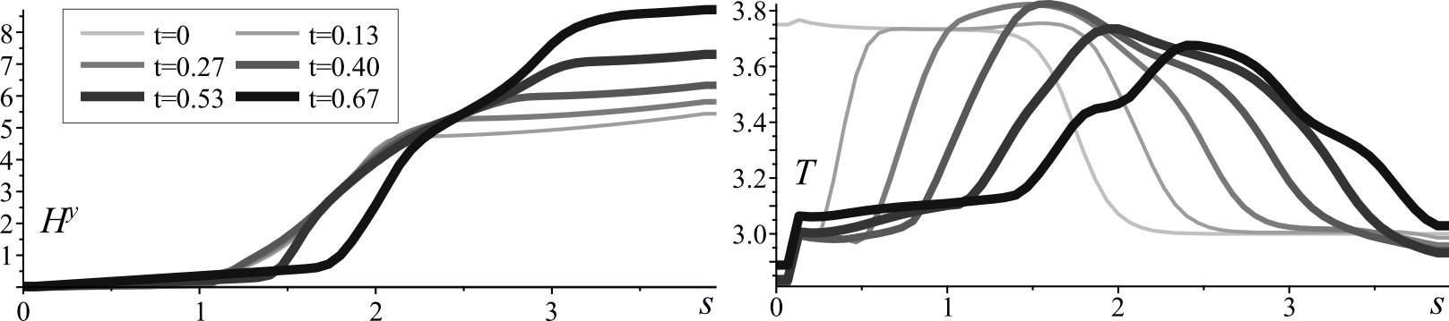
Figure 2: Evolution of the magnetic field $H^{y}$ and the temperature $T$ for the first experiment.

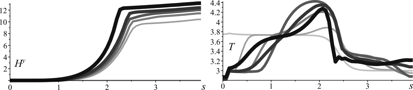
Figure 3: Evolution of the magnetic field $H^{y}$ and the temperature $T$ for the second experiment.

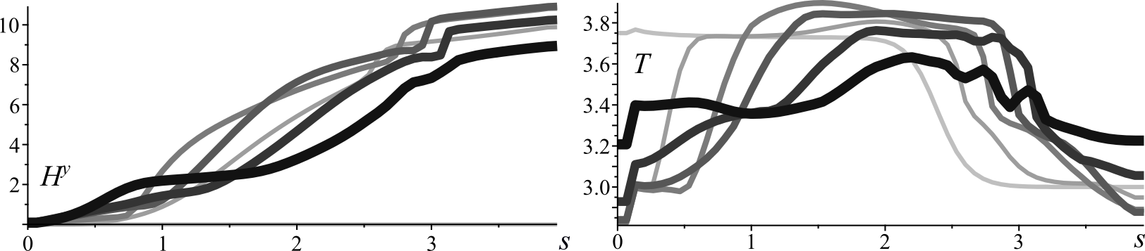
Figure 4: Evolution of the magnetic field $H^{y}$ and the temperature $T$ for the third experiment.

In Figure 5 the trajectories of particles under the action of magnetic fields are shown. The left part (Figure 5, a)–c)) shows $x$-trajectories of particles for three experiments. The right side of the figure shows $y$-trajectories associated with the transverse velocity component $v$. Figure 5, d) corresponds to the first and second experiments where $v$ has a constant value and $H^{0}=0$. Figure 5, e) and Figure 5, f) correspond to the third experiment at $H^{0}>0$ and $H^{0}<0$ where under the action of the longitudinal magnetic field the transverse velocity component increases or slows down accordingly. Notice that the choice of sign of the value $H^{0}$ otherwise does not affect the results of the third experiment.

Figure 5: a), b) and c) show $x$-trajectories for the experiments 1, 2 and 3; d) $y$-trajectories for $H^{0}=0$; e) $y$-trajectories for $H^{0}>0$; f) $y$-trajectories for $H^{0}<0$.

In Figures 6–8 the finite-difference conservation laws of energy, magnetic flux (along the $y$ axis), momentum and center-of-mass motion (along the $x$ axis) are given for the selected moment of time, when the interaction of magnetic fields and the plasma bunch is already quite intense. The results are provided only for the third experiment, since in other cases the control of conservation laws gives similar results. The accurate enough preservation of the conservation laws on solutions is due to the conservativeness of scheme (31).

Figure 6: Conservation laws of energy (solid line) and $y$-flux (dashed line) at $t=0.64$.

Figure 7: Conservation law of $x$-momentum at $t=0.64$.

Figure 8: Conservation law of center-of-mass along axis $x$ at $t=0.64$.

5 Conclusion

Finite-difference schemes for MHD equations in the case of plane one-dimensional flows are considered. The Samarsky–Popov classical scheme for the case of finite conductivity is taken as a starting point. Symmetries and conservation laws of this scheme are investigated. It is shown that the scheme admits the same symmetries as the original differential model. It also has difference analogues of the conservation laws of the original model. In addition to the conservation laws previously known for the scheme, new conservation laws are given, which are obtained on the basis of the group classification recently carried out in Dorodnitsyn et al. (2022).

The classical Samarskiy–Popov scheme is generalized to the case of arbitrary vectors of electric and magnetic fields, as well as to the case of infinite conductivity. In the case of finite conductivity the scheme possesses difference analogues of all differential local conservation laws obtained in Dorodnitsyn et al. (2022), some of which were not previously known. In the case of infinite conductivity, straightforward generalization of the scheme leads to a scheme that does not preserve angular momentum. The proposed modification makes it possible to obtain an invariant scheme that also possesses the conservation law of angular momentum. In addition, it is shown how to approximate the equation of state for a polytropic gas to preserve the entropy along the pathlines on the extended stencil for two time layers.

A numerical implementation of the generalized Samarsky-Popov scheme for the case of finite conductivity is performed for the problem of deceleration of a plasma bunch by crossed electromagnetic fields. Various cases of the action of fields on a plasma are considered. Calculations show that the finite-difference conservation laws are preserved on the solutions of the scheme quite accurately.

Conceptualization, V.D.; methodology, V.D. and E.K.; software, E.K.; validation, E.K; investigation, V.D. and E.K.; data curation, E.K.; writing—original draft preparation, V.D. and E.K.; writing—review and editing, V.D. and E.K.; visualization, E.K.; supervision, V.D.; project administration, V.D.; funding acquisition, V.D. All authors have read and agreed to the published version of the manuscript.

This research was supported by Russian Science Foundation Grant No. 18-11-00238 “Hydrodynamics-type equations: symmetries, conservation laws, invariant difference schemes”.

The data presented in this study are available on request from the corresponding author.

References

• Dorodnitsyn et al. (2022) Dorodnitsyn, V.A.; Kaptsov, E.I.; Kozlov, R.V.; Meleshko, S.V.; Mukdasanit, P. Plane one-dimensional MHD flows: Symmetries and conservation laws. International Journal of Non-Linear Mechanics 2022, 140, 103899.
• Gridnev (1968) Gridnev, N. Study of the magnetohydrodynamics equations’ group properties and invariant solutions. Journal of Applied Mechanics and Technical Physics 1968, pp. 103–107. in Russian.
• Dorodnitsyn (1976) Dorodnitsyn, V.A. On invariant solutions of one-dimensional nonstationary magnetohydrodynamics with finite conductivity. Keldysh Institute preprints 1976, 143. in Russian.
• Rogers (1969) Rogers, C. Invariant Transformations in Non-Steady Gasdynamics and Magneto-Gasdynamics. Zeit angew. Math. Phys. 1969, 20, 370–382.
• Ibragimov (1995) Ibragimov, N.H., Ed. CRC Handbook of Lie Group Analysis of Differential Equations; Vol. 2, CRC Press: Boca Raton, 1995.
• Oliveri and M.P. (2005) Oliveri, F.; M.P., S. Exact solutions to the ideal magneto-gas-dynamics equations through Lie group analysis and substitution principles. J. Phys. A: Math. Gen. 2005, 38, 8803–8820.
• Picard (2008) Picard, P. Some exact solutions of the ideal MHD equations through symmetry reduction. J. Math. Anal. Appl. 2008, 337, 360–385.
• Golovin (2019) Golovin, S. Regular partially invariant solutions of defect 1 of the equations of ideal magnetohydrodynamics. Journal of Applied Mechanics and Technical Physics 2019, 50, 171–180.
• Golovin (2011) Golovin, S. Natural curvilinear coordinates for ideal MHD equations. Non-stationary flows with constant total pressure. Physics Letters, Section A: General, Atomic and Solid State Physics 2011, 375, 283–290.
• Golovin and Sesma (2019) Golovin, S.; Sesma, L. Exact Solutions of Stationary Equations of Ideal Magnetohydrodynamics in the Natural Coordinate System. Journal of Applied Mechanics and Technical Physics 2019, 60, 234–247.
• Toro (1997) Toro, E.F. Riemann Solvers and Numerical Methods for Fluid Dynamics; Springer-Verlag: Berlin-Heidelberg, 1997.
• Samarskiy and Popov (1970) Samarskiy, A.A.; Popov, Y.P. Completely conservative difference schemes for the equations of magneto-hydrodynamics. U.S.S.R. Comput. Math. Math. Phys. 1970, 10, 233–243.
• Samarskii and Popov (1980) Samarskii, A.A.; Popov, Y.P. Difference methods for solving problems of gas dynamics; Nauka: Moscow, 1980. in Russian.
• Falle et al. (1998) Falle, S.A.E.G.; Komissarov, S.S.; Joarder, P. A multidimensional upwind scheme for magnetohydrodynamics. Monthly Notices of the Royal Astronomical Society 1998, 297, 265–277. doi:\changeurlcolorblack10.1046/j.1365-8711.1998.01506.x.
• Powell et al. (1999) Powell, K.G.; Roe, P.L.; Linde, T.J.; Gombosi, T.I.; De Zeeuw, D.L. A Solution-Adaptive Upwind Scheme for Ideal Magnetohydrodynamics. Journal of Computational Physics 1999, 154, 284–309. doi:\changeurlcolorblack10.1006/jcph.1999.6299.
• Yakovlev et al. (2013) Yakovlev, S.; Xu, L.; Li, F. Locally divergence-free central discontinuous Galerkin methods for ideal MHD equations. Journal of Computational Science 2013, 4, 80–91. Computational Methods for Hyperbolic Problems, doi:\changeurlcolorblack10.1016/j.jocs.2012.05.002.
• Yang et al. (2017) Yang, Y.; Feng, X.S.; Jiang, C.W. A high-order CESE scheme with a new divergence-free method for MHD numerical simulation. Journal of Computational Physics 2017, 349, 561–581. doi:\changeurlcolorblack10.1016/j.jcp.2017.08.019.
• Hirabayashi et al. (2016) Hirabayashi, K.; Hoshino, M.; Amano, T. A new framework for magnetohydrodynamic simulations with anisotropic pressure. Journal of Computational Physics 2016, 327, 851–872. doi:\changeurlcolorblack10.1016/j.jcp.2016.09.064.
• Ryu and Jones (1995) Ryu, D.; Jones, T.W. Numerical Magnetohydrodynamics in Astrophysics: Algorithm and Tests for One-dimensional Flow. ApJL 1995, 442, 228. doi:\changeurlcolorblack10.1086/175437.
• Noether (1918) Noether, E. Invariante Variations problem. Konigliche Gesellschaft der Wissenschaften zu Gottingen, Nachrichten, Mathematisch-Physikalische Klasse Heft 2 1918, pp. 235–257. English translation: Transport Theory and Statist. Phys., 1(3), 1971, 183-207.
• Ibragimov (1985) Ibragimov, N.H. Transformation Groups Applied to Mathematical Physics; Reidel: Boston, 1985.
• Olver (1986) Olver, P.J. Applications of Lie Groups to Differential Equations; Springer: New York, 1986.
• Bluman and Anco (2002) Bluman, G.W.; Anco, S.C. Symmetry and Integration Methods for Differential Equations; Springer: New York, 2002; p. 422.
• Dorodnitsyn (1991) Dorodnitsyn, V.A. Transformation groups in net spaces. Journal of Soviet Mathematics 1991, 55, 1490–1517. doi:\changeurlcolorblack10.1007/BF01097535.
• Dorodnitsyn (1994) Dorodnitsyn, V.A. Finite Difference Models Entirely Inheriting Continuous Symmetry of Original Differential Equations. International Journal of Modern Physics C 1994, 05, 723–734. doi:\changeurlcolorblack10.1142/S0129183194000830.
• Maeda (1985) Maeda, S. Extension of discrete Noether theorem. Math. Japonica 1985, 26, 85–90.
• Maeda (1987) Maeda, S. The similarity method for difference equations. J. Inst. Math. Appl. 1987, 38, 129–134.
• Dorodnitsyn (2011) Dorodnitsyn, V.A. Applications of Lie Groups to Difference Equations; CRC Press: Boca Raton, 2011.
• Dorodnitsyn et al. (2004) Dorodnitsyn, V.A.; Kozlov, R.V.; Winternitz, P. Continuous symmetries of Lagrangians and exact solutions of discrete equations. Journal of Mathematical Physics 2004, 45, 336–359. doi:\changeurlcolorblack10.1063/1.1625418.
• Dorodnitsyn et al. (2003) Dorodnitsyn, V.A.; Kozlov, R.V.; Winternitz, P. Symmetries, Lagrangian Formalism and Integration of Second Order Ordinary Difference Equations. Journal of Nonlinear Mathematical Physics Volume Supplement 2003, 10, 41–56. doi:\changeurlcolorblack10.2991/jnmp.2003.10.s2.4.
• Dorodnitsyn and Kozlov (2009) Dorodnitsyn, V.A.; Kozlov, R.V. First integrals of difference Hamiltonian equations. Journal of Physics A: Mathematical and Theoretical 2009, 42, 454007. doi:\changeurlcolorblack10.1088/1751-8113/42/45/454007.
• Dorodnitsyn and Kozlov (2010) Dorodnitsyn, V.A.; Kozlov, R.V. Invariance and first integrals of continuous and discrete Hamiltonian equations. Journal of Engineering Mathematics 2010, 66, 253–270. doi:\changeurlcolorblack10.1007/s10665-009-9312-0.
• Winternitz et al. (2014) Winternitz, P.; Dorodnitsyn, V.A.; Kaptsov, E.I.; Kozlov, R.V. First integrals of difference equations which do not possess a variational formulation. Doklady Mathematics 2014, 89, 106–109. doi:\changeurlcolorblack10.1134/S1064562414010360.
• Dorodnitsyn et al. (2015) Dorodnitsyn, V.A.; Kaptsov, E.I.; Kozlov, R.V.; Winternitz, P. The adjoint equation method for constructing first integrals of difference equations. Journal of Physics A: Mathematical and Theoretical 2015, 48, 055202. doi:\changeurlcolorblack10.1088/1751-8113/48/5/055202.
• Bourlioux et al. (2006) Bourlioux, A.; Cyr-Gagnon, C.; Winternitz, P. Difference schemes with point symmetries and their numerical tests. Journal of Physics A: Mathematical and General 2006, 39, 6877–6896. doi:\changeurlcolorblack10.1088/0305-4470/39/22/006.
• Bourlioux et al. (2007) Bourlioux, A.; Rebelo, R.; Winternitz, P. Symmetry Preserving Discretization of $SL(2,\mathbb{R})$ Invariant Equations. Journal of Nonlinear Mathematical Physics 2007, 15. doi:\changeurlcolorblack10.2991/jnmp.2008.15.s3.35.
• Cheviakov et al. (2020) Cheviakov, A.F.; Dorodnitsyn, V.A.; Kaptsov, E.I. Invariant conservation law-preserving discretizations of linear and nonlinear wave equations. Journal of Mathematical Physics 2020, 61, 081504. doi:\changeurlcolorblack10.1063/5.0004372.
• Dorodnitsyn and Kaptsov (2020) Dorodnitsyn, V.A.; Kaptsov, E.I. Shallow water equations in Lagrangian coordinates: Symmetries, conservation laws and its preservation in difference models. Commun. Nonlinear. Sci. Numer. Simulat. 2020, 89, 105343. doi:\changeurlcolorblack10.1016/j.cnsns.2020.105343.
• Dorodnitsyn et al. (2020) Dorodnitsyn, V.A.; Kaptsov, E.I.; Meleshko, S.V. Symmetries, conservation laws, invariant solutions and difference schemes of the one-dimensional Green-Naghdi equations. Journal of Nonlinear Mathematical Physics 2020. Submitted.
• Dorodnitsyn and Kaptsov (2021) Dorodnitsyn, V.A.; Kaptsov, E.I. Discrete shallow water equations preserving symmetries and conservation laws. Journal of Mathematical Physics 2021, 62, 083508. doi:\changeurlcolorblack10.1063/5.0031936.
• Kaptsov et al. (2021) Kaptsov, E.I.; Dorodnitsyn, V.A.; Meleshko, S.V. Conservative invariant finite-difference schemes for the modified shallow water equations in Lagrangian coordinates. Studies in Applied Mathematics 2021. Submitted.
• Dorodnitsyn et al. (2019) Dorodnitsyn, V.A.; Kozlov, R.; Meleshko, S.V. One-dimensional gas dynamics equations of a polytropic gas in Lagrangian coordinates: Symmetry classification, conservation laws, difference schemes. Commun. Nonlinear. Sci. Numer. Simulat. 2019, 74, 201–218. doi:\changeurlcolorblack10.1016/j.cnsns.2019.03.009.
• Kozlov (2019) Kozlov, R. Conservative difference schemes for one-dimensional flows of polytropic gas. Commun. Nonlinear. Sci. Numer. Simulat. 2019, 78, 104864. doi:\changeurlcolorblack10.1016/j.cnsns.2019.104864.
• Dorodnitsyn et al. (2021) Dorodnitsyn, V.A.; Kozlov, R.V.; Meleshko, S.V. One-dimensional flows of a polytropic gas: Lie group classification, conservation laws, invariant and conservative difference schemes. In Symmetries and Applications of Differential Equations: In Memory of Nail H. Ibragimov (1939-2018); Albert, C.J.L.; Gazizov, R.K., Eds.; Nonlinear Physical Science, Springer Verlag, Singapore, 2021.
• Rojdestvenskiy and Yanenko (1968) Rojdestvenskiy, B.L.; Yanenko, N.N. Systems of quasilinear equations and their applications to gas dynamics; Nauka: Moscow, 1968. in Russian.
• Kulikovskiy and Lyubimov (1965) Kulikovskiy, A.G.; Lyubimov, G.A. Magnetohydrodynamics; International series in physics, Reading, Mass.: Addison-Wesley, 1965.
• Danilova et al. (1973) Danilova, G. V. Dorodnitsyn, V.A.; Kurdyumov, S.P.; Popov, Y.P.; Smarskiy, A.A.; Tsaryova, L.S. Interaction of a plasma clot with a magnetic field in a railgun channel. Keldysh Institute preprints 1973, 62. in Russian.
• Degtyarev and Favorskii (1968) Degtyarev, L.M.; Favorskii, A.P. A flow variant of the sweep method. USSR Computational Mathematics and Mathematical Physics 1968, 8, 252–261. doi:\changeurlcolorblack10.1016/0041-5553(68)90079-7.