A Synergy of Institutional Incentives and Networked Structures in Evolutionary Game Dynamics of Multi-agent Systems

Abstract

Understanding the emergence of prosocial behaviours (e.g., cooperation and trust) among self-interested agents is an important problem in many disciplines. Network structure and institutional incentives (e.g., punishing antisocial agents) are known to promote prosocial behaviours, when acting in isolation, one mechanism being present at a time. Here we study the interplay between these two mechanisms to see whether they are independent, interfering or synergetic. Using evolutionary game theory, we show that punishing antisocial agents and a regular networked structure not only promote prosocial behaviours among agents playing the trust game, but they also interplay with each other, leading to interference or synergy, depending on the game parameters. Synergy emerges on a wider range of parameters than interference does. In this domain, the combination of incentives and networked structure improves the efficiency of incentives, yielding prosocial behaviours at a lower cost than the incentive does alone. This has a significant implication in the promotion of prosocial behaviours in multi-agent systems.

I Introduction

In a wide range of disciplines, it is a fundamental challenge to understand the emergence and maintenance of prosocial behaviours among self-interested agents [1]–[8]. Evolutionary game theory is widely used to study game dynamics of multi-agent systems in games involving prosociality, as for instance, the prisoner’s dilemma, the public goods game, the labour division, and the trust game [4, 1, 9, 2]. Specifically, the replicator equations are widely used for evolutionary game dynamics of multi-agent systems in well-mixed populations, where more successful behaviours are preferably imitated via social learning [10, 1, 9, 5]. Without any additional mechanism, evolutionary game dynamics drives agents not to behave prosocially and, thus, they end up with a lower payoff than what they would get if they all behave prosocially.

Various mechanisms have been proposed to promote prosocial behaviours such as incentives and network reciprocity [4, 1]. Network reciprocity yields the evolution of prosocial behaviours by self-organised clusters of prosocial agents: the spatial structure constrains agents to interact with and imitate only (immediately) neighbouring agents [4, 11]–[14]. Institutional incentives lead to the evolution of prosocial behaviours as well, by either penalising agents for antisocial behaviours or rewarding for prosocial behaviours [1, 5, 8, 15]. Previous works have often studied these two mechanisms in isolation, missing potential interplays between them. In this paper we move a first step towards filling this gap.

Specifically, we use a variant of the replicator equations for evolutionary game dynamics of agents playing the trust game in a structured population with institutional incentives. We analyse the interplay between these two mechanisms in the domain of regular graphs to see whether a combination of them favour or disfavours the evolution of prosocial behaviours. We also find the optimal level of incentive that maximises the population payoff or social welfare, considering the operating cost of incentives. Most previous works have focused on which incentives promote prosocial behaviours best. Another useful measurement for the success of an incentive would be the payoff at the evolutionarily stable state [16].

We decided to focus on the trust game (TG) that has been widely used to formally study trust and trustworthiness in various disciplines [2, 3], [17]–[20]. The TG is a prototypical game or an abstraction of economic transactions that involve buyer and seller interactions for a product or service. Trusting others and reciprocating trust with trustworthy behaviours are important elements of successful economic and social interactions [17]. In engineering research communities, the concept of trust has also attracted significant interest, ranging from networking to human-machine interaction and artificial intelligence [21] while many problems are cast as buyer-seller scenarios [22], [23].

II Model: The Symmetric Binary Trust Game

We use a variant of the TG [20], which makes it a stronger social dilemma than the conventional TG [2], [17]. In our variant of the TG, there are two agents, an investor and a trustee. The investor first decides whether to invest in the trustee or not. If the investor does not invest, then both agents receive a payoff of 0. If the investor invests, then the trustee decides whether to behave trustworthily or untrustworthily. If the trustee is trustworthy (i.e., s/he shares the gain stemming from the investment with the investor) both agents receive $r$, where $0<r<1$. If the trustee is untrustworthy (i.e., not sharing it with the investor), the trustee gets $1$ while the investor gets $-1$. Given a trusting investor, the TG is a social dilemma because: (i) the amount of total payoff ($2r$ or $0$) depends on the trustee’s strategy and (ii) the trustee maximises their payoff by being untrustworthy, which yields a higher payoff of 1 to the trustee but a lower total payoff of 0.

The TG in its original form is asymmetric, meaning that an agent exclusively plays either as an investor or as a trustee [20]. We consider a symmetric TG such that given a pair of agents, one plays as an investor and the other as a trustee: the role allocation is randomly determined with equal probability of 1/2. As an investor, one either invests in a trustee or not. As a trustee, one either acts trustworthily or untrustworthily. Hence, there are 4 strategies that an agent can take $\{IT,IU,NT,NU\}$, where $I$ and $N$ respectively denote ‘invest’ and ‘not invest’, while $T$ and $U$ respectively denote ‘trustworthy’ and ‘untrustworthy’. The payoff matrix of the symmetric TG is given (up to the factor 1/2, which we hereafter omit) by

$$\Pi=\bordermatrix{&IT&IU&NT&NU\cr IT&2r&-1+r&r&-1\cr IU&r+1&0&r&-1\cr NT&r&r&0&0\cr NU&1&1&0&0},$$ (1)

where the elements denote the payoffs that an agent adopting the strategies in the rows acquires when interacting with an agent adopting the strategies in the columns. For instance, the payoff of an agent playing $IT$ with an agent playing $IU$ is $-1+r$.

II-A Incentives

To promote prosocial behaviours (i.e., $I$ and $T$), an institutional incentive scheme lowers the payoff of an agent who acts untrustworthily as a trustee towards an investing investor. The payoff matrix due to the penalty is given by

$$P=\bordermatrix{&IT&IU&NT&NU\cr IT&0&0&0&0\cr IU&-p&-p&0&0\cr NT&0&0&0&0\cr NU&-p&-p&0&0},$$ (2)

where $p\geq 0$ is the expected fine. We assume that each agent pays a tax $f\geq 0$ to maintain the incentive-providing institution. The payoff matrix due to the tax is given by $F=-fJ_{4}$, where $J_{4}$ is a 4$\times$4 matrix with every element being 1. Hence, the net payoff matrix $A$ is given by

$$A=\Pi+P+F.$$ (3)

II-B Evolutionary Game Dynamics

We assume a large population of agents that play the game specified by the payoff matrix $A=[a_{ij}]$ and update their strategies by payoff-led social learning. For instance, an agent can occasionally compare its payoff with that of another agent randomly selected in the population, and imitate the strategy of that player if it has a higher payoff. Assuming that the probability for the imitation is proportional to the payoff difference, the evolution of the frequencies of the strategies in a well-mixed population is given by the replicator equations

$$\dot{x}_{i}=x_{i}\left(\pi_{i}-\bar{\pi}\right)=x_{i}\left(\sum_{j=1}^{4}x_{j}a_{ij}-\sum_{l,j=1}^{4}x_{l}x_{j}a_{lj}\right),$$ (4)

where the dot denotes the time derivative, $x_{i}$ the frequency of the $i$-th strategy, with $i\in\{1,2,3,4\}$, $\mathbf{x}=\left(x_{1},x_{2},x_{3},x_{4}\right)=\left(x_{\text{\tiny IT}},x_{\text{\tiny IU}},x_{\text{\tiny NT}},x_{\text{\tiny NU}}\right)$, $\pi_{i}$ the expected payoff for the $i$-th strategy, and $\bar{\pi}$ the population-mean payoff. The state space is represented by the 3-simplex $\{(x_{1},x_{2},x_{3},x_{4}):x_{1},x_{2},x_{3},x_{4}\geq 0,x_{1}+x_{2}+x_{3}+x_{4}=1\}$. The replicator dynamics of Eq. (4) in a well-mixed population leads to a mixture of $NT$ and $NU$ (equivalent to that of Fig. 1a).

II-B1 Evolutionary Game Dynamics on Graphs

For analytical tractability, we assume that the network structure is specified by a random regular graph with node degree $k\geq 3$, where the agents occupy the nodes of the graph. The game interaction and strategy imitation take place only between neighbouring agents. Using the pair approximation method originally formulated for an infinitely large Caily tree that is well approximated by a large (random) regular graph [24], it is shown that the replicator equations on a regular graph are formally equivalent to those in a well-mixed population with a transformed payoff matrix [13]. Specifically, for the social learning, the replicator dynamics on a graph of node degree $k$ with the payoff matrix $A=[a_{ij}]$ is equivalent to that on a well-mixed population with a payoff matrix $C=[c_{ij}]=[a_{ij}+b_{ij}]$, where

$$b_{ij}=\frac{(k+3)a_{ii}+3a_{ij}-3a_{ji}-(k+3)a_{jj}}{(k+3)(k-2)}.$$ (5)

Thus, the replicator equations on a graph are given by

$$\dot{x}_{i}=x_{i}\left(\sum_{j=1}^{4}x_{j}\left(a_{ij}+b_{ij}\right)-\sum_{l,j=1}^{4}x_{l}x_{j}\left(a_{lj}+b_{lj}\right)\right).$$ (6)

Due to the condition $\sum_{i=1}^{4}x_{i}=1$, there are only three independent variables. Without loss of generality, we take $x_{1}$, $x_{2}$ and $x_{3}$ as independent variables.

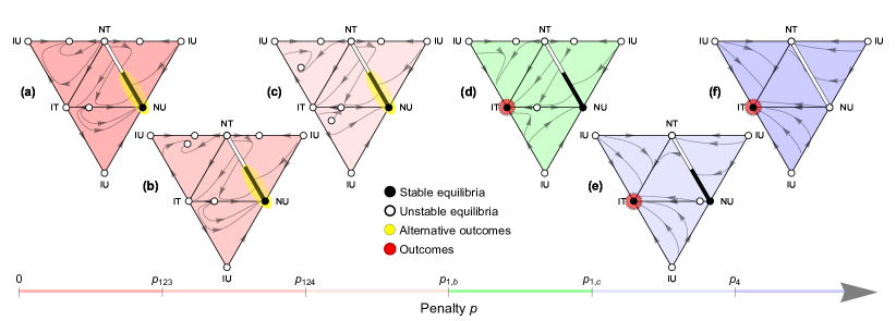
Figure 1: The effect of punishment and networked structure (i.e. a random regular graph) on the evolutionary dynamics of the TG in terms of penalty size $p$. The triangles are the boundaries of a 3-simplex representing the state space. If the penalty is small $p<p_{1,b}$, the population state spends most of the time on the stable part of the line of equilibria $NT$–$NU$ (a) to (c). If $p\geq p_{1,b}$, the population state converges to the $IT$ vertex, i.e., full trust and trustworthiness (d) to (f). (a) For $p<p_{123}$, equilibria appear only on the vertices and edges. (b) For $p_{123}<p<p_{124}$, as $p$ crosses $p_{123}$, the equilibrium in the $IT$–$IU$–$NT$ face emerges from the equilibrium on the $IU$–$NT$ edge. Although the equilibrium in the face has two negative (real parts of) eigenvalues, it is unstable since the remaining eigenvalue is positive. (c) For $p_{124}<p<p_{1,b}$, as $p$ crosses $p_{124}$, the equilibrium in the $IT$–$IU$–$NU$ face emerges from the equilibrium on the $IT$–$NU$ edge. (d) For $p_{1,b}<p<p_{1,c}$, as $p$ crosses $p_{1,b}$, the equilibria in the faces exit the simplex through the $IT$–$IU$ edge and the $IT$ vertex is globally asymptotically stable: from any initial conditions, trajectories converge to $IT$. Even a population state initially on the stable part of the line of equilibria eventually converges to $IT$. The state fluctuates along the line by neutral drift due to random perturbations. Once it has reached the unstable part of the line, an arbitrary small random perturbation can drive it to $IT$. (e) For $p_{1,c}<p<p_{4}$, as $p$ crosses the value $p_{1,c}$, which would be required for the evolution of $IT$ in a well-mixed population, the equilibrium on the $IU$–$NT$ edge moves toward the $NT$ vertex. As $p$ increases and crosses $p_{23}$, the equilibrium merges with the $NT$ vertex. As $p$ further increases, the equilibrium on the $IT$–$NU$ edge moves toward the $NU$ vertex and the stable part of the line of equilibria shrinks. (f) For $p_{4}<p$, as $p$ crosses $p_{4}$, the equilibrium on the $IT$–$NU$ edge merges with the $NU$ vertex and the whole line of equilibria becomes unstable as well as the $NU$ vertex. Parameters: $r=0.6,k=10$, $p/p_{1,c}=p/(1-r)=$ 0.2 (a), 0.4 (b), 0.6 (c), 0.7 (d), 12 (e), and 80 (f).

III Equilibria and stability

To analyse the dynamical system of Eq.(6), we find all equilibria by solving zero states of it, $\dot{x}_{1}=\dot{x}_{2}=\dot{x}_{3}=0$. The stability of an equilibrium is analysed with the signs of eigenvalues of the Jacobian matrix $M$ at the equilibrium, where

$$M=\left(\begin{array}[]{ccc}\frac{\partial\dot{x}_{1}}{\partial x_{1}}&\frac{\partial\dot{x}_{1}}{\partial x_{2}}&\frac{\partial\dot{x}_{1}}{\partial x_{3}}\\ \frac{\partial\dot{x}_{2}}{\partial x_{1}}&\frac{\partial\dot{x}_{2}}{\partial x_{2}}&\frac{\partial\dot{x}_{2}}{\partial x_{3}}\\ \frac{\partial\dot{x}_{3}}{\partial x_{1}}&\frac{\partial\dot{x}_{3}}{\partial x_{2}}&\frac{\partial\dot{x}_{3}}{\partial x_{3}}\end{array}\right).$$ (7)

III-A 1-Morphic Equilibria at the Vertices

III-A1 $x_{\text{\tiny IU}}=x_{\text{\tiny NT}}=x_{\text{\tiny NU}}=0$

The equilibrium $IT$ at the vertex $\left(x_{1},x_{2},x_{3},x_{4}\right)=\left(x_{\text{\tiny IT}},x_{\text{\tiny IU}},x_{\text{\tiny NT}},x_{\text{\tiny NU}}\right)=(1,0,0,0)$ corresponds to a homogeneous state of the population, where all the agents use the same strategy $IT$. The equilibrium $IT$ can be asymptotically stable: trajectories starting close enough to the equilibrium not only remain close enough but also eventually converge to it. The Jacobian $M=[m_{ij}]$ at the equilibrium $IT$ is given by $m_{11}=\frac{-2(k+3)r-3p+6}{k^{2}+k-6}-p-2r+1,m_{12}=\frac{p}{k-2}-r,m_{13}=\frac{3(p+2r)-k(k+1)(p+r-1)}{k^{2}+k-6}$, $m_{22}=-\frac{k(k(p+r-1)+2p+3r-1)}{k^{2}+k-6}$, $m_{33}=\frac{kr}{2-k}$, $m_{21}=m_{23}=m_{31}=m_{32}=0$. $M$ has the three eigenvalues $\lambda_{1,a}=-\frac{kr}{k-2},\lambda_{1,b}=\frac{-k(k+1)(p-1)-2k(k+2)r+3(p+2r)}{k^{2}+k-6}$ and $\lambda_{1,c}=-\frac{k(k(p+r-1)+2p+3r-1)}{k^{2}+k-6}$. If and only if all the eigenvalues are negative, the equilibrium is asymptotically stable. This condition is satisfied in the following three cases. Case $r<\frac{4}{11}$: $\left(k<k_{1,a}\land p>p_{1,a}\right)\lor\left(k>k_{1,a}\land p>p_{1,b}\right)\implies\lambda_{1,a},\lambda_{1,b},\lambda_{1,c}<0$, where $k_{1,a}=\frac{1}{2}\sqrt{\frac{5r^{2}+2r+1}{r^{2}}}+\frac{1-r}{2r}$, $p_{1,a}=\frac{-2k^{2}r+k^{2}-4kr+k+6r}{k^{2}+k-3}$, $p_{1,b}=\frac{k(1-r)-3r+1}{k+2}$, $\land$ and $\lor$ denote logical ‘AND’ and ‘OR’, respectively. Case $\frac{4}{11}\leq r\leq\frac{2}{3}$ : $p>p_{1,b}$ (Fig. 1d). Case $\frac{2}{3}<r$: $\left(k<k_{1,b}\right)\lor\left(k>k_{1,b}\land p>p_{1,b}\right)$, where $k_{1,b}=\frac{3r-1}{1-r}$. As $k\rightarrow\infty$ and, consequently, $p_{1,b}\rightarrow p_{1,c}=1-r$, we recover a well-mixed population, where $IT$ is asymptotically stable for $p>p_{1,c}$. Since $p_{1,b}<p_{1,c}$, in this context punishment promote the prosocial strategy $IT$ in structured populations more efficiently than it does in a well-mixed population. If any of the eigenvalues is positive, $IT$ is unstable.

III-A2 $x_{\text{\tiny IT}}=x_{\text{\tiny NT}}=x_{\text{\tiny NU}}=0$

The equilibrium $IU=(0,1,0,0)$ is unstable since one of the eigenvalues is positive, $\lambda_{2,a}=\frac{(k-1)p}{k-2}+r>0$ (Fig. 1a).

III-A3 $x_{\text{\tiny IT}}=x_{\text{\tiny IU}}=x_{\text{\tiny NU}}=0$

The equilibrium $NT=(0,0,1,0)$ is unstable since one of the eigenvalues is positive, $\lambda_{3,a}=\frac{kr}{k-2}>0$ (Fig. 1a).

III-A4 $x_{\text{\tiny IT}}=x_{\text{\tiny IU}}=x_{\text{\tiny NT}}=0$

The equilibrium $NU=(0,0,0,1)$ can be stable. It has the eigenvalues $\lambda_{4,a}=0,\lambda_{4,b}=-\frac{k(k+p+1)}{k^{2}+k-6}<0$ and $\lambda_{4,c}=\frac{3(p+2r)-k(k-2r+1)}{k^{2}+k-6}$. Since one of the eigenvalues is 0, $NU$ is not asymptotically stable. However, it can be (Lyapunov) stable if none of the eigenvalues is positive: trajectories starting close enough to the equilibrium remain close enough to it. We have $p\leq p_{4}\implies\lambda_{4,c}\leq 0\Longleftrightarrow$ a stable equilibrium, where $p_{4}=\frac{1}{3}\left(k^{2}-2kr+k-6r\right)$ (Fig. 1a). We have $p>p_{4}\implies\lambda_{4,c}>0\Longleftrightarrow$ a unstable equilibrium (Fig. 1f).

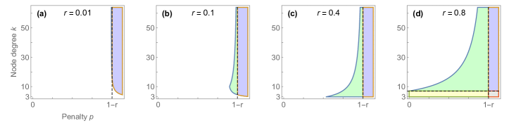
Figure 2: Parameter ranges for the evolution of full trust and trustworthiness. The shaded regions are the ranges of $(p,k)$ where the equilibrium $IT$ is globally asymptotically stable. The dashed vertical line indicates $p=p_{1,c}=1-r$: $p>1-r$ would make $IT$ globally asymptotically stable if there is no networked structure (i.e., $k\rightarrow\infty$ or a well-mixed population). The dashed horizontal line indicates $k=k_{1,b}=(3r-1)/(1-r)$: for $r>2/3$, $k<k_{1,b}$ makes $IT$ globally asymptotically stable even with no incentive in a structured population. Blue: incentive alone ($p>1-r$) would make $IT$ globally asymptotically stable in a well-mixed population and the interplay with networked structure does not make it unstable. Yellow: networked structure alone ($k<k_{1,b}$) would make $IT$ stable and the interplay with incentives does not make it unstable. The region in grey is the intersection of those in blue and yellow. Green: synergy between incentives and networked structure makes $IT$ globally asymptotically stable in spite of $p<1-r$ and $k>k_{1,b}$, each of which would make $IT$ unstable if acting alone. (a) For low $r$, there is little synergy between the incentive and the networked structure. Instead, interference between them can occur for low $k$, where $IT$ is unstable even for large penalty $p>1-r$. (b) to (d) As $r$ increases, synergy emerges and its range expands, whereas interference recedes. (d) As $r$ crosses 2/3, not only the range for synergy further expands but also networked structure can fully induce network reciprocity for $k<k_{1,b}$, making $IT$ globally asymptotically stable even at $p=0$.

III-B 2-Morphic Equilibria on the Edges

III-B1 $x_{\text{\tiny IU}}=x_{\text{\tiny NT}}=0$

The equilibria on the $IT$–$NU$ edge is unstable. It can be found by solving $\pi_{\text{\tiny IT}}(x_{\text{\tiny IT,14}},0,0,1-x_{\text{\tiny IT,14}})=\pi_{\text{\tiny NU}}(x_{\text{\tiny IT,14}},0,0,1-x_{\text{\tiny IT,14}})$, which yields $\mathbf{x}_{\text{\tiny IT--NU}}^{*}=\mathbf{x}_{14}^{*}=\left(x_{\text{\tiny IT,14}}^{*},0,0,1-x_{\text{\tiny IT,14}}^{*}\right)$, where $x_{\text{\tiny IT,14}}^{*}=\frac{k^{2}-2(k+3)r+k-3p}{\left(k^{2}+k-6\right)(p+2r)}$. The condition for the existence of an equilibrium (i.e., $0<x_{\text{\tiny IT,14}}^{*}<1$) is satisfied in the following cases. Case $r\leq\frac{1}{8}\left(2+\sqrt{3}\right):$ $p_{1,a}<p<p_{4}$. Case $\frac{1}{8}\left(2+\sqrt{3}\right)<r<\frac{1}{2}:$ $k\leq k_{14,a}\land p_{1,a}<p<p_{4}$, $k_{14,a}<k<k_{14,b}\land p<p_{4}$, $k=k_{14,b}\land 0<p<p_{4}$, $k>k_{14,b}\land p_{1,a}<p<p_{4}$, where $k_{14,a}=\frac{4r-1-\sqrt{64r^{2}-32r+1}}{2(1-2r)}$, $k_{14,b}=\frac{4r-1+\sqrt{64r^{2}-32r+1}}{2(1-2r)}$. Case $r=\frac{1}{2}$: $k=3\land 0<p<2$, $k\geq 4\land p<\frac{1}{3}\left(k^{2}-3\right)$. Case $\frac{1}{2}<r$: $p<p_{4}$ (Fig. 1a). The equilibrium is unstable since one of the eigenvalues is positive: $\lambda_{14,a}=x_{\text{\tiny IT,14}}^{*}\left(1-x_{\text{\tiny IT,14}}^{*}\right)(p+2r)>0$.

III-B2 $x_{\text{\tiny IT}}=x_{\text{\tiny NU}}=0$

The equilibrium $\mathbf{x}^{*}_{\text{\tiny IU--NT}}=\mathbf{x}^{*}_{23}=\left(0,x_{\text{\tiny IU,23}}^{*},1-x_{\text{\tiny IU,23}}^{*},0\right)$ on the $IU$–$NT$ edge is unstable, where $x_{\text{\tiny IU,23}}^{*}=\frac{1}{2}-\frac{kp}{2(k-2)(p+2r)}$. The condition for the existence of an equilibrium (i.e., $0<x_{\text{\tiny IU,23}}^{*}<1$) is $p<(k-2)r$ (Fig. 1a). Since one of the eigenvalues is negative, $\lambda_{23,a}=-x_{\text{\tiny IU,23}}^{*}(1-x_{\text{\tiny IU,23}}^{*})(p+2r)<0$, the signs of the remaining two eigenvalues determine the stability of the equilibrium. The sum of the remaining eigenvalues is $\lambda_{23,b}+\lambda_{23,c}=\text{Tr}-\lambda_{23,a}=\frac{(p+2r)}{(k-2)}>0$, where Tr is the trace of the Jacobian matrix. The equilibrium is unstable since at least one of the two eigenvalues is positive.

III-B3 $x_{\text{\tiny IT}}=x_{\text{\tiny IU}}=0$

The $NT$–$NU$ edge is a line of equilibria, a part of which can be stable. $\pi_{\text{\tiny NT}}(0,0,1-x_{\text{\tiny NU}},x_{\text{\tiny NU}})=\pi_{\text{\tiny NU}}(0,0,1-x_{\text{\tiny NU}},x_{\text{\tiny NU}})=0$ holds for all $0<x_{\text{\tiny NU}}<1$. The eigenvalues at an equilibrium $(0,0,1-x_{\text{\tiny NU}},x_{\text{\tiny NU}})$ are $\lambda_{34,a}=0,\lambda_{34,b}=-\frac{\left(k^{2}+k-6\right)r(x_{\text{\tiny NU}}-1)+p(k-3x_{\text{\tiny NU}}+3)+k(k+1)x_{\text{\tiny NU}}}{k^{2}+k-6}$ and $\lambda_{34,c}=\frac{-k(k+1)(r+1)x_{\text{\tiny NU}}+k(k+3)r+3x_{\text{\tiny NU}}(p+2r)}{k^{2}+k-6}$. Note that $\lambda_{34,b}<\lambda_{34,c}$. Although the equilibrium cannot be asymptotically stable due to $\lambda_{34,a}=0$, it is stable if and only if $\lambda_{34,b}<0$ and $\lambda_{34,c}\leq 0$, which can be satisfied on a part of the line of equilibria as follows. For $p<p_{4}$, $(0,0,1-x_{\text{\tiny NU}},x_{\text{\tiny NU}})$ is stable with $x_{\text{\tiny NU}}\geq x_{\text{\tiny NU,34}}^{*}$ and unstable with $x_{\text{\tiny NU}}<x_{\text{\tiny NU,34}}^{*}$, where $x_{\text{\tiny NU,34}}^{*}=\frac{k^{2}r+3kr}{k^{2}r+k^{2}+kr+k-3p-6r}$. For $p>p_{4}$, the whole line of equilibria $(0,0,1-x_{\text{\tiny NU}},x_{\text{\tiny NU}})$ is unstable.

III-B4 $x_{\text{\tiny IU}}=x_{\text{\tiny NU}}=0$

There is no equilibrium on the $IT$–$NT$ edge since $\pi_{\text{\tiny IT}}\left(x_{\text{\tiny IT}},0,1-x_{\text{\tiny IT}},0\right)-\pi_{\text{\tiny NT}}(x_{\text{\tiny IT}},0,1-x_{\text{\tiny IT}},0)=\frac{kr}{k-2}>0$, whereas $\pi_{\text{\tiny IT}}=\pi_{\text{\tiny NT}}$ should hold at an equilibrium.

III-B5 $x_{\text{\tiny IT}}=x_{\text{\tiny NT}}=0$

There is no equilibrium on the $IU$–$NU$ edge since $\pi_{\text{\tiny IU}}(0,x_{\text{\tiny IU}},0,1-x_{\text{\tiny IU}})-\pi_{\text{\tiny NU}}(0,x_{\text{\tiny IU}},0,1-x_{\text{\tiny IU}})=-\frac{x_{\text{\tiny IU}}\left[k(k+1)(p+r-1)-3(p+2r)\right]+k(k+p+1)}{k^{2}+k-6}<0$, where $0<x_{\text{\tiny IU}}<1$.

III-B6 $x_{\text{\tiny NT}}=x_{\text{\tiny NU}}=0$

The $IT$–$IU$ edge is a line of equilibria, which is degenerate. The condition for the equilibria $\pi_{\text{\tiny IT}}(x_{\text{\tiny IT}},1-x_{\text{\tiny IT}},0,0)-\pi_{\text{\tiny IU}}(x_{\text{\tiny IT}},1-x_{\text{\tiny IT}},0,0)=\frac{k\left[p(k+2)+(k+3)r-k-1\right]}{k^{2}+k-6}=0$ is satisfied for the whole edge at $p=\frac{-(k+3)r+k+1}{k+2}\land r\leq\frac{2}{3}$. Holding only at a particular value of $p$ for given $r\leq\frac{2}{3}$ and $k$, however, the line of equilibria is degenerate or structurally unstable, because an arbitrarily small perturbation in $p$ leads the line of equilibria to disappear.

III-C 3-Morphic Equilibria on the Faces

III-C1 $x_{\text{\tiny NU}}=0$

The equilibrium $\mathbf{x}_{\text{\tiny IT--IU--NT}}^{*}=\mathbf{x}_{123}^{*}=\left(1-x_{\text{\tiny IU,123}}^{*}-x_{\text{\tiny NT,123}}^{*},x_{\text{\tiny IU,123}}^{*},x_{\text{\tiny NT,123}}^{*},0\right)$ on the $IT$–$IU$–$NT$ face is unstable, where $x_{\text{\tiny IU,123}}^{*}=\frac{k(k+3)r}{k(k+1)(r+1)-3(p+2r)}$ and $x_{\text{\tiny NT,123}}^{*}=\frac{k(k(p+r-1)+2p+3r-1)}{k(k+1)(p+r-1)-3(p+2r)}$. The equilibrium is found by solving $\pi_{\text{\tiny IT}}(1-x_{\text{\tiny IU}}-x_{\text{\tiny NT}},x_{\text{\tiny IU}},x_{\text{\tiny NT}},0)=\pi_{\text{\tiny IU}}(1-x_{\text{\tiny IU}}-x_{\text{\tiny NT}},x_{\text{\tiny IU}},x_{\text{\tiny NT}},0)=\pi_{\text{\tiny NT}}(1-x_{\text{\tiny IU}}-x_{\text{\tiny NT}},x_{\text{\tiny IU}},x_{\text{\tiny NT}},0)$. The conditions for existence of the equilibrium (i.e., $0<x_{\text{\tiny IU,123}}^{*},x_{\text{\tiny NT,123}}^{*},1-x_{\text{\tiny IU,123}}^{*}-x_{\text{\tiny NT,123}}^{*}<1$) are satisfied in the following cases. Case $0<r<\frac{2}{5}$: $p_{123}<p<p_{1,b}$, where $p_{123}=\frac{1}{6}(k^{3}r+2k^{2}r+k^{2}-2kr+k-12r)-\frac{1}{6}(k^{6}r^{2}+4k^{5}r^{2}-20k^{3}r^{2}-8k^{2}r^{2}+2k^{5}r+6k^{4}r-12k^{3}r-16k^{2}r+k^{4}+2k^{3}+k^{2})^{1/2}$. Case $\frac{2}{5}<r$: $k_{1,b}<k<k_{123}\land p<p_{1,b}$, $k>k_{123}\land p_{123}<p<p_{1,b}$, where $k_{123}=\frac{1}{2}\sqrt{\frac{r^{2}+14r+1}{(r-1)^{2}}}+\frac{1-5r}{2(r-1)}$. The equilibrium is unstable since one of the eigenvalues is positive, $\lambda_{123,a}=\frac{p+2r}{k-2}>0$ (Fig. 1b).

III-C2 $x_{\text{\tiny NT}}=0$

The equilibrium $\mathbf{x}_{\text{\tiny IT--IU--NU}}^{*}=\mathbf{x}_{\text{124}}^{*}=(x_{\text{\tiny IT,124}}^{*},1-x_{\text{\tiny IT,124}}^{*}-x_{\text{\tiny NU,124}}^{*},0,x_{\text{\tiny NU,124}}^{*})$ on the $IT$–$IU$–$NU$ face is unstable, where $x_{\text{\tiny IT,124}}^{*}=\frac{k(k+p+1)}{k(k+1)(r+1)-3(p+2r)}$ and $x_{\text{\tiny NU,124}}^{*}=\frac{k(k(p+r-1)+2p+3r-1)}{k(k+1)(p+r-1)-3(p+2r)}$. The conditions for existence of the equilibrium (i.e., $0<x_{\text{\tiny IT,124}}^{*},x_{\text{\tiny NU,124}}^{*},1-x_{\text{\tiny IT,124}}^{*}-x_{\text{\tiny NU,124}}^{*}<1$) are satisfied in the following cases. Case $r\leq\frac{4}{11}$: $k>\frac{1}{2}\sqrt{\frac{5r^{2}+2r+1}{r^{2}}}+\frac{1-r}{2r}\land p_{124}<p<p_{1,b}$, where $p_{124}=\frac{1}{2}\frac{36r-k\left((k(2k+5)-15)r+k(k+1)^{2}\right)}{k\left(k^{2}+k-6\right)-9}+\frac{1}{2}\frac{\sqrt{k^{2}(k+3)^{2}\left(\left(k^{2}-4\right)(k+1)^{2}+(17-4(k-1)k)r^{2}-2(k-2)(k+1)r\right)}}{k\left(k^{2}+k-6\right)-9}$. Case $\frac{4}{11}<r\leq\frac{1}{2}\left(\sqrt{17}-3\right)$: $p_{124}<p<p_{1,b}$. Case $\frac{1}{2}\left(\sqrt{17}-3\right)<r<\frac{2}{3}$: $\left(k<k_{124}\land p<p_{1,b}\right)\lor\left(k>k_{124}\land p_{124}<p<p_{1,b}\right)$. Case $\frac{2}{3}\leq r$: $\left(k_{1,b}<k<k_{124}\land p<p_{1,b}\right)\lor(k>k_{124}\land p_{124}<p<p_{1,b})$, where $k_{124}$ is the 2nd root of $0=k^{4}(r-1)+k^{3}\left(2r^{2}+4r-2\right)+k^{2}\left(8r^{2}+3r-1\right)-6kr^{2}-36r^{2}$.

Although the first eigenvalue $\lambda_{124,a}=-\frac{p+2r}{k-2}<0$ is negative, the sum of remaining two eigenvalues is $\lambda_{124,b}+\lambda_{124,c}=\text{Tr}-\lambda_{124,a}=\frac{k^{2}(k+p+1)(p+2r)\left[(k+2)p+k(r-1)+3r-1\right]}{\left[-3p+k(k+1)(r+1)-6r\right]\left[\left(k(1+k)-3\right)p+k(1+k)(r-1)-6r\right]}>0$ and, thus, one of the (real parts of) two eigenvalues is positive. Hence, the equilibrium is unstable (Fig. 1c).

III-C3 $x_{\text{\tiny IU}}=0$

The equilibria on the $IT$–$IU$–$NT$ face are degenerate. A line of equilibria exists only at a particular value of $p=\frac{6r-k(k+1)(r-1)}{k^{2}+k-3}$, given $r$ and $k$.

III-C4 $x_{\text{\tiny IT}}=0$

The equilibria on the $IU$–$NT$–$NU$ face are degenerate for the same reason as above.

III-D No 4-Morphic or Interior Equilibrium

There is no interior equilibrium. For an interior point $(x_{\text{\tiny IT}},x_{\text{\tiny IU}},x_{\text{\tiny NT}},x_{\text{\tiny NU}})$, i.e., $0<x_{\text{\tiny IT}},x_{\text{\tiny IU}},x_{\text{\tiny NT}},x_{\text{\tiny NU}}<1$, we have $\pi_{\text{\tiny NT}}(x_{\text{\tiny IT}},x_{\text{\tiny IU}},x_{\text{\tiny NT}},x_{\text{\tiny NU}})\neq\pi_{\text{\tiny NU}}(x_{\text{\tiny IT}},x_{\text{\tiny IU}},x_{\text{\tiny NT}},x_{\text{\tiny NU}})$ since $\pi_{\text{\tiny NT}}-\pi_{\text{\tiny NU}}=-\frac{(x_{\text{\tiny IT}}+x_{\text{\tiny IU}})(k(k+1)(1-r-p)+3(p+2r))}{(k-2)(k+3)}<0$ for $p\leq 1-r$ and $\pi_{\text{\tiny NT}}-\pi_{\text{\tiny NU}}=[p((k+3)w+(k+3)z)+(k+3)r(2w+2z)+k(x_{\text{\tiny IT}}+x_{\text{\tiny IU}})((p+r-1)k+2p-3r-1)]/[(k-2)(k+3)]>0$ for $p>1-r$. Hence, no interior point satisfies the condition $\pi_{\text{\tiny IT}}=\pi_{\text{\tiny IU}}=\pi_{\text{\tiny NT}}=\pi_{\text{\tiny NU}}$ for an equilibrium.

In general, replicator dynamics of a normal-form or matrix-form game with four strategies can have steady states (e.g., a limit cycle or a chaotic attractor) other than an isolated equilibrium point in the interior state space. Since the dynamical system of Eq. (6) contains no interior equilibrium, however, there exist no steady states in the interior state space, according to Theorem 7.6.1 of the reference [25].

IV Interference and Synergy

Our analysis shows that punishment and random regular graphs interact in a non-trivial way. For low $r$, interference can occur at low node degrees $k$: this prevents the evolution of the prosocial strategy $IT$ even at a high level of penalty $p>p_{1,c}$ that would be sufficient if the evolution were on a well-mixed population (Fig. 2a). As $r$ increases, however, interference recedes whereas synergy emerges and the range of it expands: a combination of even low penalty and weakly networked structure (i.e., large degrees) can lead to the evolution of $IT$, each of which would fail if acting alone (Fig. 2b to 2d). The synergy not only lowers the level of penalty $p=p_{1,b}$ required for the evolution of $IT$ but also yields a higher payoff than penalty alone $p=p_{1,c}$ does in a well-mixed population (Fig. 3).

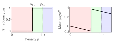
Figure 3: The frequency $x_{\text{\tiny IT}}$ of the prosocial strategy $IT$ and population-mean payoff at the evolutionary stable state in terms of penalty size $p$ in a structured population. While the evolution of $IT$ is maintained for $p\geq p_{1,b}$, the mean payoff is optimal at $p=p_{1,b}$. Parameters: $r=0.6,k=10,f=p$.

We have shown that simple networks are sufficient to yield a substantial interplay with incentives for promoting pro-social behaviours in large multi-agent systems. For future work, impacts of complex networks, stochastic game dynamics, interplays between other mechanisms in TG and other games involving pro-sociality will also be well worth studying.

References

• [1] J. Zhang and M. Cao, “Strategy competition dynamics of multi-agent systems in the framework of evolutionary game theory,” IEEE Transactions on Circuits and Systems II: Express Briefs, vol. 67, no. 1, pp. 152–156, 2020.
• [2] H. Abbass, G. Greenwood, and E. Petraki, “The $n$-player trust game and its replicator dynamics,” IEEE Transactions on Evolutionary Computation, vol. 20, no. 3, pp. 470–474, 2016.
• [3] I. S. Lim, “Stochastic evolutionary dynamics of trust games with asymmetric parameters,” Physical Review E, vol. 102, no. 6, pp. 062 419–, 12 2020.
• [4] M. A. Nowak, “Five rules for the evolution of cooperation,” Science, vol. 314, no. 5805, pp. 1560–1563, 12 2006.
• [5] T. Sasaki, Å. Brännström, U. Dieckmann, and K. Sigmund, “The take-it-or-leave-it option allows small penalties to overcome social dilemmas,” Proceedings of the National Academy of Sciences, vol. 109, no. 4, p. 1165, 01 2012.
• [6] V. Capraro and M. Perc, “Mathematical foundations of moral preferences,” Journal of The Royal Society Interface, vol. 18, no. 175, p. 20200880, 2021.
• [7] M. Perc, J. J. Jordan, D. G. Rand, Z. Wang, S. Boccaletti, and A. Szolnoki, “Statistical physics of human cooperation,” Physics Reports, vol. 687, pp. 1–51, 2017.
• [8] K. Sigmund, H. De Silva, A. Traulsen, and C. Hauert, “Social learning promotes institutions for governing the commons,” Nature, vol. 466, no. 7308, pp. 861–863, 2010.
• [9] C. Zhang, Q. Li, Y. Zhu, and J. Zhang, “Dynamics of task allocation based on game theory in multi-agent systems,” IEEE Transactions on Circuits and Systems II: Express Briefs, vol. 66, no. 6, pp. 1068–1072, 2019.
• [10] P. D. Taylor and L. B. Jonker, “Evolutionary stable strategies and game dynamics,” Mathematical Biosciences, vol. 40, no. 1–2, pp. 145 – 156, 1978.
• [11] H. Ohtsuki, C. Hauert, E. Lieberman, and M. A. Nowak, “A simple rule for the evolution of cooperation on graphs and social networks,” Nature, vol. 441, no. 7092, pp. 502–505, 05 2006.
• [12] M. Chica, R. Chiong, M. Kirley, and H. Ishibuchi, “A networked n-player trust game and its evolutionary dynamics,” IEEE Transactions on Evolutionary Computation, vol. 22, no. 6, pp. 866–878, 2018.
• [13] H. Ohtsuki and M. A. Nowak, “The replicator equation on graphs,” Journal of Theoretical Biology, vol. 243, no. 1, pp. 86–97, 2006.
• [14] J. M. Pacheco, A. Traulsen, and M. A. Nowak, “Coevolution of strategy and structure in complex networks with dynamical linking,” Physical Review Letters, vol. 97, no. 25, pp. 258 103–, 12 2006.
• [15] X. Fang and X. Chen, “Evolutionary dynamics of trust in the n-player trust game with individual reward and punishment,” The European Physical Journal B, vol. 94, no. 9, p. 176, 2021.
• [16] Y. Dong, T. Sasaki, and B. Zhang, “The competitive advantage of institutional reward,” Proceedings of the Royal Society B: Biological Sciences, vol. 286, no. 1899, p. 20190001, 2019.
• [17] N. D. Johnson and A. A. Mislin, “Trust games: A meta-analysis,” Journal of Economic Psychology, vol. 32, no. 5, pp. 865–889, 2011.
• [18] C. Tarnita, “Fairness and trust in structured populations,” Games, vol. 6, no. 3, pp. 214–230, 2015.
• [19] A. Kumar, V. Capraro, and M. Perc, “The evolution of trust and trustworthiness,” Journal of The Royal Society Interface, vol. 17, no. 169, p. 20200491, 2020.
• [20] N. Masuda and M. Nakamura, “Coevolution of trustful buyers and cooperative sellers in the trust game,” PloS one, vol. 7, no. 9, p. e44169, 2012.
• [21] J.-H. Cho, K. Chan, and S. Adali, “A survey on trust modeling,” ACM Computing Surveys, vol. 48, no. 2, pp. 28:1–40, 2015.
• [22] T. Jung, X. Li, W. Huang, Z. Qiao, J. Qian, L. Chen, J. Han, and J. Hou, “Accounttrade: Accountability against dishonest big data buyers and sellers,” IEEE Transactions on Information Forensics and Security, vol. 14, no. 1, pp. 223–234, 2019.
• [23] D. Niyato, E. Hossain, and Z. Han, “Dynamics of multiple-seller and multiple-buyer spectrum trading in cognitive radio networks: A game-theoretic modeling approach,” IEEE Transactions on Mobile Computing, vol. 8, no. 8, pp. 1009–1022, 2009.
• [24] H. Matsuda, N. Ogita, A. Sasaki, and K. Satō, “Statistical mechanics of population: The lattice lotka-volterra model,” Progress of Theoretical Physics, vol. 88, no. 6, pp. 1035–1049, 1992.
• [25] J. Hofbauer and K. Sigmund, Evolutionary Games and Population Dynamics.   Cambridge University Press, 1998.