HTMOT : Hierarchical Topic Modelling Over Time

Abstract

Topic models provide an efficient way of extracting insights from text and supporting decision-making. Recently, novel methods have been proposed to model topic hierarchy or temporality. Modeling temporality provides more precise topics by separating topics that are characterized by similar words but located over distinct time periods. Conversely, modeling hierarchy provides a more detailed view of the content of a corpus by providing topics and sub-topics. However, no models have been proposed to incorporate both hierarchy and temporality which could be beneficial for applications such as environment scanning. Therefore, we propose a novel method to perform Hierarchical Topic Modelling Over Time (HTMOT). We evaluate the performance of our approach on a corpus of news articles using the Word Intrusion task. Results demonstrate that our model produces topics that elegantly combine a hierarchical structure and a temporal aspect. Furthermore, our proposed Gibbs sampling implementation shows competitive performance compared to previous state-of-the-art methods.

1 Introduction

In NLP, over the years, several methods for extracting themes (or topics) from a corpus have been proposed (Alghamdi and Alfalqi, 2015; Barde and Bainwad, 2017). These topic models have been applied to various tasks, including document summarization (Yang et al., 2015), environment scanning (Gregoriades et al., 2021; Kim et al., 2020), understanding employee and customer satisfaction (Korfiatis et al., 2019; Bastani et al., 2019) among others.

The seminal LDA algorithm (Blei et al., 2003) leads the way for the study of topic models. However, LDA requires the user to specify a predefined number of topics to be extracted. Furthermore, LDA generates a flat topic structure with no hierarchical or temporal information.

Recently, hierarchical topic models have been proposed (Paisley et al., 2015; Blei et al., 2004). Such models enable the extraction of topics and sub-topics organised in a tree-like hierarchy. Additionally, these models dynamically determine the appropriate number of topics and sub-topics during training. These models are particularly useful in applications such as ontology learning (Zhu et al., 2017) and research idea recommendation(Wang et al., 2019).

In parallel, temporal topic models have been proposed (Wang and McCallum, 2006; Nallapati et al., 2007; Song et al., 2008; Blei and Lafferty, 2006). Incorporating temporal information enables the extraction of topics that can describe events or trends occurring in a corpus. They have been used for tracking trends in scientific articles (Hong et al., 2011) and events in social media (Zhou and Chen, 2013).

Intuitively, incorporating temporal and hierarchical information would yield models that encompass the strengths of both. Several applications would benefit from this incorporation such as environment scanning(El Akrouchi et al., 2021). This task is defined as gathering, analyzing and monitoring information that is relevant to an organization to identify future threats and opportunities. Understandably, this task would benefit from having both hierarchical and temporal modelling.

Hierarchical modelling would provide more detailed topics as it extracts topics but also sub-topics which deepens our understanding of a thematic. Conversely, temporal modelling would provide more precise topics describing specific events.

However, to date, no topic model integrating both temporal and hierarchical information have been proposed. The main reason is the difficulty in integrating time and hierarchy. Many temporal topic models have their own structure to represent time, e.g. time trees (Nallapati et al., 2007) or time slices (Song et al., 2008; Blei and Lafferty, 2006). Coupling such temporal structure with a hierarchical structure is extremely challenging. Nonetheless, there is one temporal model (ToT) (Wang and McCallum, 2006) that does not require its own structure. Even in this case, combining time and hierarchy is still difficult for several reasons: Firstly, the beta distribution used to model time in ToT does not have a known conjugate prior. Hence, it is not compatible with stochastic variational inference (SVI) used by previous hierarchical models. Secondly, applying temporality to every topics would split them into various periods. Each of these splits would have similar sub-topics, which would lead to an unnecessary multiplication of topics.

Therefore, as our main contribution, we propose a novel method for Hierarchical Topic Modelling Over Time (HTMOT). By jointly modelling topic hierarchy and temporality, our model offers the advantages of previous methods, which only focused on a single dimension (i.e. temporality or hierarchy). Specifically, we model temporality at the deepest level of the topic tree to extract more precise sub-topics and avoid splitting high level topics. To the best of our knowledge, our model is the first to jointly model topic hierarchy and temporality.

As a secondary contribution, we propose a novel implementation of Gibbs sampling. We use Gibbs sampling as it was found to be suitable to model temporality (Wang and McCallum, 2006) contrary to SVI. However, the original Gibbs sampling implementation is prohibitively slow. Thus, we propose an enhanced implementation based on a novel tree-based data structure, which we call the Infinite Dirichlet Tree. As a result our Gibbs sampling implementation is comparable to SVI in term of speed.

We performed our experiments using a corpus of 62k news articles and evaluated our method using the Word Intrusion task (Chang et al., 2009).

2 Related Work

We now describe previous topic modelling methods most closely related to ours. Table 2 summarize these models as well as their associated datasets. For more comprehensive reviews see Alghamdi and Alfalqi (2015) and Barde and Bainwad (2017).

2.1 Topic Modelling

The seminal LDA (Blei et al., 2003) algorithm remains the most popular topic model. It is at the basis of most subsequent models. At the core of LDA is a Bayesian generative model based on Dirichlet distributions. These are used to model the document-topic and the topic-word distributions. They are learnt and optimized via an inference procedure, which enables topics to be extracted. The main weakness of LDA is that it requires the user to specify a predefined number of topics to be extracted. However, such information is usually not known in advance. Consequently, LDA requires a long model validation step to determine the number of topics.

The subsequent HDP Teh et al. (2006) model uses Dirichlet processes (DPs) to determine the number of topics during training. Using DPs allows us to have an indefinite number of topics contrary to Dirichlet distributions. Otherwise, HDP operates similarly to LDA.

2.2 Hierarchical Topic Modelling

Methods such as LDA and HDP are only capable of extracting a flat topic structure. Hence, new methods have been developed to model topic hierarchies. By extracting topics and sub-topics, we end up with more detailed information about a corpus.

The state-of-the-art for hierarchical topic modelling is nHDP (Paisley et al., 2015). It models topic hierarchy by defining a potentially infinite tree where each node corresponds to a topic. At each branch of the tree, we exactly have the HDP model. The difference is that, when a word is assigned to a topic during training, there is a chance to go deeper in the tree based on a Bernoulli distribution. If we do go deeper, we repeat the HDP algorithm with a sub-corpus made up of the documents and tokens assigned to the selected topic.

Other topic models have been proposed to model hierarchy. hPAM (Mimno et al., 2007) proposes a directed acyclical graph structure instead of a tree to model topic hierarchy. Thus, high level topics can share low level topics. While this provides more precise relationships between topics, it is harder to display and navigate. LSHTM (Pujara and Skomoroch, 2012) recursively applies LDA to the sub-corpus defined by the topics of the previous LDA application. Hence, each new application of LDA provides a new depth to the topic tree. However, it requires a pre-defined set of parameters to define the shape of the final topic tree. Finally, the nCRP (Blei et al., 2004) is the predecessor of nHDP and works similarly. Nevertheless, it does not model the document-topic distribution as in nHDP. Consequently, the extracted documents do not have their own topic tree. Hence, nHDP is more powerful than LSHTM and nCRP(Pujara and Skomoroch, 2012; Blei et al., 2004) while keeping a strict tree structure contrary to hPAM (Mimno et al., 2007).

2.3 Temporal Topic Modelling

Previous works also investigated the temporality of topics. Providing information about when a topic occurred and/or how it evolved. Understanding the temporality of topics is important, especially for environment scanning where events and changes in the environment are important signals.

The ToT (Wang and McCallum, 2006) model is a modified version of LDA which incorporates temporality. Each document/word is associated with a timestamp which are used to fit a beta distribution for each topic. This beta distribution is optimized jointly as the topics are being discovered. The results show topics that are either better localized in time (events with specific dates) or with a clear evolution through time (growth/decline).

Other topic models have been proposed to model temporality. MTT (Nallapati et al., 2007) creates a tree for each topic which provides the ability to understand topics at various time scale. Specifically, deeper nodes correspond to a smaller timescale. DTM (Blei and Lafferty, 2006) slices the corpus by periods. The first slice is processed similarly to LDA and the following slices are processed using the previous one as prior. Finally, DCTM (Song et al., 2008) also slices the corpus in period. However, it uses Gaussian processes and SVD instead of LDA based techniques. The advantage of ToT is that it is non-Markovian and it models time as a continuum. Hence, ToT is the only model which does not require its own structure to model time such as slices or a binary tree. This is important if we are already building a structure for the topic hierarchy.

2.4 Topic Models Evaluation

Various methods have been used in previous studies to evaluate topic models such as perplexity and coherence. However, these methods have been repeatedly demonstrated to be uncorrelated with human judgement (Chang et al., 2009; Hoyle et al., 2021).

The Word Intrusion task is the latest evaluation method devised. For each topic, it involves inserting an intruder word in the topic top word list and then asking annotators to find it (Chang et al., 2009). This intruder is selected at random from a pool of words with low probability in the current topic but high probability in some other topic to avoid rare words. The idea is that in good topics, the annotators would easily find this intruder. With this evaluation method, the final score corresponds to the average classification accuracy made by humans. In Lau et al. (2014) , they have shown that this task can be automated with performance similar to human annotators.

3 HTMOT : Hierarchical Topic Modelling Over Time

We now describe our method for Hierarchical Topic Modelling Over Time (HTMOT). We begin by presenting a new type of data structure at the core of HTMOT (section 3.1). Next, we describe how temporality was incorporated into the hierarchy (section 3.2). Then, we detail our novel implementation of Gibbs sampling (section 3.3). Finally, we denote important differences between HTMOT and its predecessor (section 3.4).

3.1 Counting words using Infinite Dirichlet Trees

Infinite Dirichlet Trees (IDTs) are efficient tree-based data structures we developed. The name refers to the potentially infinite number of topics provided by the Dirichlet Processes, which define how they grow. The role of these trees is to model the topics, their hierarchical dependency and temporality. Hence, these trees are optimized during the training process to serve as the final output of HTMOT.

Each node of an IDT is identified by a finite path in the tree as a sequence of node ids, starting from the root. For example the node "root.A.B" corresponds to a sub-topic of the topic "Root.A". The nodes record word assignments (see figure 1) and the timestamps of those words (associated with the source document). Thus, each node represents a topic and defines a topic-word and a topic-time distribution.

The trees also model the hierarchical distribution of topics. Words are assigned to a final topic and to all ancestors of that topic. Hence, there are two types of word assignments : "through" and "final", respectively for the ancestor topics and final topic. This creates a hierarchical dependency between the nodes and thus a hierarchical distribution.

We use multiple IDTs, one for the corpus and one for each document. All words in the corpus are assigned to nodes of the corpus tree. Similarly, each document has an associated document tree recording each word of that document. Hence, combining all document trees together would yield the corpus tree. For both the corpus and document trees, each node (topic) will be assigned a different number of words. Thus, nodes differ in size which creates a distribution. Hence, the corpus tree defines a corpus-topic distribution and each document tree defines a document-topic distribution.

From the foregoing discussion, we can see that the assignment of words to the different trees defines the topic-word, topic-time, document-topic, corpus-topic and topic-hierarchy distributions. Hence, by simply moving words around in those trees, we can optimize all these distributions jointly. Once optimized, the trees can be used directly as output to view topics, their hierarchy and temporality for the corpus and each document.

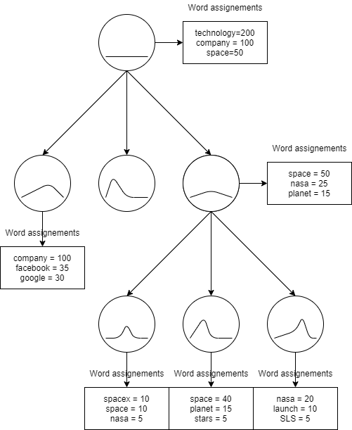
Figure 1: Example of an IDT with word assignments and time distribution (inside nodes).

3.2 Modelling temporality

Temporality is modelled by associating topics with a beta distribution as in ToT (Wang and McCallum, 2006). This allows us to extract topics that describe specific event in time. Mathematically, we separate topics that are lexically similar but located at different periods in time. However, applying temporality to high level topic would split them into various periods. Each of these splits would have similar sub-topics, which would lead to an unnecessary multiplication of topics. Hence, contrary to ToT, we do not apply temporality to all topics but only deep ones. For our experiments, we choose depths of 3 or more. This allows us to extract precise topics about specific events in time at the deeper levels while keeping the high level topics intact.

The parameters of the beta distribution $\rho^{1}_{i}$ and $\rho^{2}_{i}$ are computed for a topic $i$ based on the current timestamps assignments (associated with each word assignment). We used the method of the moment to estimate these parameters :

$$\rho^{1}_{i}=\overline{t_{i}}*(\frac{\overline{t_{i}}*(1-\overline{t_{i}})}{\sigma_{t_{i}}}-1)$$ (1)

$$\rho^{2}_{i}=(1-\overline{t_{i}})*(\frac{\overline{t_{i}}*(1-\overline{t_{i}})}{\sigma_{t_{i}}}-1)$$ (2)

Where $\overline{t_{i}}$ is the empirical average timestamp assigned to topic $i$ and $\sigma_{t_{i}}$ is the empirical variance. These parameters are updated each time a word is assigned or unassigned to topic $i$.

3.3 Training HTMOT using Gibbs sampling

Algorithm 1 Traditional Gibbs sampling

1:procedure ClassicGibbs($corpus$)

2:     for N iterations do

3:         for each $document$ in $corpus$ do

4:              for each $word$ in $document$ do

5:                  Sample word-topic assignment

6:                  Sample topic-word

7:                  Sample document-topic

8:                  Estimate time-topic

9:                  Sample corpus-topic

10:                  Sample hierarchy-topic

11:              end for

12:         end for

13:     end for

14:     Return solution

15:end procedure

Two methods are commonly used for training topic models : Gibbs sampling and Stochastic Variational inference (SVI). Gibbs sampling is asymptotically exact, i.e. it can exactly approximate the target distribution, unlike SVI (Blei et al., 2017). However, classical implementations of Gibbs sampling are prohibitively slow as they require sampling from all distributions (see algorithm 1).

Nevertheless, in the context of topic modelling, we can avoid this issue (Xiao and Stibor, 2010) and greatly speed up the process. Specifically, it is possible to only draw from the word-topic assignment distribution. This requires the construction of a data structure tailored to the model to implicitly represent the other distributions. This is the role played by our Infinite Dirichlet Trees.

As stated in section 3.1, IDTs model the aforementioned distributions based on how words are assigned to them. Hence, simply by iteratively re-arranging the words in the trees, we are implicitly optimizing these distributions. This is the key to speed up the Gibbs sampling process and represents our secondary contribution.

Hence, our training procedure consists essentially of three steps (see figure 2). For each word of each document in the corpus :

1. Unassign the word from its current topic (and its ancestors) in the corpus and associated document tree.

2. Draw a topic assignment for that word from the word-topic assignment distribution.

3. Re-assign the word to the chosen topic (and its ancestors) in the corpus tree and associated document tree.

This procedure is repeated until convergence. Note that, changing a word’s topic assignment will also update the estimated time parameters of the affected topics (equation 1). The initialization procedure of our algorithm is similar expect that it ignores the first step as all words starts unassigned.

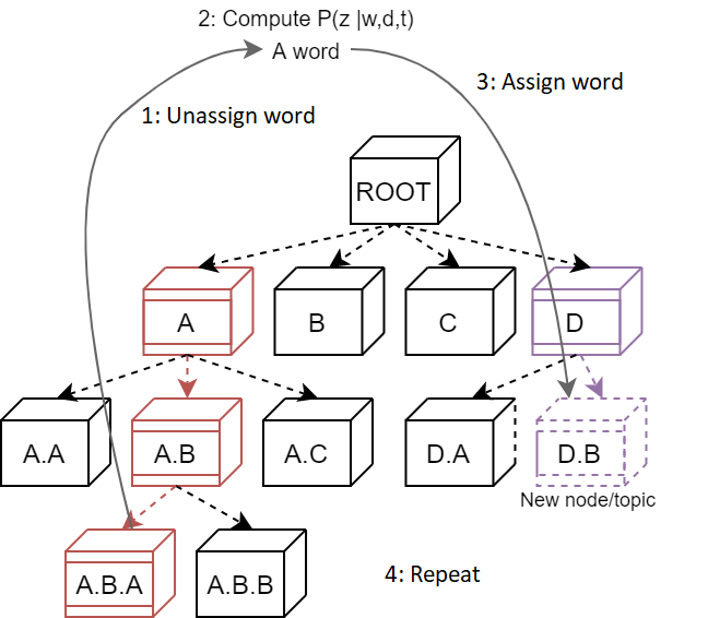
Figure 2: Gibbs sampling with Infinite Dirichlet Trees. Repeat for each word of each document until convergence.

3.3.1 Sampling topic-word assignments (paths in the trees)

We will now explain the procedure behind sampling from the word-topic assignment distribution. When drawing a topic assignment for a word we have three possible outcomes:

1. We draw a node/topic from the associated document tree.

2. We draw a node/topic from the corpus tree.

3. We create a new node/topic.

Formally, given a word $w$ with timestamp $t$ in document $d$, we wish to draw a new topic assignment $z$. As stated in section 3.1, topics are identified as a sequence of node ids. Thus, we iteratively draw the random sequence $z_{0,L}=(z_{0},...,z_{L})$. The length $L$ of this sequence is decided by sampling a Bernoulli distribution in-between the sampling of each $z_{j}$.

Hence each $z_{j}$ is sampled as :

$$z_{j}|w,d,t\sim$$

$$with\ probability\ $$\frac{n_{d}}{\alpha+n_{d}}$$:$$ (3)

$$$$\sum_{k}\frac{\beta_{k}(t)*(A(k|d)+\epsilon)*(A(k|w)+\phi)*\delta_{k}}{(A(k)+(\phi*V))*n_{d}}$$$$ (4)

$$with\ probability\ $$\frac{n_{w}}{\beta+n_{w}}*(\frac{\alpha}{\alpha+n_{d}})$$:$$ (5)

$$$$\sum_{k}\frac{\beta_{k}(t)*(A(k|w)+\phi)*\delta_{k}}{n_{w}}$$$$ (6)

$$with\ probability\ $$\frac{\beta}{\beta+n_{w}}*\frac{\alpha}{\alpha+n_{d}}$$:$$ (7)

$$new\ topic$$ (8)

All the variables are explained in table 4 (Appendix).

Note that sampling a node from the corpus tree can lead to the creation of a new node in the associated document tree if that node does not already exist. However, when creating an entirely new node, it is created in both trees (corpus tree and associated document tree).

Once a topic $z_{j}$ is drawn, we draw from a Bernoulli with parameter $p$ to decide if we stop or go deeper in the tree:

$$p=\frac{P+\theta_{1}}{N+\theta_{1}+\theta_{2}+C+P}$$ (9)

.

$$P=\frac{\beta_{j}(t)*(A^{*}(z_{0,j}|w)+\phi)*(A^{*}(z_{0,j}|d)+\epsilon)}{A^{*}(z_{0,j})+(\phi*V)}$$ (10)

$$N=\frac{\phi*\epsilon}{\phi*V}$$ (11)

$$C=\sum_{k}\frac{\beta_{k}(t)*(A(k|w)+\phi)*(A(k|d)+\epsilon)}{A(k)+(\phi*V)}$$ (12)

All the variables are explained in table 3 (Appendix).

To summarize, when drawing a topic assignment for a word, we either draw from the document tree, corpus tree, or we create a new topic. Then, we draw from a Bernoulli to decide if we go deeper or not. If we do go deeper, we repeat the same process until we eventually stop. This process is then applied repeatedly too all of the words in the corpus multiple times until convergence.

3.4 Comparing HTMOT vs. nHDP

The main difference between HTMOT and nHDP lies in their respective use of the aforementioned Gibbs sampling and SVI training procedures. However, other notable differences exist: First, our HTMOT algorithm starts with all words unassigned whereas nHDP starts with a pre-clustering step using k-means. Second, we do not make use of a greedy algorithm to select trees for each document, i.e, the tree for each document is created automatically as the Gibbs sampler progresses. Hence, our training algorithm is thus simpler and easier to implement by avoiding the need for pre-clustering or greedy procedures.

4 Experimental setup

4.1 Dataset

To perform our experiments, we crawled 62k articles from the Digital Trends archives from 2015 to 2020. This news website is mainly focused on technological news but also contain general news. For all articles, we extracted the text, title and timestamp.

The timestamps are mapped to a number between 0 and 1 which corresponds to the domain of the beta distribution used. Hence, 0 corresponds to the earliest date of a document in the corpus and 1 corresponds to the latest.

We cleaned the data as follows. First, we removed common editor’s sentences such as "we strive to help our readers ….". Then, we relied on Spacy’s NER and POS to filter relevant tokens. Precisely, we kept specific kinds of entities (Person, Norp, Fac, Org, Gpe, Loc, Product, Event, Work_Of_Art, Law, Language) and POS elements (ADJ, NOUN, VERB,INTJ, ADV). Finally, lemmatization was also applied.

A good pre-processing procedure is essential for the interpretability of topics as shown in (Martin and Johnson, 2015). Hence, our extraction of named entities aims at enhancing the topics’ interpretability by showing actors in the topic such as personalities and companies. The training algorithm will not discriminate between words and entities but the visualization interface does. This means that a topic is no longer displayed as a simple list of words but is instead represented by a list of words and a list of entities.

4.2 Parameters

Many parameters control the behavior of our model; this section will describe each of them.

First, we have the Infinite Dirichlet Trees parameters. $\alpha$ : the rate at which we create new topics in the document trees. $\beta$ : the rate at which we create new topics in the corpus tree. $\theta$ : how likely we are to create deeper sub topics.

Second, we have parameters that regulate the growth of the trees. These help speed up the algorithm and keep memory usage to a minimum. CM (Critical Mass) : the minimum valid size of a topic; only valid topics are part of the final output. SM (Splitting Mass) : the minimum size of a topic before it can create sub-topics. Both are defined as a percentage of the total number of words in the corpus. TTL (Time To Live) : how many pass through the corpus before destroying a non-valid node. Nodes are also destroyed when they become empty.

Third, we have the Dirichlet prior parameters as in the traditional LDA model. $\phi$ : the prior for the topic-word distribution. $\epsilon$ : the prior for the corpus and document-topic distributions.

Finally, we have training parameters. Iterations : how many batches we will go through during training. SGI (Stop Growth Iteration) : a point at which node new nodes won’t be created. Set SGI $<$ Iterations to ensure that the last topic to be created has time to converge.

Table 1 defines the value of each parameter used to perform our experiments.

5 Results and Discussion

We now present our results, starting with a statistical analysis of the training behavior of HTMOT. Then, we will discuss the results of the Word Intrusion task, its drawbacks and directions for future topic modelling evaluation methods. Finally, we will examine the various extracted topics qualitatively.

5.1 Convergence rate, training speed and algorithmic complexity

We assessed the convergence of our method by looking at the frequency of topics over time during training. This frequency indicates how many words in the corpus are assigned to each topic. As these frequencies stabilise (the curves flatten), this indicates that the model converged. However, as hierarchical topic models extract hundreds of topics, observing the frequency of each topic is not reasonable. Thus, we only observe the convergence of depth 1 topics.

We observed that the convergence rate of our training algorithm is sub-linear with respect to the dataset size. These experiments were performed by using samples of the full dataset. Specifically, using a dataset which is ten time smaller leads to a halving of the time to convergence. However new topics created during training will perturb this convergence. Hence, we prevent this issue with the SGI parameter (see section 4.2) which provides a period at the end of training where no topics can be created.

Now let’s consider actual training time of our training procedure with respect to the nHDP’s SVI procedure. Unlike our method (HTMOT), nHDP lacks a temporal component. Therefore, to ensure a fair comparison in our experiments, we disabled HTMOT’s temporal modelling. We observed that our sampler analyses 135k documents per hour . For nHDP, based on the figures reported in Paisley et al. (2015), we can estimate that SVI analyses roughly 90k articles per hour (Paisley et al., 2015) . Hence, we believe that our training algorithm is comparable to nHDP’s SVI in term of speed. This observations contradicts previous wisdom that SVI is considerably faster than gibbs sampling Paisley et al. (2015). Overall our model achieved convergence after 10h of training on the full dataset.

We observed that the algorithmic complexity is linear with respect to the dataset size. However, the depth of the topic trees and, thus, the growth and regulating parameters for the IDTs can greatly impact performance.

5.2 Results of the Word Intrusion task

We applied the Word Intrusion task to evaluate our model. The original Word Intrusion task involves selecting an intruder word from any other topic. However, since our model is hierarchical, we decided to select intruder words from sibling topics only. This makes the task more difficult as deeper topics tend to be more lexically related to their siblings. This is important as we want topics to be distinct from their siblings. Let’s take the example of selecting an intruder word for the sub-topic of "astronomy". In the classical Word Intrusion task, we could choose any topic such as the "Covid-19 vaccines" topic (see figure 3). In our case, we would choose from one of its siblings such as the "astronaut" topic instead. Hence, the chosen intruder is semantically much closer to the target topic "astronomy". Thus, this provides a more robust evaluation of topic quality.

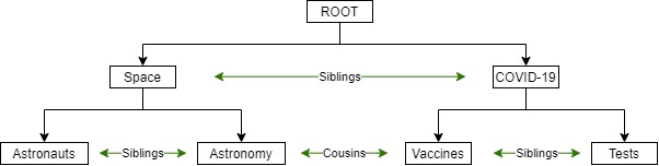
Figure 3: Example of a topic tree with cousins and siblings.

We performed this task using a survey created with Google Forms . The survey required annotators to select an intruder word for each topic presented and provide a confidence score for each answer. The annotators come from an internet community involved in sharing and answering surveys . 57 respondents answered the survey over the month of may 2021.

Results show 74.83% accuracy in the Word Intrusion task (as defined in section 2.4) on 6 topics at various depths. We have also used the automated the word intrusion by replicating the method of Lau et al. (2014). We observed an accuracy of 79%. Hence, both automated and non-automated methods show results on par with LDA’s performance shown in the original Word Intrusion task paper (Chang et al., 2009).

5.3 Qualitative examination of the resulting topics

Now, we will inspect a selection of topics to illustrate the capabilities of our HTMOT model. Specifically, we will focus on the high level topic of space exploration and its sub-topics.

Figure 7 presents a depth 1 topic and two of its sub-topics. We can clearly see that the parent topic is about space, and the two sub-topics are about astronomy and astronauts , which are indeed related to the parent topic. This example also illustrates how entities can help interpret and understand these topics. For example, in the astronauts topic, we can see that Bob Behnken, (Doug) Hurley and SpaceX are important entities. A quick look at the top documents for that topic show that they were the first to fly on a SpaceX rocket. Moreover, in the astronomy topic, Hubble and Spitzer are frequent entities. This is coherent as they are two important low earth orbit telescopes. Other sub-topics of space include satellite launches, rovers, exoplanets, test flights, etc.

Figure 4 shows an example of temporality and hierarchy working together. In this representation, we can see the estimated time distributions (we show the years 2020 and 2021 to have smaller charts). Here, we have the sub-topic of astronauts and its own three sub-topics: the historic test launch of the spaceX Dragon capsule, the crew 1 launch and the crew 3 launch. These topics were interpreted mostly from top documents. This is because at these depth topics become so small they are difficult to interpret based on top words as they are so precise. These topics are depth 3 topics which means temporal modelling is enabled. We can see that they are well localized in time as their associated time distribution is narrow. The estimated time distribution of the sub-topics matches the timing of the aforementioned events : May 2020, November 2020 and November 2021. This demonstrates that the ability of our model to extract atomic events at the deeper level of the tree. Noticeably, the model did not extract the crew 2 launch event. However, this might be explained by the fact that the digital trends news outlet saw a sharp decline in articles output during this period as can be seen in figure 6.

Now, we will look at the document tree for one document, see figure 5. This was created by choosing only the topics that were assigned to at least 5% of words in the chosen document. The document in question is titled "Astronauts are using VR to train for the Boeing Starliner capsule". The three main extracted topics are virtual reality applications, space and R&D. Two children of the topic of space were also assigned to this document: test and astronauts. From the title, it can be seen that the tree captures the main themes of this document.

6 Conclusion

We have proposed a new model for topic modelling capable of modelling hierarchy and time jointly. Through examples, we have demonstrated how combining hierarchy and temporality provides us with a more fine grained understanding of a corpus through detailed sub-topics which can represent specific events. Moreover, we developed a novel implementation of Gibbs sampling for hierarchical topic models. This implementation provides a fast alternative to SVI that makes Gibbs sampling a viable solution for training such complex models. Moreover, we have shown how extracting entities can help interpret and understand topics at a deeper level.

7 Limitations

Our model is subject to a few limitations that lays the foundations for future work. We have inherited the general limitations existing in all topic models techniques.

• As topic models require tokenization, non-tokenizable languages like Chinese are not compatible

• Since we cannot be aware of all the content of the training corpus, it is difficult to determine if some topics were missed during extraction; we can only evaluate the topics that are extracted.

• Hyper parameters defining priors on probability distributions may depend on the specifics of the dataset such as the number of articles, their average length or how varied/narrow a corpus is (affecting the number of topics to expect)

• Topics must be interpreted by humans which is not always a simple task even with additional information such as top entities or top documents

We also have limitations that are specific to our method

• Convergence must be observed to confirm the end of the training phase. However, as hierarchical topic model can extract hundreds of topics, we cannot ensure the convergence of each topic manually and only asses the first level topics.

• The deeper a topic is, the more esoteric it becomes. Hence, it can be difficult to interpret such topics as it require specific domain knowledge.

• Since we cannot be aware of all the content of the training corpus, it is difficult to determine if some events (topics localized in time) were missed during extraction. we can only evaluate the events that are extracted.

Appendix A Tables and figures

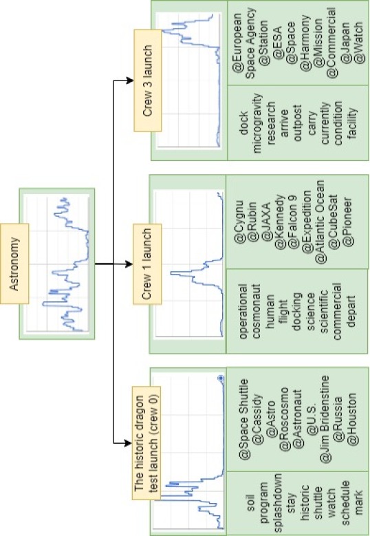
Figure 4: Examples of depth 3 topics that are well localized in time

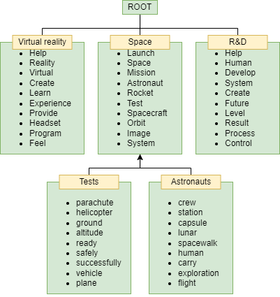
Figure 5: Example of document topic tree for the document : "Astronauts are using VR to train for the Boeing Starliner capsule" .

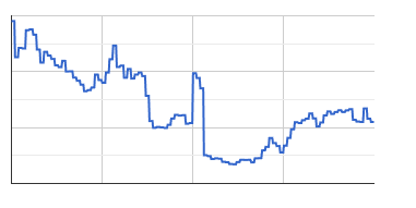
Figure 6: Number of articles published by Digital Trends over the years 2020 and 2021. We can see a sharp decline at the beginning of the year 2021 (middle of the graph)

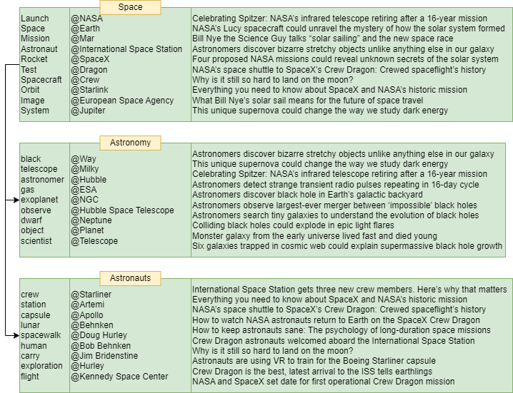
Figure 7: The space topic and two of its sub-topics : astronauts and astronomy. Each topics is shown with top words (left), top entities (center) and top documents (right)

Name	Value	Category
$\alpha$	0.00005	IDTs parameters
$\beta$	0.0002
$\theta$	0.25
Critical Mass (CM)	0.0005	IDTs growth control
Splitting Mass (SM)	0.005
Time To Live (TTL)	2
$\phi$	0.1	Traditional LDA topic parameters
$\epsilon$	1
Iterations	4500	Training parameters
Batch size	500

Table 1: Parameters used for our model

Model name	Type	Reference	Corpora
LDA	Classic	(Blei et al., 2003)	News articles
HDP	Classic	(Teh et al., 2006)	Scientific papers
nCRP	Hierarchical	(Blei et al., 2004)	Abstracts
PAMmix	Hierarchical	(Mimno et al., 2007)	Abstracts
nHDP	Hierarchical	(Paisley et al., 2015)	News articles and Wikipedia
LSHTM	Hierarchical	(Pujara and Skomoroch, 2012)	News articles and Wikipedia
DTM	Temporal	(Blei and Lafferty, 2006)	Scientific papers
ToT	Temporal	(Wang and McCallum, 2006)	Scientific papers, mails and historical texts
MTT	Temporal	(Nallapati et al., 2007)	News articles
DCTM	Temporal	(Song et al., 2008)	Scientific papers

Table 2: Related methods corpora, evaluation methods used and type of topic model.

Variable	Description
$A^{*}(z_{0,j})$	# words assigned to topic $z_{0,j}$
P	Weight of the currently selected node $z_{0,j}$.
C	Weight of all of the children of the selected node $z_{0,j}$.
N	Weight of a potentially new child for $z_{0,j}$
$\theta_{1}$ and $\theta_{2}$	Prior for the Bernoulli distribution

Table 3: Descriptions of variables for equations 9 to 12

Variable	Description
$n$	# words in the corpus
$n_{d}$	# words in the corpus that are part of document $d$
$n_{w}$	# words in the corpus that are instantiations of the word $w$
V	Vocabulary length
$A(k|w)$	# words $w$ assigned to topic $(z_{0,j-1},k)$ or its descendants (corpus tree information)
$A(k|d)$	# words in document $d$ assigned to topic $(z_{0,j-1},k)$ or its descendants (document tree information)
$A(k)$	# words assigned to topic $(z_{0,j-1},k)$ or its descendants
$\beta_{k}$	Probability density function of the beta distribution with parameter $\rho^{1}_{k}$ and $\rho^{2}_{k}$ associated with topic $(z_{0,j-1},k)$
$\epsilon,\phi,\beta,\alpha$	Priors for the Dirichlet distributions and processes (more details are provided in the parameter section)

Table 4: Descriptions of variables for equations 3 to 8

References

- Alghamdi and Alfalqi (2015) Rubayyi Alghamdi and Khalid Alfalqi. 2015. A survey of topic modeling in text mining. International Journal of Advanced Computer Science and Applications, 6(1).
- Barde and Bainwad (2017) Bhagyashree Vyankatrao Barde and Anant Madhavrao Bainwad. 2017. An overview of topic modeling methods and tools. In 2017 International Conference on Intelligent Computing and Control Systems (ICICCS). IEEE.
- Bastani et al. (2019) Kaveh Bastani, Hamed Namavari, and Jeffrey Shaffer. 2019. Latent dirichlet allocation (lda) for topic modeling of the cfpb consumer complaints. Expert Systems with Applications, 127:256–271.
- Blei et al. (2004) David M Blei, Thomas L Griffiths, Michael I Jordan, and Joshua B Tenenbaum. 2004. Hierarchical topic models and the nested chinese restaurant process. Advances in neural information processing systems, 16(16):17–24.
- Blei et al. (2017) David M. Blei, Alp Kucukelbir, and Jon D. McAuliffe. 2017. Variational inference: A review for statisticians. Journal of the American Statistical Association, 112(518):859–877.
- Blei and Lafferty (2006) David M Blei and John D Lafferty. 2006. Dynamic topic models. In Proceedings of the 23rd international conference on Machine learning, pages 113–120.
- Blei et al. (2003) David M. Blei, Andrew Y. Ng, and Michael I. Jordan. 2003. Latent dirichlet allocation. J. Mach. Learn. Res., 3(null):993–1022.
- Chang et al. (2009) Jonathan Chang, Sean Gerrish, Chong Wang, Jordan Boyd-graber, and David Blei. 2009. Reading tea leaves: How humans interpret topic models. In Advances in Neural Information Processing Systems, volume 22, pages 288–296. Curran Associates, Inc.
- El Akrouchi et al. (2021) Manal El Akrouchi, Houda Benbrahim, and Ismail Kassou. 2021. End-to-end lda-based automatic weak signal detection in web news. Knowledge-Based Systems, 212:106650.
- Gregoriades et al. (2021) Andreas Gregoriades, Maria Pampaka, Herodotos Herodotou, and Evripides Christodoulou. 2021. Supporting digital content marketing and messaging through topic modelling and decision trees. Expert Systems with Applications, 184:115546.
- Hong et al. (2011) Liangjie Hong, Dawei Yin, Jian Guo, and Brian D. Davison. 2011. Tracking trends: Incorporating term volume into temporal topic models. In Proceedings of the 17th ACM SIGKDD International Conference on Knowledge Discovery and Data Mining, KDD ’11, page 484–492, New York, NY, USA. Association for Computing Machinery.
- Hoyle et al. (2021) Alexander Miserlis Hoyle, Pranav Goel, Denis Peskov, Andrew Hian-Cheong, Jordan L. Boyd-Graber, and Philip Resnik. 2021. Is automated topic model evaluation broken?: The incoherence of coherence. CoRR, abs/2107.02173.
- Kim et al. (2020) Suhyeon Kim, Haecheong Park, and Junghye Lee. 2020. Word2vec-based latent semantic analysis (w2v-lsa) for topic modeling: A study on blockchain technology trend analysis. Expert Systems with Applications, 152:113401.
- Korfiatis et al. (2019) Nikolaos Korfiatis, Panagiotis Stamolampros, Panos Kourouthanassis, and Vasileios Sagiadinos. 2019. Measuring service quality from unstructured data: A topic modeling application on airline passengers’ online reviews. Expert Systems with Applications, 116:472–486.
- Lau et al. (2014) Jey Han Lau, David Newman, and Timothy Baldwin. 2014. Machine reading tea leaves: Automatically evaluating topic coherence and topic model quality. In Proceedings of the 14th Conference of the European Chapter of the Association for Computational Linguistics, pages 530–539, Gothenburg, Sweden. Association for Computational Linguistics.
- Martin and Johnson (2015) Fiona Martin and Mark Johnson. 2015. More efficient topic modelling through a noun only approach. In Proceedings of the Australasian Language Technology Association Workshop 2015, pages 111–115, Parramatta, Australia.
- Mimno et al. (2007) David Mimno, Wei Li, and Andrew McCallum. 2007. Mixtures of hierarchical topics with pachinko allocation. In Proceedings of the 24th international conference on Machine learning, pages 633–640.
- Nallapati et al. (2007) Ramesh M Nallapati, Susan Ditmore, John D Lafferty, and Kin Ung. 2007. Multiscale topic tomography. In Proceedings of the 13th ACM SIGKDD international conference on Knowledge discovery and data mining, pages 520–529.
- Paisley et al. (2015) J. Paisley, C. Wang, D. M. Blei, and M. I. Jordan. 2015. Nested hierarchical dirichlet processes. IEEE Transactions on Pattern Analysis and Machine Intelligence, 37(2):256–270.
- Pujara and Skomoroch (2012) Jay Pujara and Peter Skomoroch. 2012. Large-scale hierarchical topic models. In NIPS Workshop on Big Learning, volume 128.
- Song et al. (2008) Yang Song, Lu Zhang, and C Lee Giles. 2008. A non-parametric approach to pair-wise dynamic topic correlation detection. In 2008 Eighth IEEE International Conference on Data Mining, pages 1031–1036. IEEE.
- Teh et al. (2006) Yee Whye Teh, Michael I Jordan, Matthew J Beal, and David M Blei. 2006. Hierarchical dirichlet processes. Journal of the American Statistical Association, 101(476):1566–1581.
- Wang et al. (2019) Hei-Chia Wang, Tzu-Ting Hsu, and Yunita Sari. 2019. Personal research idea recommendation using research trends and a hierarchical topic model. Scientometrics, 121(3):1385–1406.
- Wang and McCallum (2006) Xuerui Wang and Andrew McCallum. 2006. Topics over time: A non-markov continuous-time model of topical trends. In Proceedings of the 12th ACM SIGKDD International Conference on Knowledge Discovery and Data Mining, KDD ’06, page 424–433, New York, NY, USA. Association for Computing Machinery.
- Xiao and Stibor (2010) Han Xiao and Thomas Stibor. 2010. Efficient collapsed gibbs sampling for latent dirichlet allocation. In Proceedings of 2nd Asian Conference on Machine Learning, volume 13 of Proceedings of Machine Learning Research, pages 63–78, Tokyo, Japan. JMLR Workshop and Conference Proceedings.
- Yang et al. (2015) Guangbing Yang, Dunwei Wen, Kinshuk, Nian-Shing Chen, and Erkki Sutinen. 2015. A novel contextual topic model for multi-document summarization. Expert Systems with Applications, 42(3):1340–1352.
- Zhou and Chen (2013) Xiangmin Zhou and Lei Chen. 2013. Event detection over twitter social media streams. The VLDB Journal, 23(3):381–400.
- Zhu et al. (2017) Xiaofeng Zhu, Diego Klabjan, and Patrick N. Bless. 2017. Unsupervised terminological ontology learning based on hierarchical topic modeling. In 2017 IEEE International Conference on Information Reuse and Integration (IRI), pages 32–41.