Deep Quantile and Deep Composite Model Regression

Abstract

A main difficulty in actuarial claim size modeling is that there is no simple off-the-shelf distribution that simultaneously provides a good distributional model for the main body and the tail of the data. In particular, covariates may have different effects for small and for large claim sizes. To cope with this problem, we introduce a deep composite regression model whose splicing point is given in terms of a quantile of the conditional claim size distribution rather than a constant. To facilitate M-estimation for such models, we introduce and characterize the class of strictly consistent scoring functions for the triplet consisting a quantile, as well as the lower and upper expected shortfall beyond that quantile. In a second step, this elicitability result is applied to fit deep neural network regression models. We demonstrate the applicability of our approach and its superiority over classical approaches on a real accident insurance data set.

JEL Codes. C14; C31; C450; C510; C520; C580

Keywords. Elicitability, consistent loss function, proper scoring rule, Bregman divergence, pinball loss, quantile regression, expected shortfall regression, conditional tail expectation, neural network regression, deep composite regression, splicing model, mixture model.

1 Introduction

1.1 Background

In actuarial modeling, we typically use regression models to estimate expected values of claim sizes exploiting systematic effects of features or covariates. These estimated expected values are used for insurance pricing, claims forecasting and claims reserving. The most commonly used regression model is the generalized linear model (GLM) with the exponential dispersion family (EDF) as the underlying distributional model. Parameter estimation within this EDF-GLM framework is performed by maximum likelihood estimation (MLE). In this setup, MLE is equivalent to minimizing the corresponding deviance loss function, the latter being a strictly consistent scoring function for mean. Strictly consistent scoring functions facilitate M-estimation and forecast evaluation; further details are provided below. For actuarial problems, there are three main issues with this approach:

• The EDF only contains light-tailed distribution functions such as the Gaussian, the Poisson, the gamma or the inverse Gaussian distributions. For this reason, the classical EDF-GLM framework is not suitable if we have a mixture of light-tailed and heavy-tailed data. This fact is often disregarded in practice and the EDF-GLM framework is used nevertheless. This may result in over-fitting to large claims and non-robustness in model estimation.

• The GLM regression structure may not be suitable or covariate engineering may be too difficult to bring the regression problem into a GLM form. As a result, not all systematic effects such as interactions may be correctly incorporated into the GLM.

• The GLM is usually used to estimate expected values. From a risk management perspective, one is also interested in other quantities such as quantiles and expected shortfalls (ES). If the aforementioned distributional model within the EDF is not suitable for the description of the observed data, then a very accurately estimated expected value is not directly helpful in estimating quantiles and ES.

Our paper tackles the above points; we first discuss the related literature and then we are going to describe our proposal. To deal with the problem of the lack of any simple off-the-shelf distribution that fits the entire range of the data, i.e., the body and tail of the data, one often either uses a composite (splicing) model or a mixture model. These two approaches can be fitted with the expectation-maximization (EM) algorithm. Composite models are studied in Cooray–Ananda [2], Scollnik [32], Pigeon–Denuit [28], Grün–Miljkovic [15] and Parodi [27]. These papers do not consider a regression structure and covariates. The only actuarial publications that we are aware of considering composite regression models are Gan–Valdez [11] and Laudagé et al. [21]. Both proposals choose very specific distributional assumptions above and below a given threshold (splicing point) to obtain analytical tractability. In our proposal, we do not fix the threshold itself, but a quantile level instead. This allows us for direct model fitting below and above that quantile, and, moreover, we can have a flexible regression structure for both the body and the tail of the data. For mixture models, not considered in this paper, we refer to Fung et al. [10] and the literature therein. Both approaches, composite and mixture models, typically use the EM algorithm for model fitting. Our approach is based on the (simpler) stochastic gradient descent (SGD) algorithm.

Focusing on point (2) from above, there are several ways in extending (or modifying) a GLM. These include, e.g., generalized additive models (GAMs), regression trees and tree boosting, or feed-forward neural (FN) network regression models; we refer to Hastie et al. [18]. Here, we focus on FN network regression models as a straightforward and powerful extension of GLMs. Moreover, we see that an FN network architecture can easily be designed so that it can simultaneously fulfill different estimation tasks. This is a crucial property that we need in our derivations, as we jointly estimate different regression models for the body and tail of the data.

Concerning point (3) from above, quantile regression has gained quite some popularity in the machine learning community to quantify uncertainty, see Meinshausen [23] and Takeuchi et al. [33]. Quantile regression has been introduced by Koenker–Bassett [20], and it is widely used in statistical modeling these days; for a recent monograph we refer to Uribe–Guillen [36]. Our proposal extends the approach of Richman [29] who combines joint estimation of a quantile and the mean within an FN network architecture, see Listing 8 in Richman [29].

1.2 Proposed method

We consider two different, though closely related problems in this paper. On the one hand, we extend the work of Richman [29] by proposing an FN network architecture that allows for consistent multiple quantile regression respecting monotonicity of the quantiles at different levels. On the other hand, this FN network architecture is at the basis of the extension of the joint quantile and ES regression considered in Guillen et al. [16]. The main building blocks in our estimation procedure are strictly consistent scoring functions for our target functionals. These are functions of the estimated model prediction and the response variable which are minimised in expectation by the correctly specified model. Strictly consistent scoring functions are at the core of consistent M-estimation (where M stands for minimisation) in a regression setup, see Dimitriadis et al. [4]. If a target functional admits a strictly consistent scoring function, it is called elicitable. The elicitability of the mean and the quantile thus allow for mean and quantile regression, using the squared loss (or a Bregman divergence) or the pinball loss (or a generalized piecewise linear loss), respectively. In model selection and, more generally, forecast ranking, Gneiting [12] and Gneiting–Raftery [14] advocate for the usage of strictly consistent scoring functions since they honour honest and truthful forecasts.

In a first step, we perform multiple quantile regression using the sum of pinball losses as strictly consistent scoring functions. Since quantiles are monotone in their probability levels, we modify the FN network architecture of Richman [29] such that we can guarantee this monotonicity.

In a second step, we extend the work of Guillen et al. [16] in several ways. In risk management, besides knowing quantiles, one is also interested in estimating ES, which reflects the average outcome beyond the quantile. Since ES is not elicitable [12], stand-alone ES regression is generally not possible. Fissler–Ziegel [6] showed that the pair of ES together with the quantile at the same probability level is elicitable. This paved the way to joint quantile–ES regression, see Dimitriadis–Bayer [3] and Guillen et al. [16] for (G)LM approaches. We first extend the result of Fissler–Ziegel [6], showing the elicitability of the composite triplet consisting of a quantile together with the lower and upper ES at the same probability level, and characterizing the entire class of strictly consistent scoring functions for it. Hence, we are in the position to estimate a full composite regression model in a one-step procedure. This is in contrast to the two-step estimation approach of Barendse [1], first estimating the quantile and then in a second step the ES below and above the quantile. Such a two-step estimation approach becomes problematic in the presence of common parameters in the three components of the regression model. Second, we motivate the particular choice of the strictly consistent scoring function in a data-driven manner, striving for efficient parameter estimation. To this end, we use optimality results known for mean regression which are akin to the optimality results derived in Dimitriadis et al. [4] for the pair of the quantile and ES. The third novelty we provide is the FN network architecture that respects the necessary monotonicity property of the composite triplet in an estimation context. This architecture can directly be fitted using the stochastic gradient descent (SGD) algorithm. This fitting approach does neither require a two-step fitting approach nor the EM algorithm as it is used in related problems. Moreover, our fitting turns out to be robust, and we do not encounter the stability issues as in the two-step approaches and the EM algorithm.

Organization of this manuscript. In Section 2 we review the concepts of strictly consistent scoring functions used in estimation and forecast evaluation. We recall known characterization results of strictly consistent scores for the mean and for the quantile. We extend the results of Fissler–Ziegel [6] introducing the class of strictly consistent scoring functions for the composite triplet of the quantile, lower ES and upper ES at the same probability level. In Section 3 we discuss how these quantities can be estimated within a neural network regression framework, and we also discuss asymptotically efficient choices of scoring functions. In Section 4 we give a real data example which demonstrates the suitability of our proposal. Section 5 concludes and provides an outlook to related open problems.

2 Statistical learning

2.1 A review of strictly consistent scoring functions

We start from the decision-theoretic approach of forecast evaluation developed by Gneiting [12] and Gneiting–Raftery [14], also used for M-estimation in Dimitriadis et al. [4]. This provides us with suitable choices of scoring functions for model fitting, model selection, and forecast evaluation. Denote by ${\cal F}$ the class of considered distribution functions $F\in{\cal F}$. Let ${\mathbb{Y}}\subseteq{\mathbb{R}}$ be an interval, a halfline or the whole real line ${\mathbb{R}}$, such that the support of each $F\in{\cal F}$ is contained in ${\mathbb{Y}}$. Choose an action space ${\mathbb{A}}\subseteq{\mathbb{R}}$ from which we select actions $a\in{\mathbb{A}}$ to estimate a statistics $A(F)\in{\mathbb{A}}$ of $F\in{\cal F}$. That is, we have a functional

$$A:{\cal F}\to{\mathbb{A}}\qquad F\mapsto A(F),$$ (2.1)

that we try to estimate. Commonly used functionals are the mean functional $A(F)={\mathbb{E}}_{F}[Y]$ for $Y\sim F\in{\cal F}$ and quantiles. Given a probability level $\tau\in(0,1)$, the $\tau$-quantile of $F\in{\cal F}$ is given by the (left-continuous) generalized inverse

$$A(F)=F^{-1}(\tau)=\inf\left\{y\in{\mathbb{R}};~{}F(y)\geq\tau\right\}.$$ (2.2)

To receive an intuitive understanding we usually speak about a functional (2.1) that attains a single value $A(F)$ in the action space ${\mathbb{A}}$. Often this functional is obtained by an optimization (M-estimator), or by finding the roots of a given function (Z-estimator). Since, in general, we do not want to assume uniqueness of such a solution, we should understand this functional as a set-valued map

$$A:{\cal F}\to{\cal P}({{\mathbb{A}}})\qquad F\mapsto A(F)\subset{\mathbb{A}},$$ (2.3)

where ${\cal P}({{\mathbb{A}}})$ is the power set of ${\mathbb{A}}$. E.g., the set-valued $\tau$-quantile of a distribution $F$ is given by

$$q_{\tau}(F)=\{t\in{\mathbb{R}}\colon F(t-)\leq\tau\leq F(t)\},$$ (2.4)

where $F(t-)=\lim_{x\uparrow t}F(x)$. This defines a closed interval and its lower endpoint corresponds to the left-continuous generalized inverse $F^{-1}(\tau)$ given in (2.2). To keep notation simple, we identify $\widehat{a}$ and $A(F)$ if $A(F)=\{\widehat{a}\}$ is a singleton.

In order to evaluate the accuracy of actions $a$ for the statistics $A(F)$ (for unknown $F$) we consider a scoring function (also called loss function)

$$L:{\mathbb{Y}}\times{\mathbb{A}}\to{\mathbb{R}},\qquad(y;a)\mapsto L(y;a).$$

This describes the loss of an action $a\in{\mathbb{A}}$ if a realization $y$ of $Y\sim F$ materializes. To incentivize truthful forecasts, Gneiting [12] advocates that this scoring function $L$ should be strictly consistent for the functional $F\mapsto A(F)$ of interest.

Definition 2.1 (strict consistency)

A scoring function $L:{\mathbb{Y}}\times{\mathbb{A}}\to{\mathbb{R}}$ is ${\cal F}$-consistent for a given functional $A:{\cal F}\to{\cal P}({\mathbb{A}})$ if ${\mathbb{E}}_{F}\left[|L(Y;a)|\right]<\infty$ for all $Y\sim F\in{\cal F}$ and for all $a\in{\mathbb{A}}$ and if

$${\mathbb{E}}_{F}\left[L(Y;\widehat{a})\right]~{}\leq~{}{\mathbb{E}}_{F}\left[L(Y;a)\right],$$ (2.5)

for all $Y\sim F\in{\cal F}$, $\widehat{a}\in A(F)$ and $a\in{\mathbb{A}}$. It is strictly ${\cal F}$-consistent if it is ${\cal F}$-consistent and equality in (2.5) implies that $a\in A(F)$.

Gneiting [12] shows that strictly consistent scoring functions are linked to proper scoring rules, which serve to evaluate probabilistic forecasts (i.e. actions $a$ taking the form of probability distributions) and which are discussed in detail in Gneiting–Raftery [14]. On the estimation side, we also need (strict) consistency of scoring functions to obtain consistency of M-estimators, see Chapter 5 in Van der Vaart [37] and Dimitriadis et al. [4]. This raises the question of which functionals $A:{\cal F}\to{\mathbb{A}}$ admit strictly consistent scoring functions $L$, i.e., are elicitable.

Definition 2.2 (elicitable)

The functional $A:{\cal F}\to{\cal P}({\mathbb{A}})$ is elicitable on a given class of distribution functions ${\cal F}$ if there exists a scoring function $L$ that is strictly ${\cal F}$-consistent for $A$.

The general question of elicitability is studied and discussed in detail in Gneiting [12]. For instance, the mean functional $A(F)={\mathbb{E}}_{F}[Y]$ and the $\tau$-quantile $q_{\tau}$ defined in (2.4) are elicitable; see Theorems 2.3 and 2.4, below. We start with useful properties of scoring functions $L$ that are going to be used in the next theorems. Assume ${\mathbb{Y}}={\mathbb{A}}\subseteq{\mathbb{R}}$ is an interval with non-empty interior. We set:

• $L(y;a)\geq 0$ and equality holds if and only if $y=a$;

• $L(y;a)$ is measurable in $y$ and continuous in $a$;

• The partial derivative $\partial_{a}L(y;a)$ exists and is continuous in $a$ whenever $a\neq y$.

These regularity conditions can often be weakened. Especially the positivity in (S0) can be relaxed. However, it is a nice property to have in optimizations as it gives us a natural lower bound to the minimal score that can be achieved.

The following result goes back to Savage [31].

Theorem 2.3 (Gneiting [12], Theorem 7)

Let ${\cal F}$ be a class of distribution functions on interval ${\mathbb{Y}}\subseteq{\mathbb{R}}$ with finite first moment.

• The mean functional $F\mapsto A(F)={\mathbb{E}}_{F}[Y]$ is elicitable relative to ${\cal F}$.

• Assume the scoring function $L:{\mathbb{Y}}\times{\mathbb{A}}\to{\mathbb{R}}_{+}$ satisfies (S0)–(S2) for an interval ${\mathbb{Y}}={\mathbb{A}}\subseteq{\mathbb{R}}$ and that ${\cal F}$ is the class of compactly supported distributions on ${\mathbb{Y}}$. The scoring function $L$ is ${\cal F}$-consistent for the mean functional if and only if $L$ is of the form

  $$L(y;a)=L_{\phi}(y;a)=\phi(y)-\phi(a)-\phi^{\prime}(a)\left(y-a\right),$$ (2.6)

  for a convex function $\phi$ with (sub-)gradient $\phi^{\prime}$ on ${\mathbb{Y}}$.

• If $\phi$ is strictly convex on ${\mathbb{Y}}$, then scoring function (2.6) is strictly consistent for the mean functional on the class ${\cal F}$ of distribution functions $F$ on ${\mathbb{Y}}$ for which both ${\mathbb{E}}_{F}[Y]$ and ${\mathbb{E}}_{F}[\phi(Y)]$ exist and are finite.

The maps $L_{\phi}$ defined in (2.6) are called Bregman divergences and, basically, the previous theorem says that all strictly consistent scoring functions for the mean functional are Bregman divergences. The most prominent Bregman divergence arises by setting $\phi(y)=y^{2}$, yielding the squared loss $L(y;a)=(y-a)^{2}$. On the other hand, the variance functional $\mathbb{V}_{F}(Y)$ is not elicitable (Gneiting [12] and Osband [26]), i.e., there does not exist any strictly consistent scoring function for estimating the variance according to a minimization (2.5).

The following elicitability results for quantiles (2.4) originates from Thomson [34] and Saerens [30].

Theorem 2.4 (Gneiting [12], Theorem 9)

Let ${\cal F}$ be a class of distribution functions on interval ${\mathbb{Y}}\subseteq{\mathbb{R}}$ and choose $\tau\in(0,1)$.

• The $\tau$-quantile (2.4) is elicitable relative to ${\cal F}$.

• Assume the scoring function $L:{\mathbb{Y}}\times{\mathbb{A}}\to{\mathbb{R}}_{+}$ satisfies (S0)–(S2) for an interval ${\mathbb{Y}}={\mathbb{A}}\subseteq{\mathbb{R}}$ and that ${\cal F}$ is the class of compactly supported distributions on ${\mathbb{Y}}$. The scoring function $L$ is ${\cal F}$-consistent for the $\tau$-quantile (2.4) if and only if $L$ is of the form

  $$L_{\tau}(y;a)=\left(g(y)-g(a)\right)\left(\tau-\mathds{1}_{\{y\leq a\}}\right),$$ (2.7)

  for a non-decreasing function $g$ on ${\mathbb{Y}}$.

• If $g$ is strictly increasing on ${\mathbb{Y}}$ and ${\mathbb{E}}_{F}[g(Y)]$ exists and is finite for all $F\in\mathcal{F}$, then $L$ defined by (2.7) is strictly ${\cal F}$-consistent for the $\tau$-quantile (2.4).

Members of the class (2.7) are called generalized piecewise linear losses, see Gneiting [13]. Basically, it is this theorem that allows us to consider quantile regression, introduced by Koenker–Bassett [20], as it tells us that quantiles can be estimated from strictly consistent scoring functions. This is going to be outlined below. There is still the freedom of the choice of the strictly increasing function $g$. The most commonly used choice is the identity function $g(y)=y$. This then provides us with the so-called pinball loss for given probability level $\tau\in(0,1)$

$$L_{\tau}(y;a)=(y-a)\left(\tau-\mathds{1}_{\{y\leq a\}}\right)~{}\geq~{}0.$$ (2.8)

In view of Theorem 2.4, the choice of pinball loss requires that ${\cal F}$ contains only distributions with a finite first moment.

We introduce scoring functions closely related to the pinball loss (2.8) where the positivity assumption (S0) has been relaxed:

$$S^{-}_{\tau}(y;a) =\left(\mathds{1}_{\{y\leq a\}}-\tau\right)a-\mathds{1}_{\{y\leq a\}}y,$$

$$S^{+}_{\tau}(y;a) =\left(1-\tau-\mathds{1}_{\{y>a\}}\right)a+\mathds{1}_{\{y>a\}}y,$$

for $y,a\in{\mathbb{R}}$ and for $\tau\in(0,1)$. Note that $S^{+}_{\tau}(y;a)=S^{-}_{\tau}(y;a)+y$, moreover, it holds for the pinball loss

$$L_{\tau}(y;a)=S^{-}_{\tau}(y;a)+\tau y=S^{+}_{\tau}(y;a)-(1-\tau)y.$$

An immediate consequence from Theorem 2.4 is the following corollary.

Corollary 2.5

Let $\mathcal{F}$ contain only distributions with finite first moments. Then $S^{-}_{\tau}$ and $S^{+}_{\tau}$ are strictly $\mathcal{F}$-consistent for the $\tau$-quantile (2.4), that is,

$$q_{\tau}(F)=\operatorname*{arg\,min}_{a\in{\mathbb{R}}}\mathbb{E}_{F}\big{[}S^{-}_{\tau}(Y;a)]=\operatorname*{arg\,min}_{a\in{\mathbb{R}}}\mathbb{E}_{F}\big{[}S^{+}_{\tau}(Y;a)]=\operatorname*{arg\,min}_{a\in{\mathbb{R}}}\mathbb{E}_{F}\big{[}L_{\tau}(Y;a)].$$ (2.9)

Observe that the three functions $S^{-}_{\tau}$ $S^{+}_{\tau}$ and $L_{\tau}$ only differ in terms that do not depend on $a$, and therefore the argument of these minimizations is the same. The pinball loss $L_{\tau}(y;a)$ has the advantage to satisfy condition (S0).

2.2 Expected shortfall and the composite triplet

From the previous section we know that we can estimate $\tau$-quantiles (2.4) by minimizing (2.5) under the strictly consistent pinball loss (2.8). In actuarial science we are often interested in also considering the lower ES and the upper ES

$${\mathrm{ES}}^{-}_{\tau}(Y)=\frac{1}{\tau}\int_{0}^{\tau}F^{-1}(p)\,\mathrm{d}p\qquad\text{ and }\qquad{\mathrm{ES}}^{+}_{\tau}(Y)=\frac{1}{1-\tau}\int_{\tau}^{1}F^{-1}(p)\,\mathrm{d}p,$$ (2.10)

of a random variable $Y\sim F$. Since $\mathrm{ES}_{\tau}^{-}$ and $\mathrm{ES}_{\tau}^{+}$ are law-determined, we can interpret them as functionals (2.1). The monotonicity of the generalized inverse $p\mapsto F^{-1}(p)$ immediately yields

$$\mathrm{ES}_{\tau}^{-}(F)\leq F^{-1}(\tau)\leq\mathrm{ES}_{\tau}^{+}(F).$$ (2.11)

Remark 2.6

If the distribution function $F$ is continuous, in particular, if $F(F^{-1}(\tau))=\tau$, the ES is equal to the more familiar conditional tail expectation (CTE), see Lemma 2.16 in McNeil et al. [22]. Namely, we have

$${\mathrm{ES}}^{-}_{\tau}(Y)={\rm CTE}^{-}_{\tau}(Y)={\mathbb{E}}_{F}\left[Y\left|Y\leq F^{-1}(\tau)\right]\right.,$$

and

$${\mathrm{ES}}^{+}_{\tau}(Y)={\rm CTE}^{+}_{\tau}(Y)={\mathbb{E}}_{F}\left[Y\left|Y>F^{-1}(\tau)\right]\right..$$ (2.12)

If we can estimate these two CTEs, this allows us to fit a composite model to $Y$, with the quantile $F^{-1}(\tau)$ giving the splicing point where lower and upper parts are concatenated.

The ES, considered as functionals, turn out not to be elicitable on families of distributions $\mathcal{F}$ which offer the necessary flexibility in most modeling situations; see Gneiting [12] and Weber [38]. Thus, there is no strictly consistent scoring function suitable for M-estimation of ES. Fissler–Ziegel [6] have proved that ${\rm ES}^{-}_{\tau}(Y)$ is jointly elicitable with the $\tau$-quantile $F^{-1}(\tau)$, the latter also being called Value-at-Risk (VaR) in risk management. We are going to extend this result in Theorem 2.8, establishing the elicitability of the composite triplet $({\mathrm{ES}}^{-}_{\tau},q_{\tau},{\mathrm{ES}}^{+}_{\tau})$. We first need the following lemma.

Lemma 2.7

For any distribution $F$ with finite first moment, it holds that

$$\mathrm{ES}^{-}_{\tau}(F)=-\frac{1}{\tau}\min_{v\in{\mathbb{R}}}\mathbb{E}_{F}\big{[}S^{-}_{\tau}(Y;v)]\qquad\text{ and }\qquad\mathrm{ES}^{+}_{\tau}(F)=\frac{1}{1-\tau}\min_{v\in{\mathbb{R}}}\mathbb{E}_{F}\big{[}S^{+}_{\tau}(Y;v)].$$ (2.13)

Proof. This follows directly along the lines of Lemmas 2.3 and 3.3 in Embrechts–Wang [5]. $\Box$

Theorem 2.8

Choose $\tau\in(0,1)$ and let $\mathcal{F}$ contain only distributions with finite first moments and supported on ${\mathbb{Y}}\subseteq{\mathbb{R}}$. The scoring function $L\colon{\mathbb{Y}}\times{\mathbb{Y}}^{3}\to{\mathbb{R}}_{+}$ of the form

$$L(y;e^{-},v,e^{+}) = \left(g(y)-g(v)\right)\left(\tau-\mathds{1}_{\{y\leq v\}}\right)$$

$$+~{}\left\langle\nabla\Phi(e^{-},e^{+}),\begin{pmatrix}e^{-}+\tfrac{1}{\tau}S^{-}_{\tau}(y;v)\\ e^{+}-\tfrac{1}{1-\tau}S^{+}_{\tau}(y;v)\end{pmatrix}\right\rangle-\Phi(e^{-},e^{+})+\Phi(y,y),$$

is (strictly) $\mathcal{F}$-consistent for the composite triplet $({\mathrm{ES}}^{-}_{\tau},q_{\tau},{\mathrm{ES}}^{+}_{\tau})$ if $\Phi\colon{\mathbb{Y}}^{2}\to{\mathbb{R}}$ is (strictly) convex with sub-gradient $\nabla\Phi$ such that for $g\colon{\mathbb{Y}}\to{\mathbb{R}}$ and for all $(e^{-},e^{+})\in{\mathbb{Y}}^{2}$ the function

$$G_{e^{-},e^{+}}\colon{\mathbb{Y}}\to{\mathbb{R}},\quad v\mapsto g(v)+\tfrac{1}{\tau}\partial_{1}\Phi(e^{-},e^{+})v-\tfrac{1}{1-\tau}\partial_{2}\Phi(e^{-},e^{+})v$$ (2.15)

is (strictly) increasing, and if ${\mathbb{E}}_{F}[|g(Y)|]<\infty$, ${\mathbb{E}}_{F}[|\Phi(Y,Y)|]<\infty$ for all $Y\sim F\in\mathcal{F}$. Moreover, $L(y;e^{-},v,e^{+})\geq L(y;y,y,y)=0$.

The intuitive interpretation is that the score in (2.8) is a combination of a Bregman divergence (second line) and a generalized piecewise linear loss (first line in combination with $S_{\tau}^{-}$ and $S_{\tau}^{+}$). This structure will be exploited in the proof.

Proof of Theorem 2.8. First, fix some $v\in{\mathbb{Y}}$. The map

$$(y;e^{-},e^{+})\mapsto L(y;e^{-},v,e^{+})=\left\langle\nabla\Phi(e^{-},e^{+}),\begin{pmatrix}e^{-}+\tfrac{1}{\tau}S^{-}_{\tau}(y;v)\\ e^{+}-\tfrac{1}{1-\tau}S^{+}_{\tau}(y;v)\end{pmatrix}\right\rangle-\Phi(e^{-},e^{+})+b_{v}(y),$$

where the remainder $b_{v}(y)$ does not depend on $(e^{-},e^{+})$, is a Bregman divergence. Hence, if $\Phi$ is (strictly) convex, it is (strictly) ${\mathcal{F}}$-consistent for the functional

$$F\mapsto\big{(}-\tfrac{1}{\tau}\mathbb{E}_{F}\big{[}S^{-}_{\tau}(Y;v)],\tfrac{1}{1-\tau}\mathbb{E}_{F}\big{[}S^{+}_{\tau}(Y;v)]\big{)}.$$

Second, for fixed $(e^{-},e^{+})\in{\mathbb{Y}}^{2}$, the map

$$(y;v)\mapsto L(y;e^{-},v,e^{+})=(\mathds{1}_{\{y\leq v\}}-\tau)G_{e^{-},e^{+}}(v)-\mathds{1}_{\{y\leq v\}}G_{e^{-},e^{+}}(y)+b_{e^{-},e^{+}}(y),$$

where the remainder $b_{e^{-},e^{+}}(y)$ does not depend on $v$, is a generalized piecewise linear loss (2.7) not necessarily satisfying the positivity (S0). Hence, if $G_{e^{-},e^{+}}$ is (strictly) increasing, it is (strictly) ${\mathcal{F}}$-consistent for $q_{\tau}$.

Combining these two observations yields the (strict) ${\mathcal{F}}$-consistency of $L$.

Finally, $L(y;y,y,y)=0$ can be verified by a direct computation, and the non-negativity of $L$ follows from its consistency and the fact that for a random variable $Y$ which deterministically equals the constant $y\in{\mathbb{R}}$, it holds that $\mathrm{ES}_{\tau}^{-}(Y)=\mathrm{ES}_{\tau}^{+}(Y)=y$ and $q_{\tau}(Y)=\{y\}$. $\Box$

Theorem 2.8 extends the result by Frongillo–Kash [9, Theorem 1] asserting that an elicitable functional (in our case the $\tau$-quantile) is jointly elicitable with finitely many associated Bayes risks (here corresponding to $\mathrm{ES}_{\tau}^{-}$ and $\mathrm{ES}_{\tau}^{+}$).

Theorem 2.9, below, shows that the scores of the form (2.8) are basically the only ${\mathcal{F}}$-consistent scores for $(\mathrm{ES}_{\tau}^{-},q_{\tau},\mathrm{ES}_{\tau}^{+})$. The argument – which can be found in its entirety in the Supplementary Section A – uses Osband’s principle, which originates from Kent Osband’s seminal thesis [26]; see Gneiting [12] for an intuitive exposition and Fissler–Ziegel [6] for a precise technical formulation. It exploits first- and second-order conditions stemming from the optimization problem of (strict) consistency (2.5). Hence, we need to impose smoothness conditions on the expected score, which play the role of condition (S2), but are slightly weaker. This is reflected in Assumption A.6, and the fact that we work within a subclass of ${\mathcal{F}}\subseteq{\mathcal{F}}_{\rm cont}^{\tau}$, the class of distribution functions on ${\mathbb{R}}$ which are continuously differentiable and whose $\tau$-quantiles are singletons. The second kind of conditions are richness conditions on the underlying class of distributions ${\mathcal{F}}$. On the one hand, the first- and second-order conditions only yield local assertions about the expected scores. Hence, ${\mathcal{F}}$ needs to be rich enough such that the functional maps surjectively to the action domain considered. Recalling monotonicity condition (2.11), this means that we can only provide conditions on action spaces contained in $\{(a_{1},a_{2},a_{3})\in{\mathbb{R}}^{3}\colon a_{1}\leq a_{2}\leq a_{3}\}$. Second, the richness conditions ensure that the functional ‘varies sufficiently’ such that it can be distinguished from any other functional. This is reflected in Assumptions A.2 and A.3. Finally, since Osband’s principle actually characterizes the gradient of the expected score, one needs to be in the position to integrate this gradient (Assumption A.5) and to approximate the pointwise values of the score with expectations (Assumption A.4).

Theorem 2.9

Let $\tau\in(0,1)$ and ${\mathcal{F}}\subseteq{\mathcal{F}}_{\rm cont}^{\tau}$. Let $L\colon{\mathbb{R}}\times{\mathbb{A}}\to{\mathbb{R}}$, ${\mathbb{A}}\subseteq\{(a_{1},a_{2},a_{3})\in{\mathbb{R}}^{3}\colon a_{1}\leq a_{2}\leq a_{3}\}$ be an ${\mathcal{F}}$-consistent scoring function for the composite triplet $({\mathrm{ES}}^{-}_{\tau},q_{\tau},{\mathrm{ES}}^{+}_{\tau})$, satisfying Assumptions A.2–A.5 and $L(y;y,y,y)=0$ for all $y\in{\mathbb{R}}$ such that $(y,y,y)\in{\mathbb{A}}$. Then $L$ is necessarily of the form (2.8) almost everywhere where $\Phi$ is convex and where for any fixed $(e^{-},e^{+})\in{\mathbb{R}}^{2}$ such that there is a $v\in{\mathbb{R}}$ with $(e^{-},v,e^{+})\in{\mathbb{A}}$ the function $G_{e^{-},e^{+}}$ in (2.15) is increasing.

Supplementary Section A provides all technical details. In particular, the proof of Theorem 2.9 can be found in Subsection A.3.

2.3 Particular choices of scoring functions for the composite triplet

There remain the choices of the functions $g$ and $\Phi$ in (2.8). Especially, the choice of the strictly convex function $\Phi$ such that $G_{e^{-},e^{+}}$ in (2.15) is strictly increasing is not obvious. We discuss the following particularly convenient three choices for given $\tau\in(0,1)$

$$\Phi(e^{-},e^{+}) =\phi_{-}(e^{-})+\phi_{+}(e^{+}),$$ (2.16)

$$\Phi(e^{-},e^{+}) =\phi(\tau e^{-}+(1-\tau)e^{+})+\phi_{+}(e^{+}),$$ (2.17)

$$\Phi(e^{-},e^{+}) =\phi(\tau e^{-}+(1-\tau)e^{+})+\phi_{-}(e^{-}),$$ (2.18)

where $\phi,\phi_{+},\phi_{-}\colon{\mathbb{Y}}\to{\mathbb{R}}$ are strictly convex and the (sub-)gradients satisfy $\phi^{\prime}_{+}<0$, $\phi^{\prime}_{-}>0$. Moreover, if we choose $g\colon{\mathbb{Y}}\to{\mathbb{R}}$ to be an increasing function (not necessarily strictly increasing), we obtain for $G_{e^{-},e^{+}}$, defined in (2.15),

$$G_{e^{-},e^{+}}(v)=\begin{cases}g(v)+\tfrac{1}{\tau}\phi^{\prime}_{-}(e^{-})v-\tfrac{1}{1-\tau}\phi^{\prime}_{+}(e^{+})v\qquad&\text{for $\Phi$ in \eqref{eq:Phi1}},\\ g(v)-\tfrac{1}{1-\tau}\phi^{\prime}_{+}(e^{+})v&\text{for $\Phi$ in \eqref{eq:Phi2}},\\ g(v)+\tfrac{1}{\tau}\phi^{\prime}_{-}(e^{-})v&\text{for $\Phi$ in \eqref{eq:Phi3}}.\\ \end{cases}$$

Since $\phi^{\prime}_{+}<0$ and $\phi^{\prime}_{-}>0$, $G_{e^{-},e^{+}}$ is strictly increasing, even if $g$ is constant. This yields the following three types of scores: For $\Phi$ in (2.16) we get

$$L(y;e^{-},v,e^{+}) = \left(g(y)-g(v)\right)\left(\tau-\mathds{1}_{\{y\leq v\}}\right)$$

$$+~{}\phi^{\prime}_{-}(e^{-})\left(e^{-}+\tfrac{1}{\tau}S^{-}_{\tau}(y;v)\right)-\phi_{-}(e^{-})+\phi_{-}(y)$$

$$+~{}\phi^{\prime}_{+}(e^{+})\left(e^{+}-\tfrac{1}{1-\tau}S^{+}_{\tau}(y;v)\right)-\phi_{+}(e^{+})+\phi_{+}(y).$$

Similarly, for $\Phi$ in (2.17) we receive

$$L(y;e^{-},v,e^{+}) = \left(g(y)-g(v)\right)\left(\tau-\mathds{1}_{\{y\leq v\}}\right)$$

$$+~{}\phi^{\prime}_{+}(e^{+})\left(e^{+}-\tfrac{1}{1-\tau}S^{+}_{\tau}(y;v)\right)-\phi_{+}(e^{+})+\phi_{+}(y)$$

$$+~{}\phi^{\prime}(\tau e^{-}+(1-\tau)e^{+})\left(\tau e^{-}+(1-\tau)e^{+}-y\right)-\phi(\tau e^{-}+(1-\tau)e^{+})+\phi(y),$$

and finally for (2.18)

$$L(y;e^{-},v,e^{+}) = \left(g(y)-g(v)\right)\left(\tau-\mathds{1}_{\{y\leq v\}}\right)$$

$$+~{}\phi^{\prime}_{-}(e^{-})\left(e^{-}+\tfrac{1}{\tau}S^{-}_{\tau}(y;v)\right)-\phi_{-}(e^{-})+\phi_{-}(y)$$

$$+~{}\phi^{\prime}(\tau e^{-}+(1-\tau)e^{+})\left(\tau e^{-}+(1-\tau)e^{+}-y\right)-\phi(\tau e^{-}+(1-\tau)e^{+})+\phi(y).$$

Scores of the form (2.3) can directly be interpreted to be the sum of scores for the pair $(q_{\tau},\mathrm{ES}_{\tau}^{-})$ as deduced in Fissler–Ziegel [6] and for the pair $(q_{\tau},\mathrm{ES}_{\tau}^{+})$ as derived in Nolde–Ziegel [25]. On the other hand, (2.3) can be deduced from the sum of a scoring function for $(q_{\tau},\mathrm{ES}_{\tau}^{+})$ and for the mean, using the so-called revelation principle. This principle originates from Osband’s thesis [26] and it has been made rigorous in Gneiting [12, Theorem 4]. It asserts that any bijection of an elicitable functional is elicitable and it makes the corresponding strictly consistent scoring functions explicit. In the case of (2.3), this bijection is

$$(\mathrm{ES}_{\tau}^{-},q_{\tau},\mathrm{ES}_{\tau}^{+})\mapsto(q_{\tau},\mathrm{ES}_{\tau}^{+},\tau\mathrm{ES}_{\tau}^{-}+(1-\tau)\mathrm{ES}_{\tau}^{+})=(q_{\tau},\mathrm{ES}_{\tau}^{+},{\mathbb{E}}).$$

For the scores in (2.3), the corresponding bijection reads similar.

The next section shows how to use strictly consistent scoring functions for parameter estimation via M-estimation in a regression context. Here, the (strict) ${\mathcal{F}}$-consistency of the corresponding score is crucial to obtain the consistency of the M-estimator, i.e., that the M-estimator converges in probability to the true value as the sample size goes to infinity; see Dimitriades et al. [4]. Knowing that the estimator is consistent, it is of interest to have fast convergence, i.e., an efficient estimator. Under asymptotic normality of the estimator, a more efficient estimator has a strictly smaller asymptotic covariance matrix. In the absence of any explanatory information (that is, when estimating an intercept only model), the choice of the strictly consistent scoring function is immaterial since the intercept estimators under different strictly consistent scores will always coincide on finite samples and correspond to the functional of the empirical distribution function. In a more interesting regression scenario, however, using feature information, the question of efficiency becomes important, this is discussed in our setup in Section 3.4, below.

3 Deep quantile and deep composite model regressions

3.1 Quantile regression

The previous sections have discussed estimation theory of functionals of (unkown) distribution functions $F$. We now lift this framework to a regression context where random variables $Y$ are supported by covariates (feature information). Assume that the random variable $Y$ is established with feature information $\boldsymbol{X}\in{\cal X}\subset\{1\}\times{\mathbb{R}}^{q}$, where ${\cal X}$ is the feature space of all potential explanatory variables $\boldsymbol{X}$. We assume for a datum $(Y,\boldsymbol{X})$ that the conditional distribution of $Y$, given $\boldsymbol{X}$, is described by a distribution function $F_{Y|\boldsymbol{X}=\boldsymbol{x}}$, $\boldsymbol{x}\in{\cal X}$, or in short $F_{Y|\boldsymbol{x}}$, and the conditional $\tau$-quantile of this random variable is given by the left-continuous generalized inverse

$$F_{Y|\boldsymbol{x}}^{-1}(\tau)=\inf\left\{y\in{\mathbb{R}};~{}F_{Y|\boldsymbol{x}}(y)\geq\tau\right\}.$$

Note that we label distributions with subscripts $Y|\boldsymbol{x}$, now, to clearly indicate that we are considering the conditional distribution of $Y$, given feature information $\boldsymbol{X}=\boldsymbol{x}\in{\cal X}$. This gives us the existence of a regression function $Q_{\tau}:{\cal X}\to{\mathbb{R}}$ such that

$$\boldsymbol{x}~{}\mapsto~{}Q_{\tau}(\boldsymbol{x})=F_{Y|\boldsymbol{x}}^{-1}(\tau).$$

Quantile regression tries to determine this regression function $Q_{\tau}$ from a given function class ${\cal Q}$ based on i.i.d. observations $(Y_{i},\boldsymbol{X}_{i})$, $1\leq i\leq n$. The classical approach of Koenker–Bassett [20] makes a GLM assumption by postulating the existence of a strictly monotone and smooth link function $h:{\mathbb{R}}\to{\mathbb{R}}$ such that

$$Q_{\tau}(\boldsymbol{x})=h^{-1}\langle\boldsymbol{\beta},\boldsymbol{x}\rangle,$$ (3.1)

with regression parameter $\boldsymbol{\beta}\in{\mathbb{R}}^{q+1}$ and $\langle\cdot,\cdot\rangle$ denoting the scalar product in the Euclidean space ${\mathbb{R}}^{q+1}$. In this case the function class ${\cal Q}$ is parametrized by a regression parameter $\boldsymbol{\beta}\in{\mathbb{R}}^{q+1}$, that we try to optimally determine from i.i.d. data $(Y_{i},\boldsymbol{X}_{i})$, $1\leq i\leq n$. The choice of the link $h$ acts as a hyper-parameter, that is not part of the optimization process.

We can choose a strictly consistent scoring function $L_{\tau}$ (2.7) for the $\tau$-quantile $F_{Y|\boldsymbol{x}}^{-1}(\tau)$ and estimate the regression parameter $\boldsymbol{\beta}\in{\mathbb{R}}^{q+1}$ by

$$\widehat{\boldsymbol{\beta}}_{\tau}~{}=~{}\underset{\boldsymbol{\beta}\in{\mathbb{R}}^{q+1}}{\arg\min}~{}{\mathbb{E}}\left[L_{\tau}\left(Y;h^{-1}\langle\boldsymbol{\beta},\boldsymbol{X}\rangle\right)\right],$$

subject to existence. Typically, we do not know the true distribution function and, therefore, cannot explicitly evaluate the right-hand side of the above optimization. Using an empirical version based on i.i.d. data $(Y_{i},\boldsymbol{X}_{i})$, $1\leq i\leq n$, motivates M-estimator

$$\widehat{\boldsymbol{\beta}}_{\tau}~{}=~{}\underset{\boldsymbol{\beta}\in{\mathbb{R}}^{q+1}}{\arg\min}~{}\frac{1}{n}\sum_{i=1}^{n}L_{\tau}\left(Y_{i};h^{-1}\langle\boldsymbol{\beta},\boldsymbol{X}_{i}\rangle\right).$$ (3.2)

3.2 Deep quantile regression

In practice, the GLM structure (3.1) is often too restrictive. This emphasizes to use a more flexible function class ${\cal Q}$. FN networks provide the building blocks for such a more flexible function class. This motivates deep quantile regression which has been introduced to the actuarial literature by Richman [29]. We replace (3.1) by

$$Q_{\tau}(\boldsymbol{x})=h^{-1}\langle\boldsymbol{\beta},\boldsymbol{z}^{(d:1)}(\boldsymbol{x})\rangle,$$ (3.3)

where $\boldsymbol{z}^{(d:1)}:{\cal X}\to\{1\}\times{\mathbb{R}}^{r_{d}}$ is an FN network of depth $d\in{\mathbb{N}}$, regression parameter $\boldsymbol{\beta}\in{\mathbb{R}}^{r_{d}+1}$ and link $h$. The FN network $\boldsymbol{z}^{(d:1)}$ is a composition of $d$ FN layers

$$\boldsymbol{x}\in{\cal X}~{}\mapsto~{}\boldsymbol{z}^{(d:1)}(\boldsymbol{x})=\left(\boldsymbol{z}^{(d)}\circ\cdots\circ\boldsymbol{z}^{(1)}\right)(\boldsymbol{x})~{}\in~{}\{1\}\times{\mathbb{R}}^{r_{d}},$$

with FN layers $\boldsymbol{z}^{(m)}$ for $1\leq m\leq d$ involving further parameters $\boldsymbol{w}^{(m)}_{j}\in{\mathbb{R}}^{r_{m-1}+1}$, and with $r_{m-1}+1$ describing the input dimension to FN layer $\boldsymbol{z}^{(m)}$; for a detailed exhibition of FN networks we refer to Section 7.2 in Wüthrich–Merz [39]. Altogether this FN network approach (3.3) is parametrized by

$$\boldsymbol{\vartheta}=(\boldsymbol{w}^{(1)}_{1},\ldots,\boldsymbol{w}^{(d)}_{r_{d}},\boldsymbol{\beta})\in{\mathbb{R}}^{r}\qquad\text{ of dimension }r=\sum_{m=1}^{d}r_{m}(r_{m-1}+1)+(r_{d}+1).$$

Thus, we fix a depth $d\in{\mathbb{N}}$, FN layer dimensions $r_{1},\ldots,r_{d}\in{\mathbb{N}}$, the activation functions in the FN layers and link function $h$ (as hyper-parameters), then the function class ${\cal Q}$ is parametrized by $\boldsymbol{\vartheta}$, and the “optimal” member for i.i.d. data $(Y_{i},\boldsymbol{X}_{i})$, $1\leq i\leq n$, is found by

$$\widehat{\boldsymbol{\vartheta}}_{\tau}~{}=~{}\underset{\boldsymbol{\vartheta}\in{\mathbb{R}}^{r}}{\arg\min}~{}\frac{1}{n}\sum_{i=1}^{n}L_{\tau}\left(Y_{i};h^{-1}\langle\boldsymbol{\beta},\boldsymbol{z}^{(d:1)}(\boldsymbol{X}_{i})\rangle\right).$$ (3.4)

On purpose “optimal” has been written in quotation marks. On a finite sample of size $n$ the solution to (3.4) will likely in-sample overfit to the learning data ${\cal L}=(Y_{i},\boldsymbol{X}_{i})_{1\leq i\leq n}$ because already small networks are fairly flexible. Therefore, this model is usually fit with a SGD algorithm that explores an early stopping rule, i.e., that selects an estimate $\widehat{\boldsymbol{\vartheta}}_{\tau}$ that describes the systematic effects in the data ${\cal L}$ and not the noisy part. This fitting approach is state-of-the-art, and it is described in detail in Section 7.2.3 of Wüthrich–Merz [39]. Therefore, we will not repeat it here.

3.3 Deep multiple quantile regression

Often we do not want to estimate quantiles for only one probability level, but we would like to study quantiles at different levels. For illustrative purposes we consider two probability levels $0<\tau_{1}<\tau_{2}<1$, and a generalization to more than two probability levels is straightforward. A naive way is to individually estimate regression functions $\boldsymbol{x}\mapsto Q_{\tau_{l}}(\boldsymbol{x})=F_{Y|\boldsymbol{x}}^{-1}(\tau_{l})$ for $l=1,2$ using (3.3) and (3.4). We call this a naive approach because these individual estimations may violate the monotonicity property of quantiles, i.e., for all $\boldsymbol{x}$ we require

$$Q_{\tau_{1}}(\boldsymbol{x})~{}\leq~{}Q_{\tau_{2}}(\boldsymbol{x}).$$ (3.5)

To simplify this outline, we assume that the random variable $Y$ is positive, a.s., which implies that the generalized inverse $\tau\mapsto F_{Y|\boldsymbol{x}}^{-1}(\tau)>0$ has a positive range. This motivates the choice of a link function $h$ with positive support ${\mathbb{R}}_{+}$. For enforcing the monotonicity of quantiles for different levels (3.5), we propose to jointly model these quantiles. For our first proposal we choose two link functions $h$ and $h_{+}$ being both positively supported. In analogy to (3.3), this motivates joint deep quantile regression for probability levels $\tau_{1}<\tau_{2}$

$$\boldsymbol{x} \mapsto \left(Q_{\tau_{1}}(\boldsymbol{x}),~{}Q_{\tau_{2}}(\boldsymbol{x})\right)^{\top}$$

$$=\left(h^{-1}\langle\boldsymbol{\beta}_{\tau_{1}},\boldsymbol{z}^{(d:1)}(\boldsymbol{x})\rangle,~{}h^{-1}\langle\boldsymbol{\beta}_{\tau_{1}},\boldsymbol{z}^{(d:1)}(\boldsymbol{x})\rangle+h_{+}^{-1}\langle\boldsymbol{\beta}_{\tau_{2}},\boldsymbol{z}^{(d:1)}(\boldsymbol{x})\rangle\right)^{\top}~{}\in~{}{\mathbb{R}}_{+}^{2},$$

for a network parameter $\boldsymbol{\vartheta}=(\boldsymbol{w}^{(1)}_{1},\ldots,\boldsymbol{w}^{(d)}_{r_{d}},\boldsymbol{\beta}_{\tau_{1}},\boldsymbol{\beta}_{\tau_{2}})^{\top}$. Thus, we choose a common deep FN network $\boldsymbol{z}^{(d:1)}$ that is shared by both quantiles, and the bigger quantile $Q_{\tau_{2}}(\boldsymbol{x})$ is modeled by a positive difference $h_{+}^{-1}\langle\boldsymbol{\beta}_{\tau_{2}},\boldsymbol{z}^{(d:1)}(\boldsymbol{x})\rangle\geq 0$ to the smaller quantile $Q_{\tau_{1}}(\boldsymbol{x})$. We call (3.3) an additive approach with base level $Q_{\tau_{1}}(\boldsymbol{x})$, and in network jargon we say that the FN network learns a common representation $\boldsymbol{z}_{i}=\boldsymbol{z}^{(d:1)}(\boldsymbol{x}_{i})$ of features $\boldsymbol{x}_{i}$, $1\leq i\leq n$, which is then used in the two GLMs

$$\boldsymbol{z}_{i}~{}\mapsto~{}\left(Q_{\tau_{1}}(\boldsymbol{z}_{i}),~{}Q_{\tau_{2}}(\boldsymbol{z}_{i})\right)^{\top}=\left(h^{-1}\langle\boldsymbol{\beta}_{\tau_{1}},\boldsymbol{z}_{i}\rangle,~{}h^{-1}\langle\boldsymbol{\beta}_{\tau_{1}},\boldsymbol{z}_{i}\rangle+h_{+}^{-1}\langle\boldsymbol{\beta}_{\tau_{2}},\boldsymbol{z}_{i}\rangle\right)^{\top}~{}\in~{}{\mathbb{R}}_{+}^{2}.$$

Alternatively, for positive random variables $Y$, a.s., we can choose the upper quantile $Q_{\tau_{2}}(\boldsymbol{x})$ as base level, and to ensure positivity we can multiplicatively decrease this upper quantile. For this we choose the sigmoid function for $h_{\sigma}^{-1}=(1+\exp\{-x\})^{-1}\in(0,1)$ which motivates the multiplicative approach for probability levels $\tau_{1}<\tau_{2}$

$$\boldsymbol{x} \mapsto \left(Q_{\tau_{1}}(\boldsymbol{x}),~{}Q_{\tau_{2}}(\boldsymbol{x})\right)^{\top}$$

$$=\left(h_{\sigma}^{-1}\langle\boldsymbol{\beta}_{\tau_{1}},\boldsymbol{z}^{(d:1)}(\boldsymbol{x})\rangle~{}h^{-1}\langle\boldsymbol{\beta}_{\tau_{2}},\boldsymbol{z}^{(d:1)}(\boldsymbol{x})\rangle,~{}h^{-1}\langle\boldsymbol{\beta}_{\tau_{2}},\boldsymbol{z}^{(d:1)}(\boldsymbol{x})\rangle\right)^{\top}~{}\in~{}{\mathbb{R}}_{+}^{2}.$$

Also in this case monotonicity is guaranteed because by assumption $h_{\sigma}^{-1}\langle\boldsymbol{\beta}_{\tau_{1}},\boldsymbol{z}^{(d:1)}(\boldsymbol{x})\rangle\in(0,1)$.

Since the learned representations $\boldsymbol{z}_{i}=\boldsymbol{z}^{(d:1)}(\boldsymbol{x}_{i})$ need to fit both quantiles simultaneously we need to learn these representations jointly. This motivates the optimization problem under regression assumption (3.3) or (3.3), respectively, and up to over-fitting (see discussion after (3.4))

$$\widehat{\boldsymbol{\vartheta}}_{\tau_{1},\tau_{2}}~{}=~{}\underset{\boldsymbol{\vartheta}}{\arg\min}~{}\frac{1}{n}\sum_{i=1}^{n}\eta_{1}L_{\tau_{1}}\left(Y_{i};Q_{\tau_{1}}(\boldsymbol{X}_{i})\right)+\eta_{2}L_{\tau_{2}}\left(Y_{i};Q_{\tau_{2}}(\boldsymbol{X}_{i})\right),$$ (3.8)

where the weights $\eta_{1},\eta_{2}>0$ are chosen such that both quantiles contribute roughly equally to the total score. This is used to ensure that the quality of the estimate of both quantiles is roughly similar.

3.4 Deep composite model regression

A deep composite regression model now only requires little changes compared to the deep multiple quantile regression. Again, we assume that $Y>0$, a.s. We then aim at estimating the composite triplet

$${\rm ES}^{-}_{\tau}(Y|\boldsymbol{x})~{}\leq~{}F_{Y|\boldsymbol{x}}^{-1}(\tau)~{}\leq~{}{\rm ES}^{+}_{\tau}(Y|\boldsymbol{x}),$$

where we highlight the conditional structure of $Y$, given $\boldsymbol{X}=\boldsymbol{x}$. Thus, in addition to the quantile regression of the previous sections, we aim at estimating regression functions $\boldsymbol{x}\mapsto E_{\tau}^{s}(\boldsymbol{x})={\rm ES}^{s}_{\tau}(Y|\boldsymbol{x})$ for $s\in\{-,+\}$. Thanks to Theorem 2.8, we know that we can jointly estimate the triplet $(E^{-}_{\tau}(\boldsymbol{x}),~{}Q_{\tau}(\boldsymbol{x}),~{}E^{+}_{\tau}(\boldsymbol{x}))$ using the strictly consistent scoring function (2.8). In analogy to (3.3), we choose positively supported link functions $h$ and $h_{+}$. This motivates deep composite model regression

$$\boldsymbol{x} \mapsto \left(E^{-}_{\tau}(\boldsymbol{x}),~{}Q_{\tau}(\boldsymbol{x}),~{}E^{+}_{\tau}(\boldsymbol{x})\right)^{\top}$$

$$=\bigg{(}h^{-1}\langle\boldsymbol{\beta}_{1},\boldsymbol{z}^{(d:1)}(\boldsymbol{x})\rangle,~{}h^{-1}\langle\boldsymbol{\beta}_{1},\boldsymbol{z}^{(d:1)}(\boldsymbol{x})\rangle+h_{+}^{-1}\langle\boldsymbol{\beta}_{2},\boldsymbol{z}^{(d:1)}(\boldsymbol{x})\rangle,$$

$$\hskip 56.9055pth^{-1}\langle\boldsymbol{\beta}_{1},\boldsymbol{z}^{(d:1)}(\boldsymbol{x})\rangle+h_{+}^{-1}\langle\boldsymbol{\beta}_{2}\boldsymbol{z}^{(d:1)}(\boldsymbol{x})\rangle+h_{+}^{-1}\langle\boldsymbol{\beta}_{3},\boldsymbol{z}^{(d:1)}(\boldsymbol{x})\rangle\bigg{)}^{\top}~{}\in~{}{\mathbb{R}}_{+}^{3},$$

for network parameter $\boldsymbol{\vartheta}=(\boldsymbol{w}^{(1)}_{1},\ldots,\boldsymbol{w}^{(d)}_{r_{d}},\boldsymbol{\beta}_{1},\boldsymbol{\beta}_{2},\boldsymbol{\beta}_{3})^{\top}$. Again, we choose a common deep FN network $\boldsymbol{z}^{(d:1)}$ that is shared by the $\tau$-quantile and the lower and upper ES. Alternatively to (3.4), we could also use a multiplicative approach similar to (3.3). We obtain the following M-estimator

$$\widehat{\boldsymbol{\vartheta}}_{\tau}~{}=~{}\underset{\boldsymbol{\vartheta}}{\arg\min}~{}\frac{1}{n}\sum_{i=1}^{n}L\left(Y_{i};E^{-}_{\tau}(\boldsymbol{X}_{i}),~{}Q_{\tau}(\boldsymbol{X}_{i}),~{}E^{+}_{\tau}(\boldsymbol{X}_{i})\right),$$ (3.10)

where $L$ is a strictly consistent score given in (2.8).

As already discussed at the end of Subsection 2.3, in a regression context, the choice of the strictly consistent scoring function influences the (asymptotic) variance of the M-estimator. Therefore, we would like to provide some guidance on how to choose a score of the form (2.8) in a data driven manner. For simplicity, we will focus on scores of the form (2.3) and (2.3), mainly discussing the choice of $\phi$, $\phi_{-}$ and $\phi_{+}$. Moreover, motivated by modeling claim sizes, we assume that $Y>0$, a.s., such that ${\mathbb{Y}}=(0,\infty)$.

To this end, first recall a classical efficiency result in the context of mean regression; see Newey–McFadden [24]. If $\mu(\boldsymbol{x})={\mathbb{E}}[Y|\boldsymbol{X}=\boldsymbol{x}]$ is the estimable regression function and $\sigma(\boldsymbol{x})^{2}=\mathbb{V}(Y|\boldsymbol{X}=\boldsymbol{x})$ is the conditional variance, the most efficient Bregman score (2.6) should satisfy

$$\phi^{\prime\prime}\big{(}\mu(\boldsymbol{x})\big{)}=\frac{c}{\sigma(\boldsymbol{x})^{2}},$$ (3.11)

for some $c>0$ and for all $\boldsymbol{x}\in{\cal X}$. Since the third line of (2.3) is basically a Bregman score for the mean, we use condition (3.11) to come up with a choice for $\phi$ in (2.3). For $\phi_{+}$ in (2.3) and (2.3), we suggest to exploit a similar relation for the truncated variance (recalling that $\mathrm{ES}_{\tau}^{+}$ is also a truncated mean). In particular, Theorem 4.3 in Dimitriadis et al. [4] suggests

$$\phi_{+}^{\prime\prime}\big{(}E_{\tau}^{+}(\boldsymbol{x})\big{)}=\frac{c_{+}}{\sigma_{\tau}^{+}(\boldsymbol{x})^{2}},$$ (3.12)

for some $c_{+}>0$ and for all $\boldsymbol{x}\in{\cal X}$, where $\sigma_{\tau}^{+}(\boldsymbol{x})^{2}=\mathbb{V}(Y|Y>F^{-1}_{Y|\boldsymbol{x}}(\tau),\ \boldsymbol{X}=\boldsymbol{x})$. Similarly,

$$\phi_{-}^{\prime\prime}\big{(}E_{\tau}^{-}(\boldsymbol{x})\big{)}=\frac{c_{-}}{\sigma_{\tau}^{-}(\boldsymbol{x})^{2}},$$ (3.13)

for some $c_{-}>0$ and for all $\boldsymbol{x}\in{\cal X}$, where $\sigma_{\tau}^{-}(\boldsymbol{x})^{2}=\mathbb{V}(Y|Y\leq F^{-1}_{Y|\boldsymbol{x}}(\tau),\ \boldsymbol{X}=\boldsymbol{x})$.

To render this approach feasible, we suggest the following. Fit a pre-estimate for the mean $\widehat{\mu}(\boldsymbol{x})$, using a strictly consistent score for mean estimation, and an FN network for $\boldsymbol{x}\mapsto\widehat{\mu}(\boldsymbol{x})$. This allows us to study the squared Pearson’s residuals, resulting in a non-parametric regression problem, for $1\leq i\leq n$,

$$\big{(}Y_{i}-\widehat{\mu}(\boldsymbol{X}_{i})\big{)}^{2}=\frac{c}{\phi^{\prime\prime}\big{(}\widehat{\mu}(\boldsymbol{X}_{i})\big{)}}+u_{i},$$ (3.14)

where the error terms $u_{i}$ should be centered ${\mathbb{E}}[u_{i}|\boldsymbol{X}_{i}]=0$. The goal is to solve (3.14) for $c>0$ and $\phi^{\prime\prime}$. We suggest to simplify this problem and to turn it into a parametric problem by considering the following one-dimensional parametric family for $\phi$:

$$\phi_{b}(y)=\begin{cases}\frac{2}{b(b-1)}y^{b},&\text{for }b\neq 0\text{ and }b\neq 1,\\ -2\log(y),&\text{for }b=0,\\ 2y\log(y)-2y,&\text{for }b=1,\end{cases}$$ (3.15)

where $y>0$. This provides us with Bregman divergences, see (2.6),

$$L_{\phi_{b}}(y;a)=\phi_{b}(y)-\phi_{b}(a)-\phi_{b}^{\prime}(a)(y-a)=\begin{cases}2\left[\frac{y^{b}}{b(b-1)}-y\frac{a^{b-1}}{b-1}+\frac{a^{b}}{b}\right],&\text{for }b\neq 0\text{ and }b\neq 1,\\ 2\left[\log(a/y)+(y-a)/a\right],&\text{for }b=0,\\ 2\left[y\log(y/a)+a-y\right],&\text{for }b=1.\end{cases}$$

For $b\not\in(1,2)$, these are exactly the deviance losses within Tweedie’s family [35] for power variance parameters $p=2-b$, see Example 4.11 in Wüthrich–Merz [39]. The case $b=2$ corresponds to the Gaussian distribution, $b=1$ to the Poisson distribution, $b=0$ to the gamma distribution and $b=-1$ to the inverse Gaussian distribution; for $b\in(1,2)$ there are no Tweedie’s distributions, see Theorem 2 in Jørgensen [19]. Thus, analyzing relation (3.14) will motivate the specific choice of $b$ and of $\phi_{b}$, respectively, such that

$$\big{(}Y_{i}-\widehat{\mu}(\boldsymbol{X}_{i})\big{)}^{2}~{}\approx~{}\frac{c}{\phi_{b}^{\prime\prime}\big{(}\widehat{\mu}(\boldsymbol{X}_{i})\big{)}}=\frac{c}{2}~{}\widehat{\mu}(\boldsymbol{X}_{i})^{2-b},$$ (3.16)

and it allows us to select $c>0$.

For $\phi_{+}$ and $\phi_{-}$, we use a similar, though slightly more complicated, approach. First, we come up with a pre-estimate for the conditional quantile function $\widehat{Q}_{\tau}(\boldsymbol{x})$, along the lines of Subsection 3.2. Using this pre-estimate $\widehat{Q}_{\tau}(\boldsymbol{x})$, we split our sample into two distinct sets, introducing the index sets $\mathcal{I}_{-}=\{i\in\{1,\ldots,n\}|Y_{i}\leq\widehat{Q}_{\tau}(\boldsymbol{X}_{i})\}$ and $\mathcal{I}_{+}=\{i\in\{1,\ldots,n\}|Y_{i}>\widehat{Q}_{\tau}(\boldsymbol{X}_{i})\}$. Fit conditional mean models $\widehat{E}_{\tau}^{-}(\boldsymbol{x})$ and $\widehat{E}_{\tau}^{+}(\boldsymbol{x})$ to the two data sets $\mathcal{I}_{-}$ and $\mathcal{I}_{+}$. Then, we can analyze

$$\big{(}Y_{i}-\widehat{E}_{\tau}^{+}(\boldsymbol{X}_{i})\big{)}^{2} \approx\frac{c_{+}}{\phi^{\prime\prime}_{+}\big{(}\widehat{E}_{\tau}^{+}(\boldsymbol{X}_{i})\big{)}},\qquad i\in\mathcal{I}_{+},$$ (3.17)

$$\big{(}Y_{i}-\widehat{E}_{\tau}^{-}(\boldsymbol{X}_{i})\big{)}^{2} \approx\frac{c_{-}}{\phi^{\prime\prime}_{-}\big{(}\widehat{E}_{\tau}^{-}(\boldsymbol{X}_{i})\big{)}},\qquad i\in\mathcal{I}_{-}.$$ (3.18)

Again, one needs to estimate the parameters $c_{-}$ and $c_{+}$ as well as the functions $\phi^{\prime\prime}_{-}$ and $\phi^{\prime\prime}_{+}$, and, for simplicity, we again suggest to use a member of the parametric family (3.15), so that we only need to select $b_{-}$, $c_{-}$, and $b_{+}$, $c_{+}$, respectively. Then, one obtains $\phi_{-}=\phi_{b_{-}}$ and $\phi_{+}=\phi_{b_{+}}$. However, one should invoke the restrictions that $\phi^{\prime}_{+}<0$ and $\phi^{\prime}_{-}>0$. Therefore, we have the restriction $b_{-}>1$ for $\phi_{b_{-}}$ and $b_{+}<1$ for $\phi_{b_{+}}$.

We dispense with a discussion of the optimal choice of $g$. Equally so, we ignore conditions of the type of equation (4.19) in Dimitriadis et al. [4], stipulating that for $G_{e^{-},e^{+}}$ in (2.15) it holds that $G^{\prime}_{e^{-},e^{+}}\big{(}Q_{\tau}(\boldsymbol{x})\big{)}=c_{\tau}f_{Y|\boldsymbol{x}}\big{(}Q_{\tau}(\boldsymbol{x})\big{)}$ for some $c_{\tau}>0$ and for all $\boldsymbol{x}\in\mathcal{X}$. Here, $f_{Y|\boldsymbol{x}}$ is the conditional density of $Y$ given $\boldsymbol{X}=\boldsymbol{x}$. Unless we use strong parametric assumptions on $f_{Y|\boldsymbol{x}}$ to come up with a reasonable pre-estimate, we would need to resort to kernel density estimation methods here, which amounts to a considerable computational complexity. We think that in the given setting, the precise estimation of the splicing point corresponding to the estimation of the conditional quantile is less important than the precise estimation of the lower and upper conditional ES, yielding a good estimate of the overall expected claim size. Hence, we suggest to either set $g$ to be constant 0 or to use a multiple of the classical pinball loss, arising from $g(y)=c_{\tau}y$, $c_{\tau}>0$.

We conclude that the overall claim size (pure risk premium) can be calculated by

$$\boldsymbol{x}~{}\mapsto~{}{\mathbb{E}}[Y|\boldsymbol{x}]=\tau{\rm ES}^{-}_{\tau}(Y|\boldsymbol{x})+(1-\tau){\rm ES}^{+}_{\tau}(Y|\boldsymbol{x}).$$ (3.19)

The beauty of this approach now is that we can fit different models above and below the splicing point $F_{Y|\boldsymbol{x}}^{-1}(\tau)$, accounting for different properties in the main body and the tail of the data. Thus, we can have different distributions above and below the splicing point, reflected in using different scoring functions above and below $F_{Y|\boldsymbol{x}}^{-1}(\tau)$ (implied by $\phi_{-}$ and $\phi_{+}$), resulting in different regression functions potentially using covariates $\boldsymbol{x}\in{\cal X}$ in different ways, i.e., we can have different regression functions in the tail and the main body of the data.

4 Real claim size example

4.1 Description of data

We present a real data example with claim amounts describing medical expenses in compulsory Swiss accident insurance. In total we have 267,992 claims with positive claim amounts, $Y_{i}>0$, and these claim amounts range from 1 to 691,066 CHF. Figure 1 shows the empirical density and the log-log plot of these claim amounts. The empirical density is unimodal, and from the log-log plot we conclude that the tail is moderately heavy-tailed, but it is not regularly varying (which would correspond to an asymptotic straight line in the log-log plot).

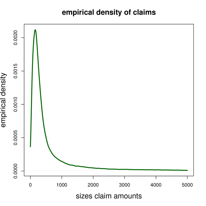
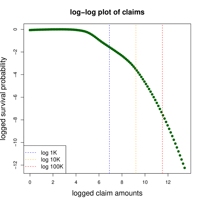
Figure 1: (lhs) Empirical density (upper-truncated at 5,000), (rhs) log-log plot of observed Swiss accident insurance claim amounts.

These claim amounts are supported by 7 features. We have 3 categorical features for the ‘labor sector’ of the injured, the ‘injury type’ and the ‘injured body part’, 1 binary feature telling whether the injury is a ‘work or leisure’ accident, and 3 continuous features corresponding to the ‘age’ of the injured, the ‘reporting delay’ of the claim and the ‘accident quarter’ (capturing seasonality in claims because leisure activities differ in summer and winter times). A preliminary analysis shows that all these features have predictive power, i.e., they are explaining systematic effects in the claim amounts.

For our analysis, we partition the entire data into learning data ${\cal L}=(Y_{i},\boldsymbol{x}_{i})_{1\leq i\leq n}$ that is used for model fitting, and test data ${\cal T}=(Y^{\dagger}_{t},\boldsymbol{x}^{\dagger}_{t})_{1\leq t\leq T}$ which we (only) use for an out-of-sample analysis. We do this partition stratified w.r.t. the claim amounts and in a ratio of $9:1$. This results in learning data ${\cal L}$ of size $n=241,193$ and in test data ${\cal T}$ of size $T=26,799$. We hold on to the same partition in all examples studied. For network fitting we further partition the learning data ${\cal L}=(Y_{i},\boldsymbol{x}_{i})_{1\leq i\leq n}$ into training data ${\cal U}$ and validation data ${\cal V}$. Thus, ${\cal U}\cup{\cal V}$ and ${\cal T}$ are disjoint (and assumed to be independent) so that we can perform a proper out-of-sample forecast evaluation. For a detailed discussion of such a partition of the data for SGD fitting we refer to Section 7.2.3 and, in particular, to Figure 7.7 in Wüthrich–Merz [39].

4.2 Example: deep multiple quantile regression

We apply the framework of Section 3.3 to perform a deep multiple quantile regression. We choose 3 probability levels $0<\tau_{1}<\tau_{2}<\tau_{3}<1$ that we simultaneously estimate; the specific choices considered are $(\tau_{1},\tau_{2},\tau_{3})=(10\%,50\%,90\%)$.

We first discuss pre-processing of feature components before choosing the deep FN network architecture $\boldsymbol{z}^{(d:1)}$. For the 3 categorical variables we use embedding layers of dimension 2, i.e., they are treated by a contextualized embedding. Embedding layers are explained in Section 7.4.1 of Wüthrich–Merz [39]. We use the R library keras for our implementation, and these embedding layers are encoded on lines 3-13 of Listing LABEL:QuantAdd in the supplementary material. The binary variable is encoded by 0-1 and the continuous variables are pre-processed by the MinMaxScaler to ensure that they live on the same scale, see formula (7.30) in Wüthrich–Merz [39] for the MinMaxScaler. Based on this feature encoding we use an FN network of depth $d=3$ having input dimension $r_{0}=3\cdot 2+1+3=10$ (for the categorical, binary and continuous feature components). This 10-dimensional variable enters the network on line 15 of Listing LABEL:QuantAdd. For the deep FN network architecture $\boldsymbol{z}^{(d:1)}$ we choose depth $d=3$ with $(r_{1},r_{2},r_{3})=(20,15,10)$ hidden neurons in the hidden layers, and the hyperbolic tangent activation function $\Psi$. This is encoded on lines 16-18 of Listing LABEL:QuantAdd and gives us learned representations $\boldsymbol{z}_{i}=\boldsymbol{z}^{(d:1)}(\boldsymbol{x}_{i})\in{\mathbb{R}}^{r_{d}+1}$ of dimension $r_{d}+1=11$ of features $\boldsymbol{x}_{i}$. We remark that for insurance data of sample size of roughly 100,000 to 500,000 and with 10 to 20 feature components we have had good experiences by an FN network architecture of this complexity, confirmed by the various examples in Wüthrich–Merz [39]. Therefore, we hold on to this choice.

Next we implement an additive structure (3.3) for deep multiple quantile regression

$$\boldsymbol{x}~{}\mapsto~{}\big{(}Q_{\tau_{1}}(\boldsymbol{x}),~{}Q_{\tau_{2}}(\boldsymbol{x}),~{}Q_{\tau_{3}}(\boldsymbol{x})\big{)}^{\top}~{}\in~{}{\mathbb{R}}^{3}_{+}.$$

This requires that we (re-)use learned representations $\boldsymbol{z}_{i}=\boldsymbol{z}^{(d:1)}(\boldsymbol{x}_{i})$ in the last hidden layer three times and the sequence of quantiles should be monotonically increasing in $\tau_{j}$. We choose as link functions $h$ and $h_{+}$ the log-link which provides us with the exponential function for their inverses, and we then model these quantiles recursively to preserve monotonicity. Lines 20-26 of Listing LABEL:QuantAdd give the corresponding R code, and line 28 outputs these ordered quantiles. The multiplicative approach is rather similar, and the corresponding changes in the R code are shown in Listing LABEL:QuantMult in the supplementary material.

This network architecture has $r=834$ network parameters that need to be fitted to the learning data ${\cal L}$. We use pinball losses (2.8) for the probability levels $(\tau_{1},\tau_{2},\tau_{3})=(10\%,50\%,90\%)$; Listing LABEL:QuantFitting in the supplementary material shows the corresponding R code. These pinball losses then enter the compilation of the model on line 8 of Listing LABEL:QuantFitting. Moreover, we use the nadam version of SGD which usually has a good fitting performance. We fit the two architectures (additive and multiplicative) to our learning data ${\cal L}$, using 80% of the learning data ${\cal L}$ as training data ${\cal U}$ and 20% as validation data ${\cal V}$ to explore the early stopping rule to prevent from over-fitting. To reduce the randomness of SGD fitting we repeat this procedure for 20 different starting points of the algorithm, and we calculate the average predictor over these 20 runs. The results are given in Table 1.

	out-of-sample pinball losses
probability levels $\tau_{j}$	$10\%$	$50\%$	$90\%$
additive approach	141.69	622.11	717.33
multiplicative approach	141.60	622.72	716.46

Table 1: Out-of-sample pinball losses $L_{\tau_{j}}$, $\tau_{j}\in\{10\%,50\%,90\%\}$, on the test data ${\cal T}$ of the deep multiple quantile regression using the additive and the multiplicative approaches.

Table 1 shows the average out-of-sample pinball losses $L_{\tau_{j}}$ on the test data ${\cal T}$ of the two approaches, for $\tau_{j}\in\{10\%,50\%,90\%\}$. We note that the figures of the two approaches are very similar, and we cannot give a clear preference to one of the two approaches. We further explore these results.

	out-of-sample coverage ratios
probability levels $\tau_{j}$	$10\%$	$50\%$	$90\%$
additive approach	10.35%	50.56%	90.22%
multiplicative approach	10.39%	50.74%	90.25%

Table 2: Out-of-sample empirical coverage ratios $\widehat{\tau}_{j}$ below the estimated deep quantile estimates $Q_{\tau_{j}}(\boldsymbol{x}^{\dagger}_{t})$ for $\tau_{j}\in\{10\%,50\%,90\%\}$, see (4.1).

Table 2 shows the out-of-sample empirical coverage ratios on test data ${\cal T}$ of the event that the observation $Y_{t}^{\dagger}$ is smaller or equal to the estimated quantile, that is, we evaluate

$$\widehat{\tau}_{j}~{}=~{}\frac{1}{T}\sum_{t=1}^{T}\mathds{1}_{\left\{Y_{t}^{\dagger}\leq Q_{\tau_{j}}(\boldsymbol{x}^{\dagger}_{t})\right\}},$$ (4.1)

where $Q_{\tau_{j}}(\boldsymbol{x}^{\dagger}_{t})$ is the estimated quantile for level $\tau_{j}\in\{10\%,50\%,90\%\}$ (using either the additive or the multiplicative approach) and evaluated in the features $\boldsymbol{x}^{\dagger}_{t}$ of the out-of-sample observations $Y_{t}^{\dagger}$, $1\leq t\leq T$. Table 2 verifies that the fitted deep multiple quantile regression finds the quantiles (on portfolio level) very well because $\widehat{\tau}_{j}\approx\tau_{j}$; we emphasize that these are out-of-sample figures.

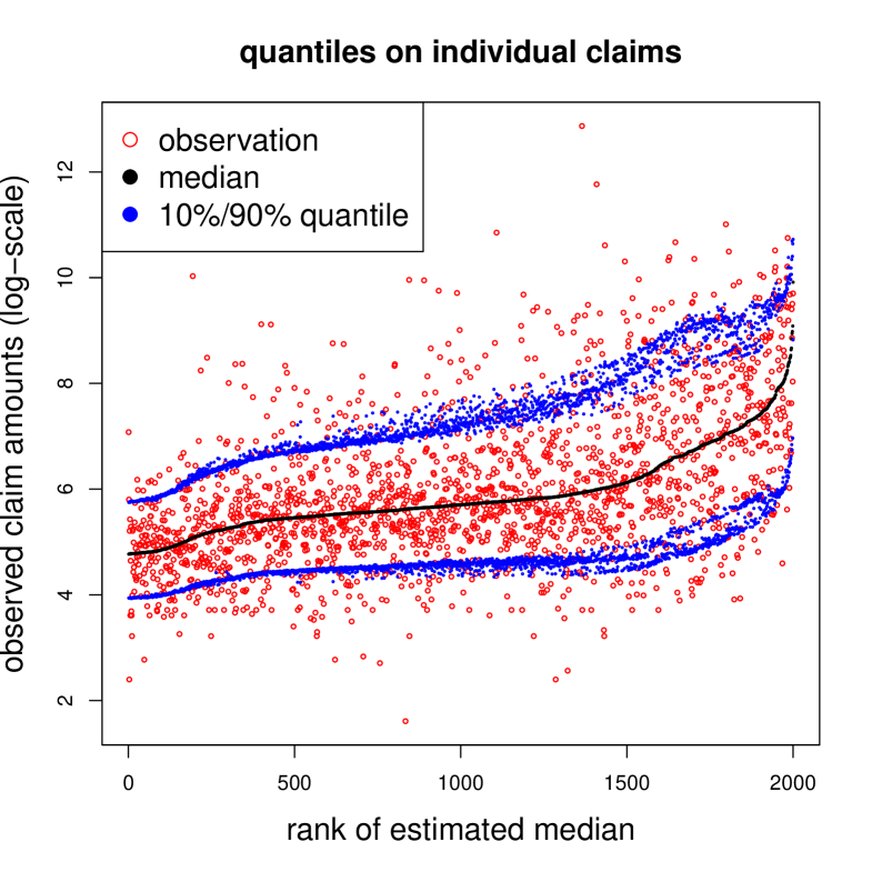
Figure 2: Estimated quantiles $Q_{\tau_{j}}(\boldsymbol{x}^{\dagger}_{t})$ of 2,000 randomly selected individual features $\boldsymbol{x}^{\dagger}_{t}$ on probability levels $\tau_{j}\in\{10\%,50\%,90\%\}$ (blue, black, blue), and the red dots show the corresponding out-of-sample observations (realizations) $Y^{\dagger}_{t}$; the $x$-axis orders the claims w.r.t. the estimated median $Q_{50\%}(\boldsymbol{x}_{t}^{\dagger})$ (in black).

Figure 2 shows the estimated quantiles $Q_{\tau_{j}}(\boldsymbol{x}^{\dagger}_{t})$ for individual features $\boldsymbol{x}^{\dagger}_{t}$ at probability levels $\tau_{j}\in\{10\%,50\%,90\%\}$ (blue, black, blue). The individual observations are ordered w.r.t. the estimated median in black. We observe that this ordering does not imply monotonicity for the other quantiles, especially for bigger claim potentials. This indicates heteroskedasticity in our data. The red dots show the corresponding (out-of-sample) observed claim amounts $Y^{\dagger}_{t}$.

We have analyzed these quantiles also in different granularity, for instance, we have analyzed the empirical coverage ratios on feature levels. Also there the figures look good, but we refrain from giving more plots because we would like to focus on the deep composite model regression proposed in Section 3.3.

4.3 Preliminary considerations for deep composite regression

To fit a deep composite regression model we need a first preliminary step to explore relationship (3.16). This motivates the choices of $\phi$, $\phi_{+}$ and $\phi_{-}$ in (2.16)-(2.18); for $g$ we use the identity function $g(y)=y$, giving us the pinball loss. For this preliminary step, we choose exactly the same network architecture (3.3) as for deep quantile regression, the only change is that we replace the pinball loss by a strictly consistent scoring function for the mean functional, see Theorem 2.4. As Bregman divergence we choose the gamma deviance loss, which corresponds to choice $b=0$ in (3.15). We remark that the gamma model is the most popular model for insurance claim size modeling, and it often provides a first reasonable choice for a regression model; this is also the case for this preliminary step.

We fit three networks of depth $d=3$ with $(r_{1},r_{2},r_{3})=(20,15,10)$ neurons and exponential output activation $h^{-1}$ to (a) all learning data ${\cal L}$, (b) the learning data having observations $Y_{i}>Q_{90\%}(\boldsymbol{x}_{i})$, and (c) the learning data having observations $Y_{i}\leq Q_{90\%}(\boldsymbol{x}_{i})$, where $Q_{90\%}(\boldsymbol{x}_{i})$ is the estimated $\tau=90\%$ quantile from the previous example of Section 4.2. This allows us to analyze (3.14) providing a choice for $\phi$, (3.17) giving a choice for $\phi_{+}$, and (3.18) giving a choice for $\phi_{-}$ for a deep composite model regression at probability level $\tau=90\%$.

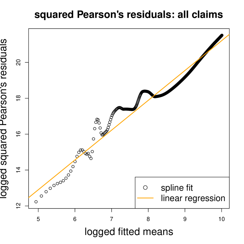
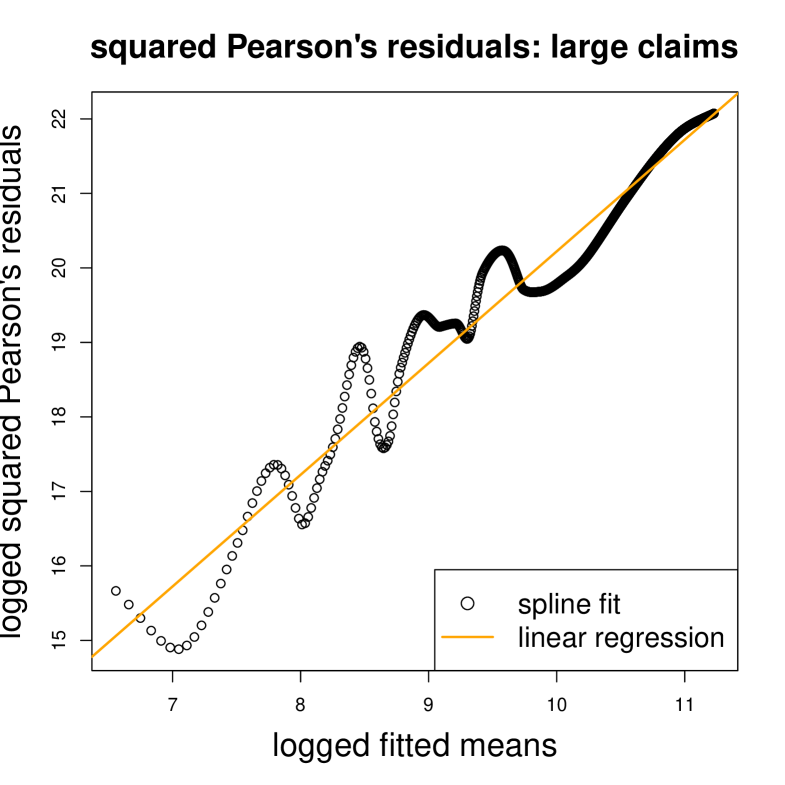
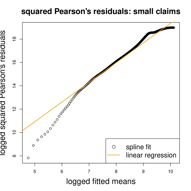
Figure 3: Spline fit and linear regression to the estimated squared Pearson’s residuals as a function of the estimated means (both axis are on the log-scale): (lhs) all claims, (middle) large claims above the 90%-quantile, and (rhs) small claims below the 90%-quantile.

Figure 3 shows a spline fit and a linear regression to the estimated squared Pearson’s residuals $(Y_{i}-\widehat{\mu}(\boldsymbol{x}_{i}))^{2}$, where $\widehat{\mu}(\cdot)$ is the estimated mean functional and where both axis are on the log-scale. The left-hand side shows all claims, the middle shows the situation where we only fit the network to the claims above the estimated quantile $Q_{90\%}(\boldsymbol{x}_{i})$, and the right-hand side only considers the claims below that quantile.

	all claims	large claims	small claims
	$\phi$	$\phi_{+}$	$\phi_{-}$
intercept $\log(c/2)$	4.592	5.229	2.483
slope $2-b$	1.662	1.499	1.687
parameter $b$	0.338	0.401	0.313

Table 3: Linear regression parameters for $c\phi_{b}(\cdot)/2$ from Figure 3.

Table 3 gives the linear regression estimates for $c$ and $b$ in (3.16) for the three cases. We observe that in all three cases we receive $b<1$ which results in derivatives $\phi^{\prime}_{b}(y)=y^{b-1}/(b-1)<0$. This implies that we can only work under scoring function (2.3), because $\phi_{-}$ requires $b>1$, e.g., the square loss function with $b=2$ would work for $\phi_{-}$ but this will not provide optimal convergence rates according to (3.18).

4.4 Deep composite model regression

We are now ready to fit the deep composite regression model for the claims $Y$ w.r.t. the probability level $\tau=90\%$. To this end, we implement the regression function (3.4) and as deep FN network we use the same architecture as in the additive deep multiple quantile regression approach. This regression model is then fitted under the strictly consistent scoring function (2.3) for the joint $\tau$-quantile and lower and upper ES (using the parameters of Table 3).

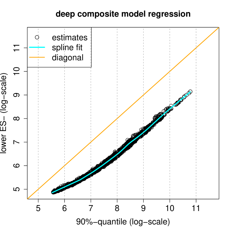
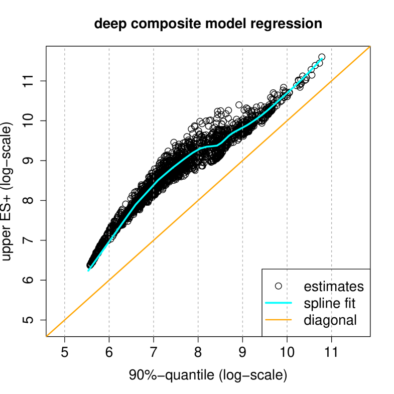
Figure 4: (lhs) Estimated lower $E^{-}_{90\%}(\boldsymbol{x}_{t}^{\dagger})$ vs. estimated quantile $Q_{90\%}(\boldsymbol{x}_{t}^{\dagger})$ and (rhs) estimated upper $E^{+}_{90\%}(\boldsymbol{x}_{t}^{\dagger})$ vs. estimated quantile $Q_{90\%}(\boldsymbol{x}_{t}^{\dagger})$ at probability level $\tau=90\%$.

We fit this network under scoring function (2.3), which is encoded in Listing LABEL:CompositeFitting, using the nadam version of SGD. Figure 4 shows the out-of-sample estimated lower ES, $E^{-}_{90\%}(\boldsymbol{x}_{t}^{\dagger})$, and upper ES, $E^{+}_{90\%}(\boldsymbol{x}_{t}^{\dagger})$, against the estimated quantiles, $Q_{90\%}(\boldsymbol{x}_{t}^{\dagger})$, of 2,000 randomly selected instances $\boldsymbol{x}_{t}^{\dagger}$, and the cyan lines present spline fits to all out-of-sample instances. Basically, the gaps between the cyan lines and the diagonal orange line describe the differences between the ES and the quantile. This gap is of constant size between the lower ES and the quantile above 7 (on the log-scale) which means that the lower ES is a fixed ratio of the quantile. The structure of the upper ES relative to the quantile is more complicated as the gap is becoming smaller with bigger values for the 90% quantile.

Based on these estimates we can now determine the expected value of $Y$, given $\boldsymbol{x}$,

$$\widehat{\mu}(\boldsymbol{x})=\tau\widehat{\rm ES}^{-}_{\tau}(Y|\boldsymbol{x})+(1-\tau)\widehat{\rm ES}^{+}_{\tau}(Y|\boldsymbol{x}).$$

We compare these estimated means to the ones obtained from the (plain vanilla) deep gamma model used in the preparatory Section 4.3; note that the minimization of the gamma deviance loss with $b=0$ in (3.15) is equivalent to the maximization of the log-likelihood function of the gamma distribution.

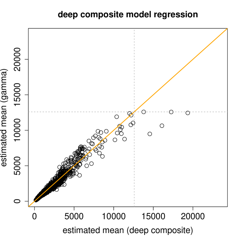
Figure 5: Comparison of estimated out-of-sample means in (lhs) the deep gamma model and the deep composite model, and (rhs) the deep composite model 2 and the deep composite model.

Figure 5 (lhs) compares the deep gamma model to the fitted deep composite model. For small estimated means $\mu(\boldsymbol{x})$ the deep gamma and the deep composite model are rather similar, however, for large estimated means the deep gamma model provides clearly smaller estimates, see gray dotted lines in Figure 5 (lhs). It seems that the deep gamma model under-estimates claims with large expected payments. To verify this, and to check the robustness of the results, we fit a second deep composite model to the data. To this end, we choose a different strictly consistent scoring function, namely, we choose (2.3) which separates small and large claims in an additive way through $\phi_{-}$ and $\phi_{+}$. For the main body of the claims (below the 90%-quantile) we choose the square loss function for $\phi_{-}$ (which corresponds to choice $b=2$ in (3.15)), and for the claims above the probability level we choose $b=0$ for $\phi_{+}$ in (3.15), which corresponds to the gamma deviance loss. We call this second model ‘deep composite model 2’.

Figure 5 (rhs) compares the two fitted deep composite models, using different score functions $L$, which implicitly implies different distributional assumptions in an MLE context. We observe that under both score functions we receive rather similar results, which verifies the robustness of the fittings. There are differences because SGD fitting with early stopping typically finds different ‘good’ solutions, and this inherent fluctuation in SGD can only be reduced by averaging (blending) over model calibrations.

	coverage	lower ES	upper ES
	ratio	identification	identification
	$\widehat{\tau}=90\%$	$\widehat{v}_{-}$	$\widehat{v}_{+}$
deep composite model	90.13%	1.3	-170.7
deep composite model 2	90.10%	-16.5	-203.9
deep gamma model	93.63%	5,612.7	-7,962.4

Table 4: Out-of-sample empirical coverage ratios $\widehat{\tau}$ and identification functions $\widehat{v}_{-}$ and $\widehat{v}_{+}$ of the three considered models.

Analogously to checking the empirical out-of-sample coverage ratios in Table 2, which validated the calibration of our deep quantile models, we now check calibration for the composite triplet consisting of the quantile, the lower ES and the upper ES. For the calibration of $Q_{90\%}$ we again use the empirical coverage defined in (4.1), which should be close to $90\%$. Unfortunately, the lower and the upper ES not only fail to be elicitable, but also turn out not to be identifiable; see Supplement A.1 for a brief discussion of identifiability. Hence, we cannot check the calibration of the models $E_{90\%}^{-}$ and $E_{90\%}^{+}$ standalone, but we can only evaluate the goodness-of-fit of these models jointly with the corresponding quantile model $Q_{90\%}$. The corresponding joint strict identification functions are given as the first and third component in (A.2). The empirical out-of-sample identification functions are

$$\widehat{v}_{-} =\frac{1}{T}\sum_{t=1}^{T}\left[E^{-}_{90\%}(x_{t}^{\dagger})-\frac{Y_{t}^{\dagger}}{0.9}\mathds{1}_{\{Y_{t}^{\dagger}\leq Q_{90\%}(\boldsymbol{x}_{t}^{\dagger})\}}+\frac{Q_{90\%}(\boldsymbol{x}_{t}^{\dagger})}{0.9}\Big{(}\mathds{1}_{\{Y_{t}^{\dagger}\leq Q_{90\%}(\boldsymbol{x}_{t}^{\dagger})\}}-0.9\Big{)}\right],$$ (4.2)

$$\widehat{v}_{+} =\frac{1}{T}\sum_{t=1}^{T}\left[E^{+}_{90\%}(x_{t}^{\dagger})-\frac{Y_{t}^{\dagger}}{0.1}\mathds{1}_{\{Y_{t}^{\dagger}>Q_{90\%}(\boldsymbol{x}_{t}^{\dagger})\}}-\frac{Q_{90\%}(\boldsymbol{x}_{t}^{\dagger})}{0.1}\Big{(}0.1-\mathds{1}_{\{Y_{t}^{\dagger}>Q_{90\%}(\boldsymbol{x}_{t}^{\dagger})\}}\Big{)}\right].$$ (4.3)

Values of $\widehat{v}_{-}$ and $\widehat{v}_{+}$ close to 0 indicate well calibrated models for $(E_{90\%}^{-},Q_{90\%})$ and $(E_{90\%}^{+},Q_{90\%})$, respectively.

Table 4 reports the empirical coverage ratios $\widehat{\tau}$, for $\tau=90\%$, along with the empirical identification functions $\widehat{v}_{-}$ and $\widehat{v}_{+}$ for the two deep composite models and for the deep gamma model; having a gamma distributional assumption from the deep gamma approach of Section 4.3 we can also calculate the composite triplet under this gamma model assumption. In Section 4.3 we have fitted the means $\widehat{\mu}(\boldsymbol{x}^{\dagger}_{t})$ under the gamma assumption. Moreover, using these means we can estimate a dispersion parameter. If we use the deviance dispersion estimate we receive in this gamma model a dispersion parameter of $1/\gamma=1.83$. This allows us to calculate the corresponding quantiles and ES in the gamma model. The lower and upper ES in the gamma model are obtained by

$${\mathbb{E}}\left[Y\left|Y\leq\Gamma_{\gamma,\mu}^{-1}(\tau)\right.\right] = \mu\left(\frac{\Gamma_{\gamma+1,\mu}\left(\Gamma_{\gamma,\mu}^{-1}(\tau)\right)}{\tau}\right),$$

$${\mathbb{E}}\left[Y\left|Y>\Gamma_{\gamma,\mu}^{-1}(\tau)\right.\right] = \mu\left(\frac{1-\Gamma_{\gamma+1,\mu}\left(\Gamma_{\gamma,\mu}^{-1}(\tau)\right)}{1-\tau}\right),$$

where $Y\sim\Gamma_{\gamma,\mu}$ denotes the gamma distribution with mean $\mu>0$ and shape parameter $\gamma>0$.

From Table 4 we conclude that the deep composite regression models meet the right coverage ratio of 90% very well, whereas the deep gamma model results in a too high coverage ratio which indicates that the gamma distributional assumption does not match the tail of the observed data. This carries over to the identification functions of the lower and upper ES. The first deep composite model seems to be slightly better calibrated than the second one, which is indicated by values of $\widehat{v}_{-}$ and $\widehat{v}_{+}$ closer to zero for the first model. The deep gamma model exhibits a poor calibration reflected in high absolute values of $\widehat{v}_{-}$ and $\widehat{v}_{+}$.

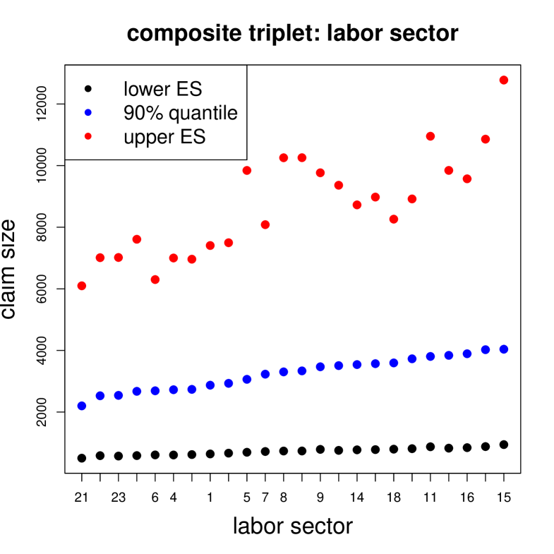
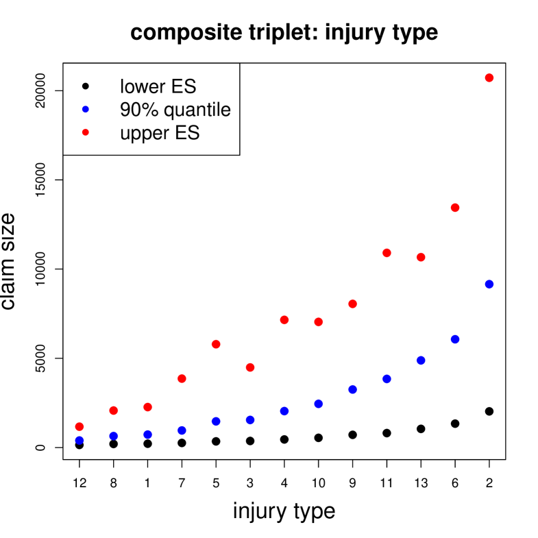
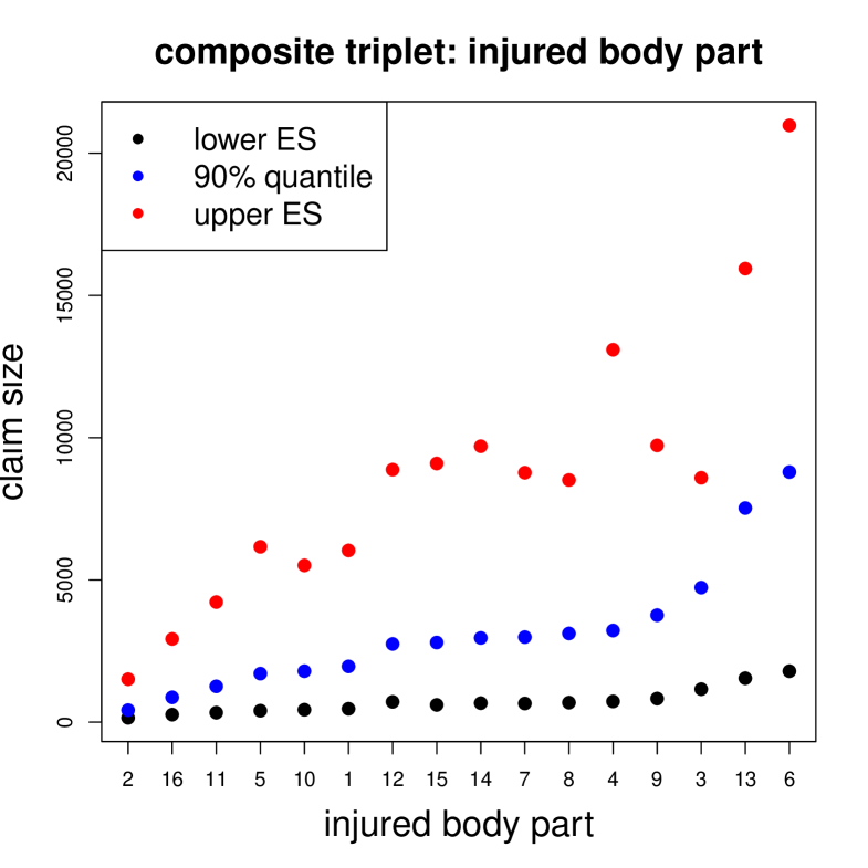
Figure 6: Average marginal estimations for selected feature levels: (lhs) labor sector, (middle) injury type, (rhs) injured body part; ordered on the $x$-axis w.r.t. the average quantile estimates $Q_{90\%}$.

Figure 6 gives marginal estimations of the composite triplet of lower ES, the 90% quantile and the upper ES for the features ‘labor sector’, ‘injury type’ and ‘injured body part’; the $x$-axis is ordered w.r.t. the average 90% quantiles. We observe monotonicity between the average lower ES and the $90\%$ quantiles (black and blue dots), but this monotonicity gets lost w.r.t. the upper ES (red dots). This indicates that we have different regression functions for the main body and the tail of the data. That is, we have developed a very flexible (deep regression) model where features $\boldsymbol{x}\in{\cal X}$ impact predictions differently in the body and the tail of the distributions. This concludes the example.

5 Summary and outlook

We present deep quantile and deep composite model regression. For the composite model, we use a conditional quantile as splicing point, not an absolute threshold. This provides flexibility e.g. in the presence of heteroskedasticity. We utilize a network architecture which respects the natural ordering of quantiles at different probability levels as well as the natural ordering of the composite triplet consisting the the lower expected shortfall, the quantile and the upper expected shortfall at the same probability level. While strictly consistent scoring functions for tuples of quantiles are available, e.g. in the form of sums of pinball losses, and thus M-estimation can be performed for deep quantile models, we first derive and introduce the class of strictly consistent scoring functions for the composite triplet. Addressing the specific choice of the strictly consistent score for the composite triplet, we discuss data-driven choices which potentially increase the efficiency in estimation. The suitability of our methods is illustrated on a real data example with claim amounts describing medical expenses in compulsory Swiss accident insurance.

A relevant extension of our methods is a generalized composite model using two (or even more) splicing points. This allows one to model the influence of features differently for small claim sizes, large claim sizes and the body of the data. This extension seems particularly beneficial since there is empirical evidence that the (conditional) distribution of claim sizes is different in nature for small, claim sizes, the body, and for large claim sizes. Hence, this extension has the potential to increase accuracy of overall claim modeling, which is relevant in insurance pricing. The positive results on the elicitability of the range value at risk (RVaR) – or interquantile expectation – together with the two corresponding quantiles in Fissler–Ziegel [8] suggest the existence of strictly consistent scoring functions for the “extended composite quintuple” consisting of two quantiles (say, the 10% and 90% quantiles) together with the lower ES, upper ES and the range value at risk. However, the specific data-driven choice of the score motivated by efficiency considerations is far from being clear since the class of scoring functions for RVaR and two quantiles is less flexible than the one involving ES and a quantile. E.g. it is shown in [8] that there are no positively homogeneous strictly consistent scores for the former case. Therefore, we defer a detailed study of this extension to future research.

Declaration of competing interest

There is no competing interest.

Appendix A Supplementary material:
Characterisation results on scoring functions

A.1 Identifiability results

Identification functions, also known as moment functions in econometrics, are closely related to scoring functions. Here, the correctly specified functional forecast annihilates the expected identification function rather than minimizing it. Intuitively speaking and subject to smoothness conditions, identification functions can arise as gradients of scoring functions, which explains why their dimension commonly coincides with the dimension of the forecasts.

Definition A.1 (identification function)

Let ${\mathbb{A}}\subseteq{\mathbb{R}}^{k}$. A measurable function $V:{\mathbb{Y}}\times{\mathbb{A}}\to{\mathbb{R}}^{k}$ is a strict ${\mathcal{F}}$-identification function for a given functional $A:{\cal F}\to{\cal P}({\mathbb{A}})$ if ${\mathbb{E}}_{F}\left[|V_{m}(Y;a)|\right]<\infty$ for all $m\in\{1,\ldots,k\}$, for all $Y\sim F\in{\cal F}$ and for all $a\in{\mathbb{A}}$, and if

$${\mathbb{E}}_{F}\left[V(Y;a)\right]=0\quad\Longleftrightarrow\quad a\in A(F),$$ (A.1)

for all $Y\sim F\in{\cal F}$ and for all $a\in{\mathbb{A}}$.

In estimation contexts, identification functions can be used for $Z$-estimation or the (generalized) method of moments [17, 24] as well as for forecast validation or calibration tests as detailed in [25].

Let ${\mathcal{F}}_{\rm cont}^{\tau}$ be the class of distribution functions on ${\mathbb{R}}$ which are continuously differentiable and whose $\tau$-quantiles are singletons. Lemma 2.7 yields the following ‘natural’ strict ${\mathcal{F}}_{\rm cont}^{\tau}$-identification function for $(\mathrm{ES}_{\tau}^{-},q_{\tau},\mathrm{ES}_{\tau}^{+})$

$$V(y;e^{-},v,e^{+})=\begin{pmatrix}e^{-}+\tfrac{1}{\tau}S_{\tau}^{-}(y;v)\\ \mathds{1}_{\{y\leq v\}}-\tau\\ e^{+}-\tfrac{1}{1-\tau}S_{\tau}^{+}(y;v)\end{pmatrix}.$$ (A.2)

Clearly, a linear transformation of full rank of a strict identification function is again a strict identification function (and according to [4, Theorem S.1] there are no further choices, subject to regularity conditions). Therefore, another natural alternative is

$$\widetilde{V}(y;e^{-},v,e^{+})=\begin{pmatrix}\tau e^{-}+(1-\tau)e^{+}-y\\ \mathds{1}_{\{y\leq v\}}-\tau\\ e^{+}-\tfrac{1}{1-\tau}S_{\tau}^{+}(y;v)\end{pmatrix}=\begin{pmatrix}\tau&0&(1-\tau)\\ 0&1&0\\ 0&0&1\end{pmatrix}V(y;e^{-},v,e^{+}).$$ (A.3)

A.2 Assumptions

The proof of Theorem 2.9 exploits Osband’s principle in its form of [6, Theorem 3.2]. Therefore, it uses a similar set of assumptions, which are also in corresponding results such as [8, Theorem 3.7]. More details about their implications and interpretations can be found in [6]. In the sequel, we use the following shorthand notations

$$\bar{L}(F;a):={\mathbb{E}}_{F}[L(Y;a)],\qquad\bar{V}(F;a):={\mathbb{E}}_{F}[V(Y;a)].$$

Assumption A.2

${\mathcal{F}}$ is convex and for every $a\in\operatorname{int}({\mathbb{A}})$, the interior of ${\mathbb{A}}$, there are $F_{1},\ldots,F_{4}\in{\mathcal{F}}$ such that $0\in\operatorname{int}\left(\operatorname{conv}\left(\left\{\bar{V}(F_{1};a),\ldots,\bar{V}(F_{4};a)\right\}\right)\right)\,.$

Since $V$ is a strict ${\mathcal{F}}$-identification function for $(\mathrm{ES}_{\tau}^{-},q_{\tau},\mathrm{ES}_{\tau}^{+})$, Assumption A.2 implies that $(\mathrm{ES}_{\tau}^{-},q_{\tau},\mathrm{ES}_{\tau}^{+})$ maps ${\mathcal{F}}$ surjectively to $\operatorname{int}({\mathbb{A}})$.

Assumption A.3

For all $v_{0}\in\{v\in{\mathbb{R}}:\text{there is }(e^{-},e^{+})\in{\mathbb{R}}^{2}\text{ such that }\ (e^{-},v,e^{+})\in{\mathbb{A}}\}$ there are $F_{1},F_{2}\in{\mathcal{F}}$ with derivatives $f_{1},f_{2}$ such that $q_{\tau}(F_{1})=q_{\tau}(F_{2})=v_{0}$ and $f_{1}(v)\neq f_{2}(v)$.

Assumption A.4

For every $y\in{\mathbb{R}}$ there exists a sequence $(F_{n})_{n\in\mathbb{N}}$ of distributions $F_{n}\in{\mathcal{F}}$ that converges weakly to the Dirac-measure $\delta_{y}$ such that the support of $F_{n}$ is contained in a compact set $K$ for all $n$.

Assumption A.5

$L$ is locally bounded and the complement of the set

$$C:=\{(y;a)\in{\mathbb{R}}\times{\mathbb{A}}\;|\;\text{$L(\cdot;a)$ is continuous at the point $y$}\}$$

has $4$-dimensional Lebesgue measure zero.

Assumption A.6

For every $F\in{\mathcal{F}}$, the function $\bar{L}(F;\cdot)$ is twice continuously differentiable.

A.3 Proof of Theorem 2.9

The proof exploits Osband’s principle [6, Theorem 3.2]. We use the identification function $V$ given in (A.2) rather than the one in (A.3) since this choice is symmetric in the lower and upper ES arguments. Let $F\in{\mathcal{F}}$ with continuous derivative $f$ (which then coincides with one version of the Lebesgue density of $F$). We obtain

$$\bar{V}_{1}(F;e^{-},v,e^{-}) =e^{-}+\tfrac{1}{\tau}(F(v)-\tau)v-\tfrac{1}{\tau}\int_{-\infty}^{v}yf(y)\mathrm{d}y,$$

$$\bar{V}_{2}(F;e^{-},v,e^{-}) =F(v)-\tau,$$

$$\bar{V}_{3}(F;e^{-},v,e^{-}) =e^{+}-\tfrac{1}{1-\tau}(F(v)-\tau)v+\tfrac{1}{1-\tau}\int_{v}^{\infty}yf(y)\mathrm{d}y.$$

The non-vanishing partial derivatives of $\bar{V}(F;\cdot)$ are

$$\partial_{e^{-}}\bar{V}_{1}(F;e^{-},v,e^{-}) =1,$$

$$\partial_{v}\bar{V}_{1}(F;e^{-},v,e^{-}) =\tfrac{1}{\tau}(F(v)-\tau),$$

$$\partial_{v}\bar{V}_{2}(F;e^{-},v,e^{-}) =f(v),$$

$$\partial_{v}\bar{V}_{3}(F;e^{-},v,e^{-}) =-\tfrac{1}{1-\tau}(F(v)-\tau),$$

$$\partial_{e^{+}}\bar{V}_{3}(F;e^{-},v,e^{-}) =1.$$

Osband’s principle [6, Theorem 3.2] yields that, under Assumptions A.2 and A.6, there are continuously differentiable functions $h_{ij}\colon\operatorname{int}({\mathbb{A}})\to{\mathbb{R}}$, $i,j=1,2,3$, such that for all $F\in{\mathcal{F}}$ and all $(e^{-},v,e^{+})\in\operatorname{int}({\mathbb{A}})$

$$\partial_{m}\bar{L}(F;e^{-},v,e^{+})=\sum_{i=1}^{3}h_{mi}(e^{-},v,e^{+})\bar{V}_{i}(F;e^{-},v,e^{+}).$$

Due to Assumption A.6 the Hessian of $\bar{L}(F;\cdot)$ must be symmetric for any $F\in{\mathcal{F}}$. This gives us three conditions which provide a lot of information about the matrix $h=(h_{ij})$. For a given distribution $F\in{\mathcal{F}}$ we shall evaluate these symmetry conditions at the true functional value $(e^{-},v,e^{+})=(\mathrm{ES}_{\tau}^{-}(F),q_{\tau}(F),\mathrm{ES}_{\tau}^{+}(F))$ as well as at an arbitrary value in $\operatorname{int}({\mathbb{A}})$.

Exploiting that the expected identification function vanishes at the true functional value, we obtain for $\partial_{e^{+}}\partial_{e^{-}}\bar{L}(F,e^{-},v,e^{+})=\partial_{e^{-}}\partial_{e^{+}}\bar{L}(F,e^{-},v,e^{+})$ at $(e^{-},v,e^{+})=(\mathrm{ES}_{\tau}^{-}(F),q_{\tau}(F),\mathrm{ES}_{\tau}^{+}(F))$

$$h_{13}(e^{-},v,e^{+})=h_{31}(e^{-},v,e^{+}).$$

Since we can repeat this argument for any distribution $F\in\mathcal{F}$ and by exploiting the surjectivity condition, we get

$$h_{13}\equiv h_{31}.$$ (A.4)

Considering $\partial_{v}\partial_{e^{-}}\bar{L}(F,e^{-},v,e^{+})=\partial_{e^{-}}\partial_{v}\bar{L}(F,e^{-},v,e^{+})$ at $(e^{-},v,e^{+})=(\mathrm{ES}_{\tau}^{-}(F),q_{\tau}(F),\mathrm{ES}_{\tau}^{+}(F))$ we get

$$h_{12}(e^{-},v,e^{+})f(v)=h_{21}(e^{-},v,e^{+}).$$

Assumption A.3 together with a surjectivity argument yields

$$h_{12}\equiv h_{21}\equiv 0.$$

With similar arguments, we get

$$h_{32}\equiv h_{23}\equiv 0.$$

For $F_{1}\in{\mathcal{F}}$ the condition $\partial_{v}\partial_{e^{-}}\bar{L}(F_{1};\cdot)=\partial_{e^{-}}\partial_{v}\bar{L}(F_{1};\cdot)$ evaluated for a general point $(e^{-},v,e^{+})$ implies that

$$0 =\partial_{v}h_{11}(e^{-},v,e^{+})\bar{V}_{1}(F_{1};e^{-},v,e^{+})$$

$$+\big{[}\tfrac{1}{\tau}h_{11}(e^{-},v,e^{+})-\tfrac{1}{1-\tau}h_{13}(e^{-},v,e^{+})-\partial_{e^{-}}h_{22}(e^{-},v,e^{+})\big{]}\bar{V}_{2}(F_{1};e^{-},v,e^{+})$$

$$+\partial_{v}h_{13}(e^{-},v,e^{+})V_{3}(F_{1};e^{-},v,e^{+}).$$

Assumption A.2 implies that there are $F_{2},F_{3}\in{\mathcal{F}}$ such that $\bar{V}(F_{i};e^{-},v,e^{+})$, $i=1,2,3$, are linearly independent. Exploiting the surjectivity once again therefore yields

$$\partial_{v}h_{11}\equiv 0,\qquad\tfrac{1}{\tau}h_{11}-\tfrac{1}{1-\tau}h_{13}\equiv\partial_{e^{-}}h_{22},\qquad\partial_{v}h_{13}\equiv 0.$$ (A.5)

Similarly, the condition $\partial_{v}\partial_{e^{+}}\bar{L}(F;\cdot)=\partial_{e^{+}}\partial_{v}\bar{L}(F;\cdot)$ implies that

$$\partial_{v}h_{31}\equiv 0,\qquad\tfrac{1}{\tau}h_{31}-\tfrac{1}{1-\tau}h_{33}\equiv\partial_{e^{+}}h_{22},\qquad\partial_{v}h_{33}\equiv 0.$$ (A.6)

The third symmetry condition and a repetition of the same arguments finally yields

$$\partial_{e^{+}}h_{11}\equiv\partial_{e^{-}}h_{31},\qquad\partial_{e^{-}}h_{33}\equiv\partial_{e^{+}}h_{31}.$$ (A.7)

Equations (A.5) and (A.6) yield that the functions $h_{11},h_{33},\partial_{e^{-}}h_{22},\partial_{e^{+}}h_{22}$ only depend on $(e^{-},e^{+})$ and are independent of $v$. Equations (A.4) and (A.7) yield that there is a thrice continuously differentiable function $\Phi$ in $(e^{-},e^{+})$ with Hessian $(h_{ij})_{i,j=1,3}$. Moreover, equations (A.5) and (A.6) imply that there is a function $\eta$ in $v$ such that

$$h_{22}(e^{-},v,e^{+})=\eta(v)+\tfrac{1}{\tau}\partial_{e^{-}}\Phi(e^{-},e^{+})-\tfrac{1}{1-\tau}\partial_{e^{+}}\Phi(e^{-},e^{+}).$$

Due to the strict consistency of $L$, the Hessian of its expectation needs to be positive semi-definite at $(e^{-},v,e^{+})=(\mathrm{ES}_{\tau}^{-}(F),q_{\tau}(F),\mathrm{ES}_{\tau}^{+}(F))$. This yields that the submatrix $(h_{ij})_{i,j=1,3}$ is positive semi-definite and that $h_{22}\geq 0$.

Finally, an application of [7, Proposition 1] yields the claim, noting that $\operatorname{int}({\mathbb{A}})$ is simply connected due to the mixture-continuity of $(\mathrm{ES}_{\tau}^{-},q_{\tau},\mathrm{ES}_{\tau}^{+})$ and Assumption A.2. Note that $g^{\prime}=\eta$ and that the Hessian of $\Phi$ is $(h_{ij})_{i,j=1,3}$. $\square$

Appendix B Supplementary material: R code

Listing 1: Deep multiple quantile regression: additive approach.

⬇

1Design <- layer_input(shape = c(4), dtype = ’float32’)

2#

3Cat1 <- layer_input(shape = c(1), dtype = ’int32’)

4Cat1Emb = Cat1 %>%

5 layer_embedding(input_dim=24, output_dim=2, input_length=1) %>% layer_flatten()

6#

7Cat2 <- layer_input(shape = c(1), dtype = ’int32’)

8Cat2Emb = Cat2 %>%

9 layer_embedding(input_dim=13, output_dim=2, input_length=1) %>% layer_flatten()

10#

11Cat3 <- layer_input(shape = c(1), dtype = ’int32’)

12Cat3Emb = Cat3 %>%

13 layer_embedding(input_dim=16, output_dim=2, input_length=1) %>% layer_flatten()

14#

15Network = list(Design, Cat1Emb, Cat2Emb, Cat3Emb) %>% layer_concatenate() %>%

16 layer_dense(units=20, activation=’tanh’, name=’FNLayer1’) %>%

17 layer_dense(units=15, activation=’tanh’, name=’FNLayer2’) %>%

18 layer_dense(units=10, activation=’tanh’, name=’FNLayer3’)

19#

20Q1 <- Network %>% layer_dense(units=1, activation=’exponential’)

21#

22Q20 <- Network %>% layer_dense(units=1, activation=’exponential’)

23Q2 <- list(Q1,Q20) %>% layer_add()

24#

25Q30 <- Network %>% layer_dense(units=1, activation=’exponential’)

26Q3 <- list(Q2,Q30) %>% layer_add()

27#

28model <- keras_model(inputs = list(Design), outputs = c(Q1,Q2,Q3))

Listing 2: Deep multiple quantile regression: multiplicative approach.

⬇

1Q3 <- Network %>% layer_dense(units=1, activation=’exponential’)

2#

3Q20 <- Network %>% layer_dense(units=1, activation=’sigmoid’)

4Q2 <- list(Q3,Q20) %>% layer_multiply()

5#

6Q10 <- Network %>% layer_dense(units=1, activation=’sigmoid’)

7Q1 <- list(Q2,Q10) %>% layer_multiply()

Listing 3: Fitting a deep multiple quantile regression with pinball losses.

⬇

1PinB1 <- function(y_true, y_pred){k_mean(k_maximum(y_true - y_pred, 0) * 0.1

2 + k_maximum(y_pred - y_true, 0) * (1 - 0.1))}

3PinB2 <- function(y_true, y_pred){k_mean(k_maximum(y_true - y_pred, 0) * 0.5

4 + k_maximum(y_pred - y_true, 0) * (1 - 0.5))}

5PinB3 <- function(y_true, y_pred){k_mean(k_maximum(y_true - y_pred, 0) * 0.9

6 + k_maximum(y_pred - y_true, 0) * (1 - 0.9))}

7#

8model %>% compile(loss = list(PinB1, PinB2, PinB3), optimizer = ’nadam’)

Listing 4: Fitting a deep composite model regression with scoring function (2.3).

⬇

1Loss <- function(y_true, y_pred){

2 mu <- tau0 * y_pred[,1] + (1-tau0) * y_pred[,3]

3 k_mean(

4 (k_maximum(y_true[,1] - y_pred[,2], 0) * 0.9 +

5 k_maximum(y_pred[,2]- y_true[,1], 0) * 0.1)*

6 (1 - c2 * y_pred[,3]^(b2-1) / ((b2-1) * 0.1)) +

7 c2/(b2-1) * (y_pred[,3]^(b2-1)*(y_pred[,3]-y_true[,1])

8 -y_pred[,3]^b2/b2+y_true[,1]^b2/b2)+

9 c1/(b1-1) * (mu^(b1-1)*(mu_true[,1])-mu^b1/b1+y_true[,1]^b1/b1)) }

10#

11model %>% compile(loss = Loss, optimizer = ’nadam’)

References

- [1] Barendse, S. (2020). Efficiently weighted estimation of tail and interquartile expectations. SSRN Manuscript ID 2937665.
- [2] Cooray, K., Ananda, M.M.A. (2005). Modeling actuarial data with composite lognormal-Pareto model. Scandinavian Actuarial Journal 2005/5, 321–334.
- [3] Dimitriadis, T., Bayer, S. (2019). A joint quantile and expected shortfall regression framework. Electronic Journal of Statistics 13/1, 1823–1871.
- [4] Dimitriadis, T., Fissler, T., Ziegel, J.F. (2020). The efficiency gap. arXiv, 2010.14146.
- [5] Embrechts, P., Wang, R. (2015). Seven proofs for the subadditivity of expected shortfall. Dependence Modeling 3, 126–140.
- [6] Fissler, T., Ziegel, J.F. (2016). Higher order elicitability and Osband’s principle. The Annals of Statistics 44/4, 1680–1707.
- [7] Fissler, T., Ziegel, J.F. (2021). Correction note: Higher order elicitability and Osband’s principle. The Annals of Statistics 49/1, 614.
- [8] Fissler, T., Ziegel, J.F. (2021). On the elicitability of range value at risk. Statistics & Risk Modeling 38/1–2, 25–46.
- [9] Frongillo, R., Kash, I. (2021). Elicitation complexity of statistical properties. Biometrika 108/4, 857–879.
- [10] Fung, T.C., Badescu, A.L., Lin, X.S. (2021). A new class of severity regression models with an application to IBNR prediction. North American Actuarial Journal 25/2, 206–231.
- [11] Gan, G., Valdez, E.A. (2018). Fat-tailed regression modeling with spliced distributions. North American Actuarial Journal 22/4, 554–573.
- [12] Gneiting, T. (2011). Making and evaluating point forecasts. Journal of the American Statistical Association 106/494, 746–762.
- [13] Gneiting, T. (2011). Quantiles as optimal point forecasts. International Journal of Forecasting, 27/2, 197–207.
- [14] Gneiting, T., Raftery, A.E. (2007). Strictly proper scoring rules, prediction, and estimation. Journal of the American Statistical Association 102/477, 359–378.
- [15] Grün, B., Miljkovic, T. (2019). Extending composite loss models using a general framework of advanced computational tools. Scandinavian Actuarial Journal 2019/8, 642–660.
- [16] Guillen, M., Bermúdez, L., Pitarque, A., (2021). Joint generalized quantile and conditional tail expectation for insurance risk analysis. Insurance: Mathematics and Economics 99, 1–8.
- [17] Hansen, L.P. (1982). Large sample properties of generalized method of moments estimators. Econometrica 50/4, 1029–54.
- [18] Hastie, T., Tibshirani, R., Friedman, J. (2009). The Elements of Statistical Learning. Data Mining, Inference, and Prediction. 2nd edition. Springer Series in Statistics.
- [19] Jørgensen, B. (1987). Exponential dispersion models. Journal of the Royal Statistical Society, Series B 49/2, 127–145.
- [20] Koenker, R., Bassett, G., Jr. (1978). Regression quantiles. Econometrica 46/1, 33–50.
- [21] Laudagé, C., Desmettre, S., Wenzel, J. (2019). Severity modeling of extreme insurance claims for tariffication. Insurance: Mathematics and Economics 88, 77–92.
- [22] McNeil, A.J., Frey, R., Embrechts, P. (2015). Quantitative Risk Management: Concepts, Techniques and Tools. Revised edition. Princeton University Press.
- [23] Meinshausen, N. (2006). Quantile regression forests. Journal of Machine Learning Research 7, 983–999.
- [24] Newey, W.K., McFadden, D. (1994). Large sample estimation and hypothesis testing. In R.F. Engle and D. McFadden (Eds.), Handbook of Econometrics, Volume 4, Chapter 36, Elsevier, 2111–2245.
- [25] Nolde, N., Ziegel, J.F. (2017). Elicitability and backtesting: Perspectives for banking regulation. Annals of Applied Statistics 11/4, 1833–1874.
- [26] Osband, K.H. (1985). Providing Incentives for Better Cost Forecasting. PhD thesis, University of California, Berkeley.
- [27] Parodi, P. (2020). A generalised property exposure rating framework that incorporates scale-independent losses and maximum possible loss uncertainty. ASTIN Bulletin 50/2, 513–553.
- [28] Pigeon, M., Denuit, M.. Composite lognormal-Pareto model with random threshold. Scandinavian Actuarial Journal 2011/3, 177–192.
- [29] Richman, R. (2021). Mind the gap – safely incorporating deep learning models into the actuarial toolkit. SSRN Manuscript ID 3857693.
- [30] Saerens, M. (2000). Building cost functions minimizing to some summary statistics. IEEE Transactions on Neural Networks 11, 1263–1271.
- [31] Savage, L.J. (1971). Elicitable of personal probabilities and expectations. Journal of the American Statistical Association 66/336, 783–810.
- [32] Scollnik, D.P.M. (2007). On composite lognormal-Pareto models. Scandinavian Actuarial Journal 2007/1, 20–33.
- [33] Takeuchi, I., Le, Q.V., Sears, T.D., Smola, A.J. (2006). Nonparametric quantile estimation. Journal of Machine Learning Research 7, 1231–1264.
- [34] Thomson, W. (1979). Eliciting production possibilities from a well-informed manager Journal of Economic Theory 20, 360–380.
- [35] Tweedie, M.C.K. (1984). An index which distinguishes between some important exponential families. In: Statistics: Applications and New Directions. Ghosh, J.K., Roy, J. (Eds.). Proceeding of the Indian Statistical Golden Jubilee International Conference, Indian Statistical Institute, Calcutta, 579–604.
- [36] Uribe, J.M., Guillen, M. (2019). Quantile Regression for Cross-Sectional and Time Series Data Applications in Energy Markets using R. Springer.
- [37] Van der Vaart, A.W. (1998). Asymptotic Statistics. Cambridge University Press.
- [38] Weber, S. (2006). Distribution-invariant risk measures, information, and dynamic consistency. Mathematical Finance 16, 419–441.
- [39] Wüthrich, M.V., Merz, M. (2021). Statistical foundations of actuarial learning and its applications. SSRN Manuscript ID 3822407.