Annealed inhomogeneities in random ferromagnets

Abstract

Abstract

We consider spin models on complex networks frequently used to model social and technological systems. We study the annealed ferromagnetic Ising model for random networks with either independent edges (Erdős-Rényi), or with prescribed degree distributions (configuration model). Contrary to many physical models, the annealed setting is poorly understood and behaves quite differently than the quenched system. In annealed networks with a fluctuating number of edges, the Ising model changes the degree distribution, an aspect previously ignored. For random networks with Poissonian degrees, this gives rise to three distinct annealed critical temperatures depending on the precise model choice, only one of which reproduces the quenched one. In particular, two of these annealed critical temperatures are finite even when the quenched one is infinite, since then the annealed graph creates a giant component for all sufficiently small temperatures. We see that the critical exponents in the configuration model with deterministic degrees are the same as the quenched ones, which are the mean-field exponents if the degree distribution has finite fourth moment, and power-law-dependent critical exponents otherwise. Remarkably, the annealing for the configuration model with random i.i.d. degrees washes away the universality class with power-law critical exponents.

In spin systems with disorder usually two averaging procedure are considered: the quenched state, that is used to model the setting where the couplings between spins are essentially frozen and the annealed state, in which spins and disorder are treated on the same footing. In this paper we ask the following question: how different are the quenched and annealed states of a disordered ferromagnet? Do they share the same critical temperatures and critical exponents? We show here that this seemingly simple question does not admit a simple answer. Instead, the comparison of the annealed state of a random ferromagnet to the quenched one reveals a host of surprises. As we shall see by considering several models of random graphs, the answer depends sensitively on whether the total number of edges of the underlying random graph is fixed, or is allowed to fluctuate. Indeed, the typical graph under the annealed measure re-arranges itself in order to maximize the ferromagnetic alignment of spins by increasing the number of edges. As a consequence, we argue that the annealed critical temperature is highly model-dependent, even in the case of graphs that are asymptotically equivalent (such as the different versions of the simple Erdős-Rényi random graph). This is to be contrasted to the quenched critical temperature that is essentially the same for all locally-tree like graphs.

The difference between quenched and annealed becomes even more substantial in the presence of inhomogeneities that produce a fat-tail degree distribution, whose tail behavior is characterized by a power-law exponent $\tau>2$. In this case it has been shown leone ; doro-zero that quenched models, on top of the mean-field universality class, may have other university classes, where the quenched critical exponents depend on the power-law exponent $\tau$, taking the mean-field values for $\tau>5$, but different values for $\tau\in(3,5)$.

Our analysis shows that the picture radically changes in the annealed setting. In the context of the configuration model we find that when the degrees are fixed, one obtains the same universality classes as in the quenched setting. However the annealed partition function of the configuration model with random (i.i.d.) degrees blows up for fat-tail degree distributions. Furthermore, for models having a well-defined partition function,

the power-law universality classes are washed away,

and only the mean-field universality class survives.

The distinction between quenched and annealed averaging is particularly relevant for social systems, where the network of acquaintances of members of a group changes quite rapidly, on a time scale that is comparable to that of opinion changes bara ; nbw ; decelle . In such settings, the annealed setting is the most appropriate.

The multi-facetted phenomenology that we find in the description of the annealed state did not emerge in previous studies of disordered ferromagnets bianconi ; doro-zero ; GIU1 ; lee ; leone , that instead suggested the annealed state to be described by an approximate mean-field theory that accounts for heterogeneity of the graph (so-called“annealed network approach” doro-zero ). Our analysis shows that this approximate theory may fail to identify the critical temperature, even for very simple random graph models. In the following we first discuss the case of homogeneous models with Poissonian degrees and, afterwards, we extend our analysis to models with inhomogeneities.

Models with Poisson degree distributions. Let us consider the Ising model on a network with $n$ vertices. Given a spin configuration $\sigma=(\sigma_{1},\ldots,\sigma_{n})\in\{-1,+1\}^{n}$ and a random graph with vertex set $V$ and edge set $E$, the Hamiltonian is defined as

$$H_{n}(\sigma)=\beta\sum_{(i,j)\in E}\sigma_{i}\sigma_{j}+B\sum_{i\in V}\sigma_{i}$$ (1)

where $\beta$ is the inverse temperature and $B$ an external field. The order parameter is the spontaneous annealed magnetization $M(\beta)=\lim_{B\to 0^{+}}M(\beta,B),$ where

$$M(\beta,B)=\lim_{n\to\infty}\frac{\Big{\langle}\sum_{\sigma}\Big{(}\frac{1}{n}\sum_{i=1}^{n}\sigma_{i}\Big{)}{\rm e}^{H_{n}(\sigma)}\Big{\rangle}}{\Big{\langle}\sum_{\sigma}{\rm e}^{H_{n}(\sigma)}\Big{\rangle}}\;.$$ (2)

Here $\langle\cdot\rangle$ denotes expectation over the randomness of the graph, which, in the annealed setting, appears both in numerator and denominator.

The simplest possible random network is the binomial Erdős-Rényi, denoted $\text{bER}(\lambda/n)$, in which a pair of vertices in $[n]=\{1,\ldots,n\}$ is connected (independently from other pairs) with the same probability $\lambda/n,\,\lambda>0$. In this case, the Hamiltonian (1) becomes

$$H^{\text{bER}(\lambda/n)}(\sigma)=\beta\sum_{1\leq i<j\leq n}I_{i,j}\sigma_{i}\sigma_{j}+B\sum_{i=1}^{n}\sigma_{i},$$ (3)

where $I_{i,j}$ are independent and identically distributed Bernoulli random variables with $\mathbb{P}(I_{i,j}=1)=\lambda/n$ defining the adjacency matrix of the network. The random variable $D_{i}=\sum_{k}I_{i,k}$, counting the number of edges connected to vertex $i$ is the degree of $i$, which for large $n$ results in a Poisson random variable with parameter $\lambda$. As shown in the Supplementary Material, the annealed magnetization (2) of the binomial Erdős-Rényi model solves the mean-field Curie-Weiss equation with a renormalized temperature $\beta\mapsto\sinh(\beta)$, i.e.,

$$M^{\text{bER}}=\tanh\Big{(}\lambda\sinh(\beta)M^{\text{bER}}+B\Big{)},$$ (4)

yielding a critical inverse temperature

$$\beta_{c}^{\text{bER}}={\rm asinh}(1/\lambda),$$ (5)

and critical exponents of the mean-field universality class.

The “annealed network approach” introduced in bianconi ; doro-zero is based on the idea of replacing the model with Hamiltonian (1) by a mean-field model on a weighted fully connected graph described by the Hamiltonian

$$H^{\mathrm{mf}}(\sigma)=\frac{\beta}{2}\sum_{i,j=1}^{n}\frac{D_{i}D_{j}}{\ell_{n}}\sigma_{i}\sigma_{j}+B\sum_{i=1}^{n}\sigma_{i},$$ (6)

where $\ell_{n}=\sum_{i}D_{i}$. This translates into an equation for the magnetization given by

$$M^{\mathrm{mf}}(\beta,B)=\left\langle\tanh\Big{(}\beta yD+B\Big{)}\right\rangle,$$ (7)

where $y\in(0,1)$ is a solution of the mean-field equation

$$y=\left\langle{D}\tanh\Big{(}\beta yD+B\Big{)}\right\rangle/\big{\langle}D\big{\rangle}\,.$$ (8)

In the case of models with Poissonian degrees with $\big{\langle}D\big{\rangle}=\lambda$, the linearization around $y=0$ yields the inverse critical temperature

$$\beta_{c}^{\mathrm{mf}}=1/(\lambda+1),$$ (9)

and critical exponents are those of the mean-field universality class. Therefore, the “annealed network approach” predicts the correct annealed critical exponents, but fails in determining the critical temperature. As shown in Fig. 1, the discrepancy between the true value of the critical temperature (red curve) and the one predicted by the annealed network approach (blue curve) increases as the average connectivity $\lambda$ is decreased. In particular at $\lambda=0$ one gets $\beta_{c}^{\mathrm{mf}}=1$, which is clearly unphysical.

It is interesting to compare the annealed magnetization (2) to the magnetization that is obtained in the quenched setting GGHP2 . For all the models that are locally tree-like leone ; doro-zero ; dm ; DGGHP , the quenched magnetization $M^{\mathrm{qu}}(\beta,B)$ is

$$M^{\mathrm{qu}}(\beta,B)=\left\langle\frac{{\rm e}^{2B}-\prod_{i=1}^{D}X_{i}}{{\rm e}^{2B}+\prod_{i=1}^{D}X_{i}}\right\rangle,$$ (10)

where $(X_{i})_{i\geq 0}$ are i.i.d. random variables satisfying

$$X_{0}\overset{(\mathcal{L})}{=}\frac{{\rm e}^{-\beta+B}+{\rm e}^{\beta-B}\prod_{i=1}^{D}X_{i}}{{\rm e}^{\beta+B}+{\rm e}^{-\beta-B}\prod_{i=1}^{D}X_{i}}.$$ (11)

The linearization around $X=1$ yields

$$\beta_{c}^{\mathrm{qu}}={\rm atanh\,}\left(1/\lambda\right).$$ (12)

Surprisingly, the quenched critical value coincides with the one that is obtained by solving the annealed Ising model on the combinatorial Erdős-Rényi random graph, denoted $\text{cER}(\lambda n/2)$, with $n$ vertices and a fixed number of edges $\lambda n/2$ placed uniformly at random. The annealed magnetization of the combinatorial Erdős-Rényi random graph satisfies yet another mean-field equation (see Supplementary Material)

$$M^{\text{cER}}=\tanh\Big{[}\frac{\lambda(1-{\rm e}^{-2\beta})M^{\text{cER}}}{2+(1-{\rm e}^{-2\beta})((M^{\text{cER}})^{2}-1)}+B\Big{]}\,.$$ (13)

The linearization around zero gives

$$\beta_{c}^{\text{cER}}=\beta_{c}^{\mathrm{qu}}.$$ (14)

We observe that, although the bER and the cER are asymptotically equivalent random graph models (in particular they both have Poisson degrees), their annealed magnetization satisfies different equations yielding different critical temperatures. We show in the Supplementary Material that this difference arises from the fact that in the cER, the number of edges is fixed, whereas annealing macroscopically increases the number of edges in the bER.

Model with inhomogeneities. We now go to a more general setting that allows to treat inhomogeneities described by general degree distributions (beyond the Poissonian case).

We first consider the configuration model with fixed degrees, denoted by $\mathrm{CM(d)}$ that is obtained by prescribing the degree values $\mathrm{d}=(d_{i})_{i\in{\color[rgb]{0,0,0}[n]}{\color[rgb]{0,0,0}}}$ and connecting the vertices uniformly at random remco . In the Supplementary Material we show that, denoting by $D$ the degree of a uniformly chosen vertex, the annealed magnetization is

$$M^{\mathrm{CM(d)}}(\beta,B)=\left\langle\tanh\Big{(}\beta yD+B\Big{)}\right\rangle,$$ (15)

where $y\in(0,1)$ is a solution to

$$\frac{1-{\rm e}^{-4\beta y}}{1+{\rm e}^{-4\beta y}-2{\rm e}^{-2\beta(1+y)}}=\left\langle D\tanh\Big{(}\beta yD+B\Big{)}\right\rangle/\left\langle D\right\rangle.$$ (16)

Comparing (16) and (8) we see once more that the “annealed network approach” correctly predict a mean-field behaviour for the annealed magnetization, but that the mean-field equation for $y$ is again quite different. From the linearization of equation (16) around $y=0$ one finds that the annealed critical point $\beta_{c}^{\mathrm{CM(d)}}$ of the configuration model with prescribed Poissonian degrees is

$$\beta_{c}^{\mathrm{CM(d)}}=\beta_{c}^{\mathrm{qu}},$$ (17)

which is consistent with the claim that fixing the number of edges recovers the quenched critical temperature.

If instead the configuration model is constructed by considering random i.i.d.  degrees $D_{i}$ (denoted by $\mathrm{CM(D)}$), then the situation drastically changes. The additional randomness of the degrees implies that only degrees distributions with exponential tails are possible. Indeed, by considering the configuration $\sigma$ with all spins up, one immediately obtains the bound

$$\left\langle{\rm e}^{\beta\sum_{i\in V}D_{i}/2}\right\rangle\leq{\rm e}^{-n|B|}\left\langle Z_{n}\right\rangle\leq 2^{n}\left\langle{\rm e}^{\beta\sum_{i\in V}D_{i}/2}\right\rangle\,.$$ (18)

The annealed free energy is thus only well-defined in the thermodynamic limit if $\left\langle{\rm e}^{\beta D/2}\right\rangle<\infty$. Assuming this to be the case, then as shown in the Supplementary Material, the annealed magnetization reads

$$M^{\mathrm{CM(D)}}(\beta,B)=\left\langle\tanh\Big{(}\beta yD_{\beta}+B\Big{)}\right\rangle,$$ (19)

where $y\in(0,1)$ is a solution to

$$\frac{1-{\rm e}^{-4\beta y}}{1+{\rm e}^{-4\beta y}-2{\rm e}^{-2\beta(1+y)}}=\left\langle D_{\beta}\tanh\Big{(}\beta yD_{\beta}+B\Big{)}\right\rangle/\left\langle D_{\beta}\right\rangle.$$ (20)

Here $D_{\beta}$ is the new law that arises from the law of $D$ as a consequence of the randomness of the degrees. Indeed, in the presence of i.i.d. degrees that are copies of a random variable $D$ with distribution ${\bm{p}}=(p_{k})_{k\geq 1}$, i.e. $\mathbb{P}(D=k)=p_{k}$, the annealed ‘pressure’ ($=-f/\beta$ with $f$ the annealed free energy) is C

$$\varphi^{\mathrm{CM(D)}}(\beta,B)=\sup_{{{\bm{q}}}}\left[\varphi^{\mathrm{CM(d)}}(\beta,B;{\bm{q}})-H({\bm{q}}|{\bm{p}})\right],$$ (21)

where $\varphi^{\mathrm{CM(d)}}(\beta,B;{\bm{q}})$ denotes the pressure of the configuration model with a deterministic degree distribution ${\bm{q}}$, and $H({\bm{q}}|{\bm{p}})$ is the relative entropy of ${\bm{q}}$ with respect to ${\bm{p}}$

$$H({\bm{q}}|{\bm{p}})=\sum_{k}{q_{k}}\log{\frac{q_{k}}{p_{k}}}.$$ (22)

The equations (19), (20) are then obtained by deriving w.r.t. the external field $B$. To identify the critical temperature, one takes $B\searrow 0$, in which case the law of $D_{\beta}$ turns out to be a $\beta$-dependent exponential tilting of the degree-distribution $D$,

$$q_{k}(\beta)=p_{k}\cosh(\beta)^{k/2}/c(\beta),$$ (23)

with $c(\beta)=\left\langle\cosh(\beta)^{D/2}\right\rangle.$ Thus, since $\cosh(\beta)>1$, under the annealed measure of the configuration model, the typical graph in the case of random i.i.d. degrees re-arranges itself (compared to the case of deterministic degrees) in order to maximize the ferromagnetic alignment of spins, and it does so by increasing the number of edges.

In particular, when the degree $D$ is Poissonian with mean $\lambda$, the tilted degree $D_{\beta}$ is again a a Poisson random variable with mean $\lambda\sqrt{\cosh(\beta)}$. The linearization of (20) around $y=0$ then yields an implicit equation for the critical inverse temperature

$$\beta_{c}={\rm atanh\,}\Big{(}\frac{1}{\lambda\sqrt{\cosh(\beta_{c})}}\Big{)},$$ (24)

whose solution $\beta_{c}^{\mathrm{CM(D)}}$ is

$$-\log(2\lambda^{2})+\log\left[1+\sqrt{1+4\lambda^{4}}+\sqrt{2+2\sqrt{1+4\lambda^{4}}}\right].$$ (25)

Comparing to (17), we see that while the annealed $\mathrm{CM(d)}$ with fixed Poissonian degrees has a phase transition only when a giant connected component exists $(\lambda>1)$, the $\mathrm{CM(D)}$ with random Poissonian degrees has a finite critical temperature for all $\lambda>0$.

In Fig. 1, we collect the results obtained so far. For all the random networks with Poisson degree distribution, the quenched critical temperature is given by (12), but we have 4 different values of the annealed critical temperatures. In particular, the combinatorial Erdős-Rényi (cER) and the configuration model $\mathrm{CM(d)}$, both having a fixed number of edges, reproduce the quenched critical value, whereas the binomial Erdős-Rényi (bER) and the configuration model $\mathrm{CM(D)}$ with a fluctuating number of edges, have a critical value that is model-dependent (and different from that of the mean-field “annealed network approach”).

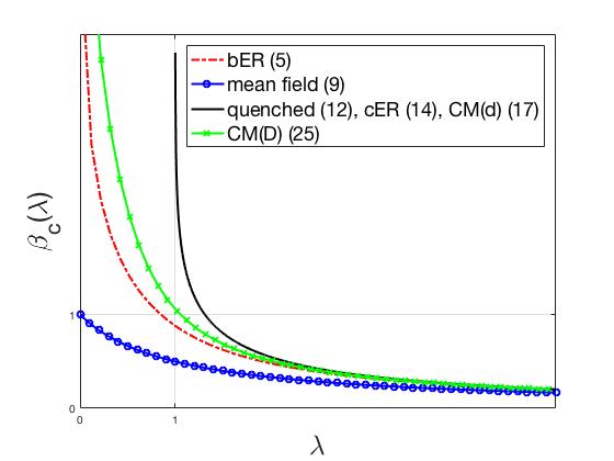
Figure 1: Annealed critical points $\beta_{c}(\lambda)$ for models with degree distribution Poisson($\lambda$). Points are guides to the eye.

Presence or absence of power-law universality class. We now analyze the annealed critical exponents. One immediately sees that for homogeneous networks (i.e., Poissonian degree distribution), the critical exponents are those of the Curie-Weiss model. Therefore, we concentrate on inhomogeneous networks and, for the sake of space, we consider the configuration model.

We start from the case of fixed degrees: by Taylor expansion of Eq. (15), (16), we now obtain a critical temperature $\beta_{c}^{\mathrm{CM(d)}}={\rm atanh\,}\left(\frac{\langle D\rangle}{\langle D(D-1)\rangle}\right)$. Thus the annealed system has a ferromagnetic phase transition when $\langle D^{2}\rangle<\infty$ and is always in the ferromagnetic phase when $\langle D^{2}\rangle=\infty$. As for the critical exponents, we find those of the mean-field universality class, provided that $\langle D^{4}\rangle<\infty$. If this condition is not met, then new universality classes arise leone ; doro-zero ; DGH1 . For instance, for power-law distributed degrees, i.e. $p_{k}\sim k^{-\tau}$ with an exponent $3<\tau<5$, we find

$$\alpha=\frac{5-\tau}{\tau-3},\qquad\beta=\frac{1}{\tau-3},\qquad\gamma=1,\qquad\delta=\tau-2.$$

This scenario of a family of universality classes (labeled by the degree power-law exponent $\tau$) coincides with what was found for all quenched networks with a locally-tree like structure leone ; doro-zero ; DGH1 .

We now move to the configuration model with random i.i.d. degrees. Taylor expansion of (19) and (20) identifies the critical inverse temperature $\beta_{c}^{\mathrm{CM(D)}}$ as the solution of the equation

$$\beta={\rm atanh\,}\left(\frac{\left\langle D_{\beta}\right\rangle}{\left\langle D_{\beta}(D_{\beta}-1)\right\rangle}\right).$$

As we have already remarked, for power-law degrees the free energy simply blows up. Thus, we have to restrict to degree distributions with exponential tails, in which case, the free energy diverges when $\beta$ is large, but not when it is small. In this case, the critical value $\beta_{c}^{\mathrm{CM(D)}}$ is strictly smaller than the value $\beta$ where the free energy explodes. Then, provided that $\left\langle{\rm e}^{\beta_{c}^{\mathrm{CM(D)}}D/2}\right\rangle<\infty$ (cf. (18)), the tilted degree distribution $q(\beta)$ in (23) always has exponential tails, since $\cosh(\beta)<{\rm e}^{\beta}$. Therefore, the empirical degree distribution $q(\beta,B)$ of the random graph under the annealed Ising model with a non-zero field $B$, close to the critical point, has exponential tails. As a result, power-law degree distributions cannot occur, and thus the critical exponents are all equal to those of the Curie-Weiss model. In this case, there exists only one universality class, compared to the several ones for the setting of deterministic degrees.

Acknowledgements. We thank J.F.F. Mendes for useful discussions. RvdH acknowledges financial support from Gravitation-grant NETWORKS-024.002.003.

SUPPLEMENTARY MATERIAL

I Annealed combinatorial Erdős-Rényi

Here, we investigate the annealed Ising model on the Erdős-Rényi random graph $\text{cER}(\lambda n/2)$ of size $n$ with a fixed number $m=\lambda n/2$ of edges placed uniformly at random, for which we prove that the critical value equals the quenched critical value.

Let us denote $Z^{\text{cER}}_{n,+}(k)$ the partition function where we fix $|\sigma_{+}|=k$ with $\sigma_{+}$ the subset of sites with positive spin. Then, recaling the Hamiltonian (3), the annealed partition function equals

$$\left\langle Z^{\text{cER}}_{n}\right\rangle=\left\langle\sum_{\sigma}{\rm e}^{H^{\text{cER}}(\sigma)}\right\rangle=\sum_{k=0}^{n}\left\langle Z^{\text{cER}}_{n,+}(k)\right\rangle.$$ (26)

Using

$$H^{\text{cER}}(\sigma)=m-2e(\sigma_{+},\sigma_{-})+B(2|\sigma_{+}|-n)$$

where $e(\sigma_{+},\sigma_{-})$ is the number of edges connecting $\sigma_{+}$ to $\sigma_{-}$, we get

$$\left\langle Z^{\text{cER}}_{n,+}(k)\right\rangle=\left\langle\sum_{|\sigma_{+}|=k}{\rm e}^{\beta m-2\beta e(\sigma_{+},\sigma_{-})+\beta Bn(2k-1)}\right\rangle.$$ (27)

By adding edges one-by-one, we see that, with $m=\lambda n/2$ and $N=n(n-1)/2$, we get

$$\left\langle Z^{\text{cER}}_{n,+}(k)\right\rangle={n\choose k}\Big{(}1+({\rm e}^{-2\beta}-1)\frac{k(n-k)}{N}\Big{)}^{m}.$$ (28)

Here we ignored possible double additions of edges, which is not relevant in the thermodynamic limit. Therefore, the annealed ‘pressure’ $\varphi^{\text{cER}}=\lim_{n\to\infty}\frac{1}{n}\log\left\langle Z_{n}^{\text{cER}}\right\rangle$ equals

$${\varphi}^{\text{cER}}_{\beta,B}(\lambda)=\sup_{t\in[0,1]}\Big{[}I(t)+\hat{\varphi}_{\beta,B}(t)\Big{]}$$ (29)

where

$$I(t)=-t\log{t}-(1-t)\log(1-t)$$ (30)

$$\hat{\varphi}_{\beta,B}(t) =(\lambda/2)\Big{[}\beta+\log\Big{(}1+({\rm e}^{-2\beta}-1)2t(1-t)\Big{)}\Big{]}$$

$$\qquad+B(2t-1).$$ (31)

Optimizing over $t$ in (29) yields that the optimizer $t^{\star}$ is the solution to

$$\log\frac{(1-t)}{t}+2B+\frac{\lambda({\rm e}^{-2\beta}-1)(1-2t)}{1+({\rm e}^{-2\beta}-1)2t(1-t)}=0.$$ (32)

Calling $P_{\beta,B}(t)=I(t)+\hat{\varphi}_{\beta,B}(t)$, the magnetization is $M(\beta,B)=\frac{\partial}{\partial B}P_{\beta,B}(t^{\star}(\beta,B))$, then

$$M(\beta,B)=2t^{\star}-1.$$

Equation (13) for the magnetization of the combinatorial Erdős-Rényi model can be obtained by substituting $t^{\star}=(M+1)/2$ into (32). We get

$$\log\left(\frac{1+M}{1-M}\right)=2B+\frac{2\lambda({\rm e}^{-2\beta}-1)M}{2+({\rm e}^{-2\beta}-1)(M^{2}-1)}$$ (33)

which is (13).

The critical value $\beta_{c}$ satisfies

$$\frac{\partial^{2}}{\partial t^{2}}P_{\beta_{c},0^{+}}(t)\big{|}_{t=\tfrac{1}{2}}=0.$$ (34)

Computing the second derivative gives

$$\frac{\partial^{2}}{\partial t^{2}}P_{\beta,0^{+}}(t) =-\frac{1}{t}-\frac{1}{(1-t)}-\frac{2\lambda({\rm e}^{-2\beta}-1)}{1+({\rm e}^{-2\beta}-1)2t(1-t)}$$

$$\quad-\frac{\lambda}{2}\frac{\Big{(}({\rm e}^{-2\beta}-1)2(1-2t)\Big{)}^{2}}{(1+({\rm e}^{-2\beta}-1)2t(1-t))^{2}}.$$ (35)

This derivative computed at $t=\tfrac{1}{2}$ gives

$$-2-\frac{\lambda({\rm e}^{-2\beta}-1)}{1+({\rm e}^{-2\beta}-1)/2}=0,$$

or

$$\lambda\tanh(\beta)=1.$$

Therefore, the critical value $\beta_{c}^{\text{cER}}$ of the combinatorial Erdős-Rényi random graph with $n$ vertices and $\lambda n/2$ edges equals ${\rm atanh\,}(1/\lambda)$.

II Annealed binomial
Erdős-Rényi

The annealed binomial Erdős-Rényi random graph (with fluctuating number of edges) was solved in GGHP2 ; DGGHP by a direct mapping to the inhomogenous Curie-Weiss model. Here we show that the solution arises from the combinatorial Erdős-Rényi (cER) random graph (with fixed number of edges) via the total probability formula. We have

$$\left\langle Z^{\text{bER}}_{n}\right\rangle=\sum_{k\geq 1}\left\langle Z_{n}\right\rangle_{\text{cER}(k)}\mathbb{P}(\#\{\textrm{edges in }\text{bER}(\lambda/n)\}=k)$$

where $\left\langle\cdot\right\rangle_{\text{cER}(k)}$ is the expectation w.r.t. the cER random graph with fixed number of edges $k$. Now,

$$\left\langle Z_{n}\right\rangle_{\text{cER}(n\mu/2)}=\exp({n[\varphi^{\text{cER}}_{\beta,B}(\mu)+o(1)]}),$$ (36)

and

$$\mathbb{P}\left(\#\{\textrm{edges in }\text{bER}(\lambda/n)\}=n\mu/2\right)={\rm e}^{-n[S_{\lambda}(\mu)+o(1)]},$$ (37)

where $S_{\lambda}(\mu)$ is the relative entropy of the Binomial distribution $\text{Bin}(N,\mu/n)$ with respect to Binomial distribution $\text{Bin}(N,\lambda/n)$ given by

$$S_{\lambda}(\mu)=\frac{1}{2}\left(\mu\log\frac{\mu}{\lambda}+\mu-\lambda\right).$$

Considering the pressure $\varphi^{\text{bER}}=\lim_{n\to\infty}\frac{1}{n}\log\left\langle Z_{n}^{\text{bER}}\right\rangle$, a saddle point argument (or Varadhan’s lemma) implies

$$\varphi^{\text{bER}}_{\beta,B}(\lambda)=\sup_{\mu>0}\Big{\{}{\varphi}^{\text{cER}}_{\beta,B}(\mu)-S_{\lambda}(\mu)\Big{\}},$$ (38)

with

$${\varphi}^{\text{cER}}_{\beta,B}(\mu)=P_{\beta,B}(t^{\star}(\mu)),$$ (39)

where the optimizer $t^{\star}=t^{\star}(\mu)$ satisfies (cf. (32))

$$\log\frac{t^{\star}}{1-t^{\star}}-2B=\frac{\mu({\rm e}^{-2\beta}-1)(1-2t^{\star})}{1+({\rm e}^{-2\beta}-1)2t^{\star}(1-t^{\star})}.$$ (40)

The stationarity condition for (38), i.e.,

$$\frac{\partial\varphi^{\text{cER}}_{\beta,B}}{\partial\mu}(\mu)\equiv\frac{\partial P_{\beta,B}}{\partial\mu}(t^{\star}(\mu))=\frac{\partial S_{\lambda}}{\partial\mu}(\mu)$$ (41)

yields the implicit equation for the optimizer ${\mu}^{\star}={\mu}^{\star}(\lambda,B)$ as

$$\beta+\log\left(1+({\rm e}^{-2\beta}-1)2t^{\star}(1-t^{\star})\right)=\log\frac{\mu}{\lambda}$$ (42)

, from which we get

$$\mu^{\star}=\lambda{\rm e}^{\beta}[1+({\rm e}^{-2\beta}-1)2t^{\star}(1-t^{\star})].$$

Substituting $\mu^{\star}$ in (40), we get

$$\log\frac{t^{\star}}{1-t^{\star}}=\lambda({\rm e}^{-\beta}-{\rm e}^{\beta})(1-2t^{\star})+2B.$$

Since the magnetization is $M^{\text{bER}}=2t^{\star}-1$ (as we show below), we rewrite the previous equation as

$${\rm atanh\,}(M^{\text{bER}})=\lambda\sinh(\beta)M^{\text{bER}}+B,$$

which is the equation (4) for the magnetization of the bER. In order to check that $M^{\text{bER}}=2t^{\star}-1$, we write $\varphi^{\text{bER}}_{\beta,B}(\lambda)={\varphi}^{\text{cER}}_{\beta,B}({\mu}^{\star}(\lambda,B))-S_{\lambda}({\mu}^{\star}(\lambda,B))$ and compute $M^{\text{bER}}=\frac{\partial\varphi^{\text{bER}}_{\beta,B}}{\partial B}$. We have

$$\frac{\partial\varphi^{\text{bER}}_{\beta,B}}{\partial B}(\lambda) =\frac{\partial\varphi^{\text{cER}}_{\beta,B}}{\partial B}({\mu}^{\star}(\lambda,B))+\left[\frac{\partial\varphi^{\text{cER}}_{\beta,B}}{\partial\mu}({\mu}^{\star}(\lambda,B))\right.$$

$$\left.-\frac{\partial S_{\lambda}}{\partial\mu}({\mu}^{\star}(\lambda,B))\right]\frac{{\mu}^{\star}(\lambda,B)}{\partial B}.$$ (43)

The term in square brackets vanishes because ${\mu}^{\star}(\lambda,B)$ satisfies (41). On the other hand, the partial derivative with respect to $B$ of $\varphi^{\text{cER}}_{\beta,B}$ is

$$\frac{\partial\varphi^{\text{cER}}_{\beta,B}}{\partial B}(\mu)=\frac{\partial P_{\beta,B,\mu}}{\partial B}(t^{\star}(\mu,B))+\frac{\partial P_{\beta,B,\mu}}{\partial t}(t^{\star}(\mu,B))$$

$$\times\frac{\partial t^{\star}(\lambda,B)}{\partial B}=2t^{\star}(\lambda,B)-1,$$ (44)

since the derivative of $P_{\beta,B,\mu}$ w.r.t. $t$ vanishes at the optimizer $t^{\star}(\lambda,B)$ and $\frac{\partial P_{\beta,B,\mu}(t)}{\partial B}\equiv\frac{\partial\hat{\varphi}_{\beta,B}(t)}{\partial B}=2t-1$, see (I).

III Annealed configuration model with deterministic Degrees

In C we have shown that the pressure of the annealed configuration model with deterministic degrees is

$$\varphi^{\mathrm{CM(d)}}(\beta,B)=\frac{\beta\left\langle D\right\rangle}{2}+G((s^{\star}_{k})_{k\geq 1},B),$$ (45)

where $D$ is the degree distribution, and $G$ is a function of the infinite-dimensional vector $(s_{k})_{k\geq 1}\in(0,1)^{\mathbb{N}}$ given by

$$G((s_{k})_{k\geq 1},B) =\sum_{k}p_{k}I(s_{k})+B\Big{(}2\sum_{k}s_{k}p_{k}-1\Big{)}$$

$$+\left\langle D\right\rangle F_{\beta}\Big{(}\frac{\sum_{k}kp_{k}s_{k}}{\left\langle D\right\rangle}\Big{)}.$$ (46)

Here $p_{k}=\mathbb{P}(D=k)$ and $F_{\beta}$ is a function that we do not need to make explicit here (see C ). The vector of optimizers $(s^{\star}_{k})_{k\geq 1}$ in (45) is defined as

$$s^{\star}_{k}(B)=(w^{k}{\rm e}^{-2B}+1)^{-1},$$ (47)

where, for $B>0$, $w=w(\beta,B)$ is a solution in $({\rm e}^{-2\beta},1)$ to

$$\frac{1-{\rm e}^{-2\beta}w}{1+w^{2}-2{\rm e}^{-2\beta}w}=\left\langle\left(1+w^{D^{\star}}{\rm e}^{-2B}\right)^{-1}\right\rangle,$$ (48)

and $D^{\star}$ is the size-biased random variable given by $\mathbb{P}(D^{\star}=k)=kp_{k}/\left\langle D\right\rangle$. Thus, the magnetization $M^{\mathrm{CM(d)}}$ can be computed as

$$M^{\mathrm{CM(d)}} =\frac{d}{dB}G((s^{\star}_{k}(B))_{k\geq 1},B)=\frac{\partial G}{\partial B}((s^{\star}_{k}(B))_{k\geq 1},B)$$

$$+\sum_{k\geq 1}\frac{\partial G}{\partial s_{k}}((s^{\star}_{k}(B))_{k\geq 1},B)\,\frac{ds^{\star}_{k}(B)}{dB}$$

$$=2\sum_{k}s^{\star}_{k}(B)p_{k}-1=\sum_{k}\frac{{\rm e}^{2\beta}-w^{k}}{{\rm e}^{2\beta}+w^{k}}p_{k},$$ (49)

where we use (47) and the fact that the partial derivatives $\frac{\partial G}{\partial s_{k}}$ vanish at $(s^{\star}_{k})_{k\geq 1}$, (see C ). Since $\tanh(x+y)=\frac{{\rm e}^{2x}-{\rm e}^{-2y}}{{\rm e}^{2x}+{\rm e}^{-2y}}$, defining $y$ by $w={\rm e}^{-2\beta y}$, we can rewrite (III) as

$$M^{\mathrm{CM(d)}}=\left\langle\tanh(\beta yD+B)\right\rangle,$$

which is (15). In the same fashion, writing $(1+w^{D^{\star}}{\rm e}^{-2B})^{-1}$ as $\frac{1}{2}\tanh(\beta yD^{\star}+B)+\frac{1}{2}$ in (48) we obtain

$$\frac{1-w^{2}}{1+w^{2}-2{\rm e}^{-2\beta}w}=\left\langle\tanh\big{(}\beta yD^{\star}+B\Big{)}\right\rangle,$$

which, in turn, can be transformed into (16) by substituting $w={\rm e}^{-2\beta y}$ and using that $D^{\star}$ is the size-biased degree. This proves our statements concerning the magnetization of the configuration model with fixed degrees CM(d).

IV Annealed configuration model with random degrees

In the case in which the degrees are i.i.d. copies of a random variable $D$ with distribution ${\bm{p}}=(p_{k})_{k\geq 1}$, i.e., $\mathbb{P}(D=k)=p_{k}$, the annealed pressure is

$$\varphi^{\mathrm{CM(D)}}(\beta,B)=\sup_{{{\bm{q}}}}\left[\varphi^{\mathrm{CM(d)}}(\beta,B;{\bm{q}})-H({\bm{q}}|{\bm{p}})\right],$$ (50)

where $\varphi^{\mathrm{CM(d)}}(\beta,B;{\bm{q}})$ denotes the pressure of the configuration model with deterministic degree distribution ${\bm{q}}$ and $H({\bm{q}}|{\bm{p}})$ is the relative entropy of ${\bm{q}}$ with respect to ${\bm{p}}$. The variational representation of the pressure (50) can be rewritten as

$$\varphi^{\mathrm{CM(D)}}(\beta,B)=\sup_{w,{{\bm{q}}}}R_{\beta,B}(w,{\bm{q}}),$$ (51)

with (cf. (45))

$$R_{\beta,B}(w,{\bm{q}}) =-H({\bm{q}}|{\bm{p}})+\frac{\beta\left\langle D({\bm{q}})\right\rangle}{2}$$

$$+G((s_{k}(w,B))_{k\geq 1},B;{\bm{q}}),$$

where $s_{k}(w,B)={\rm e}^{2B}/({\rm e}^{2B}+w^{k})$ and $G((s_{k})_{k\geq 1},B;{\bm{q}})$ is defined as in (III) with ${\bm{p}}$ replaced by ${\bm{q}}$ and $D$ by $D({\bm{q}})$. The latter is the degree random variable with distribution ${\bm{q}}$. Denoting by $(w^{\star},{\bm{q}}^{\star})$ the optimizer of the variational problem (51), we write

$$\varphi^{\mathrm{CM(D)}}(\beta,B) =R_{\beta,B}(w^{\star},{\bm{q}}^{\star})=-H({\bm{q}}^{\star}|{\bm{p}})+\frac{\beta\left\langle D({\bm{q}}^{\star})\right\rangle}{2}$$

$$+G((s_{k}(w^{\star},B))_{k\geq 1},B;{\bm{q}}^{\star}).$$ (52)

The relation between ${\bm{p}}$ an the optimizing distribution ${\bm{q}}^{\star}$ can be obtained by a stationarity condition which, ${\bm{q}}$ being a probability coshmass function, is given by

$$\frac{\partial R_{\beta,B}(w^{\star},{\bm{q}}^{\star})}{\partial q_{k}}=\zeta,$$ (53)

for some Lagrange multiplier $\zeta$. Computing the derivatives, we obtain

$$\log(q_{k}^{\star}/p_{k}) =k\left[\frac{\beta}{2}+F_{\beta}(\left[s^{\star}\right]_{q^{\star}})+F^{\prime}_{\beta}(\left[s^{\star}\right]_{q^{\star}})(s^{\star}_{k}-\left[s^{\star}\right]_{q^{\star}})\right]$$

$$+I(s^{\star}_{k})+2s^{\star}_{k}B+\zeta,$$ (54)

where $\left[s^{\star}\right]_{q^{\star}}=(\sum_{k}ks^{\star}_{k}q^{\star}_{k})/\left\langle D({\bm{q}}^{\star})\right\rangle$ is the average of the vector $s_{k}^{\star}=s_{k}(w^{\star},B)$ w.r.t. the size-biased distribution of ${\bm{q}}^{\star}$. The stationarity condition for $(s^{\star}_{k})_{k\geq 1}$, i.e. $\frac{\partial G((s^{\star}_{k})_{k\geq 1},B;{\bm{q}}^{\star})}{\partial s_{k}}=0$ is

$$q^{\star}_{k}\cdot\large(I^{\prime}(s^{\star}_{k})+2B+kF^{\prime}_{\beta}(\left[s^{\star}\right]_{q^{\star}})\large)=0.$$

From this equation we get $F^{\prime}_{\beta}(\left[s^{\star}\right]_{q^{\star}})$ that inserted in (IV) yields

$$\log(q_{k}^{\star}/p_{k}) =k\left[\frac{\beta}{2}+F_{\beta}(\left[s^{\star}\right]_{q^{\star}})+I(s^{\star}_{k})+I^{\prime}(s^{\star}_{k})(s^{\star}_{k}-\left[s^{\star}\right]_{q^{\star}})\right]$$

$$+2\left[s^{\star}\right]_{q^{\star}}B+\zeta.$$ (55)

The implicit relation (IV) (or (IV)) can be made explicit for vanishing field $B\searrow 0$. In this case, since $(s^{\star}_{k})_{k\geq 1}\to(\tfrac{1}{2})_{k\geq 1}$ and $F_{\beta}(\tfrac{1}{2})=-\beta/2+\frac{1}{2}\log\cosh(\beta)$, equation (IV) yields

$$\log(q_{k}^{\star}/p_{k})-\frac{k}{2}\log\cosh(\beta)=\zeta,$$

which is (23).
In order to show (19) and (20), we start from (IV) and, observing that $\frac{\partial R_{\beta,B}}{\partial B}=\frac{\partial G((s_{k})_{k\geq 1},B;{\bm{q}})}{\partial B}$, compute

$$M^{\mathrm{CM(d)}}=\frac{d}{dB}R_{\beta,B}(w^{\star}(B),{\bm{q}}^{\star}(B))$$

$$=\sum_{k}\frac{\partial R_{\beta,B}(w^{\star},{\bm{q}}^{\star})}{\partial q_{k}}\frac{\partial q_{k}^{\star}}{\partial B}+\frac{\partial G((s_{k}^{\star})_{k\geq 1},B;{\bm{q}}^{\star})}{\partial B}$$

$$=2\sum_{k\geq 1}s^{\star}_{k}q^{\star}_{k}-1$$ (56)

where we use (53) and the fact that $\sum_{k}\frac{\partial q^{\star}_{k}(B)}{\partial B}=\frac{\partial}{\partial B}\sum_{k}q^{\star}_{k}(B)=\frac{\partial}{\partial B}1=0$. From this point on, the proof proceeds as in the case of fixed degrees (see (III)), with $D$ replaced by $D_{\beta}\equiv D({\bm{q}}^{\star})$.

References

• (1) S.N. Dorogovstev, A.V. Golstev and J.F.F. Mendes, Phys. Rev. E 66, 016104 (2002); Rev. Mod. Phys. 80, 1275, (2008)
• (2) M. Leone, A. Vazquez, A. Vespignani, R. Zecchina, Eur. Phys. J. B 28, 191 (2002)
• (3) R. Albert A.L. Barabàsi, Rev. Mod. Phys. 74, 47 (2002)
• (4) A Decelle, F Krzakala, C Moore, L Zdeborová, Phys. Rev. Lett. 107, 065701 (2011)
• (5) M. Newman, A.L. Barabàsi, D. J. Watts, The Structure and Dynamics of Networks, Princeton Univ. Press (2006)
• (6) G. Bianconi, Phys. Lett. A 303, 166 (2002)
• (7) C.V. Giuraniuc, J. P. L. Hatchett, J. O. Indekeu, M. Leone, I. Perez Castillo, B. Van Schaeybroeck, C. Vanderzande, Phys. Rev. Lett. 95, 098701 (2005); Phys. Rev. E 74, 036108 (2006)
• (8) S.H.Lee, H. Jeong, J.D. Noh, Phys. Rev. E 74, 031118 (2006); S.H. Lee, M. Ha, H.Jeong, J.D. Noh, H. Park, Phys. Rev. E 80, 051127 (2009)
• (9) A. Dembo, A. Montanari, Ann. Appl. Prob. 20 565, (2010)
• (10) C. Giardinà, C. Giberti, R. van der Hofstad, M.L. Prioriello, ALEA Lat. Am. J. Prob. 13, 121, (2016)
• (11) S. Dommers, C. Giardinà, C. Giberti, R. van der Hofstad, M.L. Prioriello, Comm. Math. Phys. 348, 221, (2016); S. Dommers, C. Giardinà, C.Giberti, R. van der Hofstad, J. Stat. Phys. 173 1045, (2018)
• (12) R. van der Hofstad, Random Graphs and Complex Networks, Cambridge Univ. Press (2016)
• (13) V. H. Can, Ann. Appl. Prob. 29, 1398 (2019); V. H. Can, C. Giardinà, C.Giberti, R. van der Hofstad, arXiv:1904.03664
• (14) S. Dommers, C. Giardinà, R. van der Hofstad, J. Stat. Phys. 141, 638 (2010); Comm. Math. Phys. 328, 355, (2014)