Universal amplitudes ratios for critical aging via functional renormalization group
Abstract
We discuss how to calculate non-equilibrium universal amplitude ratios in the functional renormalization group approach, extending its applicability. In particular, we focus on the critical relaxation of the Ising model with non-conserved dynamics (model A) and calculate the universal amplitude ratio associated with the fluctuation-dissipation ratio of the order parameter, considering a critical quench from a high-temperature initial condition. Our predictions turn out to be in good agreement with previous perturbative renormalization-group calculations and Monte Carlo simulations.
I Introduction
Statistical mechanics is one of the most successful theoretical frameworks in physics, connecting the macroscopic behavior of equilibrium many-body systems to their microscopic dynamics. Working out this relation is, in general, challenging and it can be done either approximately or numerically at the cost of significant computational resources. This task is highly simplified when a system displays universality. In this case, the macroscopic, large-distance behavior does not depend on microscopic details but rather only on some gross features of the system such as symmetries, spatial dimensionality, and range of interactions. Accordingly, different physical systems may correspond to the same universality classes, characterized by a set of critical exponents and dimensionless ratios of non-universal amplitudes Privman et al. (1991), or, equivalently, by scaling relations of physical quantities. Universal behaviors have been also observed in systems out of equilibrium, much less understood than their equilibrium counterparts. Non-equilibrium universality emerges in classical Henkel et al. (2008, 2011); Schmittmann and Zia (1995); Bouchaud et al. (1997); Hinrichsen (2000); Täuber (2014) and quantum Mitra et al. (2006); Scheppach et al. (2010); Schole et al. (2012); Langen et al. (2016); Sieberer et al. (2013); Altman et al. (2015); Nicklas et al. (2015); Chiocchetta et al. (2015, 2017); Prüfer et al. (2018); Erne et al. (2018); Young et al. (2020); Diessel et al. (2021) systems, and even in socio-economic Bouchaud et al. (2009) and ecologic models Szabó and Czárán (2001); Mobilia et al. (2007); Fruchart et al. (2021).
A paradigmatic case of non-equilibrium universality is represented by the critical relaxational dynamics of statistical systems in contact with a thermal reservoir Janssen et al. (1989); Janssen (1992); Calabrese and Gambassi (2005). Perhaps, the simplest instance of critical dynamics is provided by the Glauber dynamics of the Ising model, characterized by the absence of conservation laws and corresponding to the so-called model A in the classification of Ref. Hohenberg and Halperin, 1977.
A non-equilibrium universal behavior is displayed by this model when it is brought out of equilibrium via a critical quench, i.e., when it is prepared in an initial equilibrium state and then suddenly put in contact, at time , with a bath at the critical temperature. As a consequence of critical scale invariance, the equilibration time diverges, and the system undergoes slow dynamics, referred to as aging Calabrese and Gambassi (2005). Aging is revealed, in the simplest instance, by two-time functions, such as the response and the correlation functions, which only depend on the ratio for , with the waiting time and the observation time. As a consequence, the larger the waiting time is, the slower the system responds at time to an external perturbation applied at time . Moreover, the fluctuation-dissipation theorem, which links dynamic response and correlation functions of the system, does not apply Täuber (2014), because of the breaking of time-translational symmetry (TTS) and time-reversal symmetry (TRS). In order to quantify the departure from equilibrium of the relaxing system, the fluctuation-dissipation ratio (FDR) is introduced, which differs from unity whenever the fluctuation-dissipation theorem does not apply. The long-time limit of the FDR, denoted by , has been shown to be a universal amplitude ratio, whose value does not depend on the details of the system, but only on its universality class Calabrese and Gambassi (2005) and possibly on some gross features of the quench Calabrese et al. (2006); Calabrese and Gambassi (2007).
Since exact solutions of the dynamics are available only for a few models, the predictions for were obtained predominantly either via a perturbative renormalization-group (pRG) analysis or Monte Carlo (MC) simulations Calabrese and Gambassi (2005). Moreover, contrary to critical exponents, the determination of amplitude ratios requires the calculation of the full form of two-time functions and, thus, it is computationally more demanding Calabrese and Gambassi (2002).
In this work, we present an approach to calculate for the critical dynamics of model A, by using a functional renormalization-group (fRG) approach. The application of the fRG for studying the critical short-time dynamics of model A was introduced in Ref. Chiocchetta et al., 2016, where it was used to calculate the critical initial-slip exponent. Here, instead, we address the calculation of the universal amplitude ratio by analyzing the long-time limit of the dynamics. The main result of our analysis is that, within the local potential approximation (LPA) Dupuis et al. (2021), the universal amplitude ratio depends only on the critical initial-slip exponent, leading to predictions in good agreement with the available pRG and MC estimates. While the FDR has already been studied within the fRG approach for the stationary state of the KPZ equation Kloss et al. (2012), we present here the first computation of within the fRG technique for a regime where both TTS and TRS are absent.
The paper is organized as follows: the model A, the aging dynamics, and the universality of are reviewed in Sec. II. The fRG approach to the study of a system undergoing a quench, as well as its LPA approximation, is discussed in Sec. III. The calculation of the two-time functions and the connection to the aging features are discussed in Sec. IV, while our predictions for are presented in Sec. V. Finally, in Sec. VI we summarize the approach introduced here and we discuss future perspectives. All the relevant details of the calculations are provided in a number of appendices.
II Aging and fluctuation-dissipation ratio for model A
II.1 Model A of critical dynamics
Model A of critical dynamics Hohenberg and Halperin (1977); Täuber (2014) captures the universal features of relaxational dynamics in the absence of conserved quantities of a system belonging to the Ising universality class and coupled to a thermal bath. The effective dynamics of the coarse-grained order parameter (i.e., the local magnetization), described by the classical field , is given by the Langevin equation
| (1) |
here is the time derivative of , is a kinetic coefficient, is a zero-mean Markovian and Gaussian noise with correlation and a constant quantifying the thermal fluctuations induced by the bath at temperature (measured in units of Boltzmann constant). As long as one is interested in studying the system in the vicinity of its critical point is assumed to be of the Landau-Ginzburg form:
| (2) |
where with the spatial dimensionality, parametrizes the distance from the critical point and controls the strength of the interaction. The noise is assumed to satisfy the detailed balance condition Calabrese and Gambassi (2005): accordingly, the equilibrium state is characterized by a probability distribution .
We assume that the system is prepared at in an equilibrium high-temperature state with temperature . Accordingly, the initial value of the order parameter can be described by a Gaussian distribution with
| (3) |
In order to study the relaxation of the system, it is convenient to consider two-time functions Calabrese and Gambassi (2004), which are the simplest quantities retaining non-trivial information about the dynamics. In this work, we focus in particular on response and correlation functions of the order parameter . The response function is defined as the response of the order parameter to an external magnetic field applied at after a waiting time , i.e.,
| (4) |
where stands for the mean over the stochastic dynamics induced by . The response function vanishes for because of causality. In order to simplify the notation, in what follows, we absorb the factor into the definition of the response function. The correlation function, instead, is defined as
| (5) |
The symbol in Eqs. (4) and (5) indicates the average over both the initial condition and the realizations of the noise . Furthermore, in Eqs. (4) and (5) we have taken advantage of spatial translational invariance, by setting one of the spatial coordinates to zero.
In order to characterize the distance from equilibrium of a system that is evolving in a bath at fixed temperature , the fluctuation-dissipation ratio is usually introduced Cugliandolo et al. (1994); Calabrese and Gambassi (2005):
| (6) |
When the waiting time is larger than the equilibration time the dynamics is TTS and TRS. Thus, the fluctuation-dissipation theorem holds and it implies . The asymptotic value of the FDR,
| (7) |
is a very useful quantity in the description of systems with slow dynamics, since whenever TTS and TRS are recovered. Conversely, is a signal of an asymptotic non-equilibrium dynamics. Accordingly, we distinguish such cases as a function of the temperature of the bath: for , then since is finite; for , on the basis of general scaling arguments, it has been argued that vanishes Godrèche and Luck (2000). For the special case of , there are no general arguments constraining the value of and therefore this quantity has to be determined for each specific model. However, is a universal quantity associated with critical dynamics and, in addition, the following identity holds for systems quenched to their critical point Calabrese and Gambassi (2005):
| (8) |
where the quantity is defined as in Eq. (6) but replacing and with their Fourier transforms, i.e., and , respectively. Its long-time limit is obtained as in Eq. (7).
If the temperature of the bath is equal to the critical temperature , the equilibration time diverges and the relaxational dynamics prescribed by model A exhibits self-similar properties, signaled by the emergence of algebraic singularities and scaling behaviors. The scaling behavior is displayed by the response and correlation functions in two regimes: first, the short-time one in which with fixed , where is a microscopic time which depends on the specific details of the underlying microscopic model. Second, the long-time regime, in which with fixed . The response and correlation functions for model A in the aging regime are thus given, respectively, by Calabrese and Gambassi (2005)
| (9a) | ||||
| (9b) | ||||
where and are non-universal amplitudes. The exponent is associated with the time-translational invariant part of the scaling functions with the anomalous dimension of the order parameter , the dynamical critical exponent while are universal scaling functions which satisfy . The breaking of TTS and TRS in the scaling form (9) is characterized by the so-called initial-slip exponent , which is generically independent of the static critical exponent and of the dynamical critical exponent . Using the known scaling forms (9) for the two-point functions and the relation given by Eq. (8), one finds the following expression for the asymptotic value of the FDR (8) Calabrese and Gambassi (2005):
| (10) |
Accordingly, is a universal amplitude ratio.
In Sec. III we briefly review the approach of Ref. Chiocchetta et al., 2016, for studying the critical dynamics based on the fRG technique, leaving to Sec. IV the calculation of the two-time functions (4) and (5) in the aging regime, in which they are given by Eqs. (9), that finally allows us to calculate via Eq. (10).
II.2 Gaussian approximation
In the absence of interaction (), Eq. (1) is linear and therefore, by using Eqs. (3), (4), and (5), it is possible to calculate exactly the response and the correlation functions. Here and in what follows the coefficient has been absorbed into the definition of the effective Hamiltonian . After a Fourier transform in space with momentum , defining , one finds
| (11) | ||||
where is the Heaviside step function and is the Dirichlet correlation function
| (12) |
which corresponds to a high-temperature () system that instantaneously looses the correlation with the initial state, i.e.,
| (13) |
Within the Gaussian approximation, TTS is broken by the correlation function but not by the response function. In addition, the dynamics (1) becomes critical for : in this case, comparing Eqs. (11) with the scaling functions (9), one finds , and , which imply from Eq. (10).
II.3 Response functional
As a result of a finite interaction strength ), the Gaussian value of the universal quantities like and may acquire sizable corrections Calabrese and Gambassi (2005) and a dependence on the spatial dimensionality of the model. An analytical approach to treat interactions () in Eq. (1) is provided by field-theoretical methods. From the Langevin equation (1) with initial condition (3) it is possible to construct the response action given by Täuber (2014)
| (14) |
The scalar field is the so-called response field and it appears in the definition of the response function (4) as:
| (15) |
where the symbol denotes a functional integral, which, for a generic observable , can be evaluated as
| (16) |
This kind of average cannot, in general, be exactly computed in the presence of interactions, and one has to resort to approximations. The action is the most suitable quantity to carry out pRG calculations of the response and the correlation function. However, for the purpose of using fRG it is convenient to introduce a generating function associated with the response functional , i.e., the effective action Täuber (2014). For future convenience we denote by the vector having and as components, with and then indicate as .
III Functional renormalization group for a quench
In this section we introduce the fRG approach and the local potential approximation (LPA) of it, emphasizing its physical interpretation and how it can be applied to a temperature quench. The calculation of the two-time functions, instead, is presented in Sec. IV.
III.1 fRG equation and LPA
The fRG implements Wilson’s idea of momentum shells integration at the level of the effective action Täuber (2014), for which it provides an exact flow equation. In order to implement the fRG scheme Berges et al. (2002); Delamotte (2012), it is necessary to supplement the response functional with a cutoff function over momenta , which is introduced as a quadratic term in the modified action , where with the matrix acting in the two dimensional space of the variable . The cutoff function as a function of is characterized by the following limiting behaviors Berges et al. (2002); Delamotte (2012):
| (17) |
where is the ultraviolet cutoff, which can be identified, for instance, with the inverse of the lattice spacing of an underlying microscopic lattice model. The effect of is to supplement long-distance modes with an effective -dependent quadratic term, and thus allowing a smooth approach to the critical point when the response action is recovered for . In fact, this finite -dependent quadratic term regularizes the infrared divergences which would arise from loop corrections evaluated at criticality Berges et al. (2002); Delamotte (2012).
The running effective action , defined from as explained in App. A, can be interpreted as a modified effective action which interpolates between the microscopic one , given here by Eq. (14), and the long-distance effective one ; accordingly, has the following limiting behavior:
| (18) |
The running effective action obeys the following equation Berges et al. (2002); Delamotte (2012)
| (19) |
where , , and
| (20) |
In Eq. (20) and in what follows a superscript to denotes the -derivative with respect to the two-dimensional variable . Notice that Heaviside theta in Eq. (19) enforces the quench protocol described in Sec. II Chiocchetta et al. (2016). Equation (19) is a (functional) first-order differential equation in . Accordingly, in order to be solved for , one has to specify an initial condition for the RG flow, i.e., one has to set the coupling constants which appear in Eq. (2) at scale in the corresponding effective action (see Eq. (18)).
While Eq. (19) is exact, it is generally not possible to solve it and thus one has to resort to approximation schemes that render Eq. (19) amenable to analytic and numerical calculations. The first step in this direction is to use an Ansatz for the form of the effective action which, once inserted into Eq. (19), results in a set of coupled non-linear differential equations for the couplings which parametrize it. We consider the following LPA Ansatz Dupuis et al. (2021) for the modified effective action of model A:
| (21) |
The initial-time action accounts for the initial conditions (3) and will be discussed later on. The field and time-independent factors and in Eq. (21) account for a possible renormalization of the derivatives and of the noise term, while the generic potential encompasses the interactions of the model.
The potential is assumed to be a -symmetric local truncated polynomial, i.e.,
| (22) |
where is a background field chosen to be the minimum of and is the truncation order. Every coupling can be obtained from the expansion of the effective action as
| (23) |
where the derivatives of are evaluated at the homogeneous field configuration and . Finally, in order to derive the RG equations for the couplings appearing in the effective action (21), one has to take the derivative with respect to of both sides of Eq. (23) and, by using Eq. (19), one finds
| (24) |
from which one can evaluate the flow equation for the couplings .
While in Ref. Chiocchetta et al., 2016 the exact form of was required to determine the initial critical exponent via a short-time analysis of the dynamics, here it will not play a major role since we are interested in the long-time limit of the aging regime. In the following we introduce a different approach which does not make use of the explicit form of in order to calculate : we implement the initial condition via the Dirichlet condition on the correlation function (12). This approach is justified since the fixed point of , because of its canonical dimension, is known to be Janssen et al. (1989); Chiocchetta et al. (2016).
In the following, we show how the LPA Ansatz simplifies the fRG equation (19) for the modified effective action . By taking advantage of the locality in space and time of the LPA Ansatz (21), i.e., of the fact that it is written as an integral over , one can rewrite the second of Eqs. (20) as
| (25) |
where we separated in Eq. (20) in a field-independent and a field-dependent part and , respectively. In order to derive one should invert the field-independent part in Eq. (20), while imposing Eq. (12) on the correlation function (the response function does not depend on the initial condition within the Gaussian approximation, see Sec. II.2). The analytical expression of and is reported in App. B.1. Inverting Eq. (25) leads to a Dyson equation for :
| (26) |
One can then cast the fRG equation (19) in a simpler form by using Eq. (26). In fact, by formally solving the Dyson equation (26), one can express as a series which, together with Eq. (19), renders
| (27) |
where the functions are given by
| (28) |
As a simple but instructive example, we consider a truncation of the effective potential up to the fourth power of the field (i.e., ) around a configuration with vanishing minimum , i.e.,
| (29) |
The field-independent part of , i.e., , can be explicitly evaluated as
| (30) |
Since appears times in the convolution (28) which defines on the r.h.s. of Eq. (27), it follows that contains a product of fields (grouped in pairs which depend on different times for ). Accordingly, the only terms on the r.h.s. of Eq. (27) which contribute to renormalize are and . Also the l.h.s. of Eq. (27) is a polynomial of the fields, because of the LPA Ansatz (21), and therefore each term of the expansion on the l.h.s. is uniquely matched by a term of the expansion on the r.h.s.. We note that , at variance with , is a quantity that depends on the fields and evaluated at different times. Since the l.h.s. of Eq. (27), with the LPA Ansatz (21), is local in time and space, one has to retain only local contributions in the r.h.s. In App. B.2 we detail how the ’s terms with can be calculated. In the following sections, we investigate how different truncations lead to time-dependent effective potential as an effect of the quench.
III.2 Time-dependent effective action
We derive here the RG equations from the Ansatz (21) with the quartic potential introduced in Eq. (29). Since this Ansatz corresponds to a local potential approximation Berges et al. (2002); Delamotte (2012), the anomalous dimensions of the derivative terms () and of the noise strength vanish, and therefore for simplicity, we set in what follows. Accordingly, the anomalous dimension and the dynamical critical exponent are equal to their Gaussian values and , respectively.
The only non-irrelevant terms which are renormalized within this scheme are those proportional to quadratic and quartic powers of the fields and , i.e., those associated with the post-quench parameter and the coupling . The renormalization of the quadratic terms is determined by the contribution appearing on the r.h.s. of Eq. (27), while the renormalization of the quartic one by the contribution . The calculations of these two contributions are detailed in App. B, and in particular App. B.3, using an optimized cutoff function , and leads to the following fRG flow equations:
| (31a) | ||||
| (31b) | ||||
where , , , , is the spatial dimensionality of the system and is the gamma function. Within the standard LPA approximation to non-equilibrium systems, the time dependence of and on the l.h.s. is exclusively given by the non-equilibrium initial condition (3) via and in Eq. (27) and ultimately by , via the Dirichlet correlation function (12). Remarkably, the time dependence of the couplings and vanishes exponentially in time: for one thus obtains the RG flow equations for the bulk part of the Ansatz (21), which determine the equilibrium fixed points. This structure is preserved for higher-order truncation in LPA approximation, as we detail in App. B.5.
In the long-time equilibrium regime, the fRG flow equations (31) can be further simplified by rewriting them in terms of the dimensionless couplings and . The fixed points for the various values of the spatial dimensionality are found by solving the system of equations corresponding to requiring vanishing derivatives of the dimensionless couplings, i.e.,
| (32a) | ||||
| (32b) | ||||
where the superscript ∗ indicates fixed-point quantities. Equations (32a) and (32b) admit two solutions: the Gaussian fixed point and the Wilson-Fisher (WF) one, which, at leading order in , reads . By linearizing Eqs. (32a) and (32b) around these solutions, one finds that the Gaussian fixed point is stable only for , while the WF fixed point is stable only for . The latter has an unstable direction, and from the inverse of the negative eigenvalue of the associated stability matrix, one derives the critical exponent , which reads and is the same as in equilibrium Täuber (2014).
III.3 The case with
In this section, we consider the approximation for the effective potential (22) with a non-vanishing background. This case differs from the one considered in Eq. (29), since it corresponds to an expansion around a finite homogeneous value : this choice allows one to capture the leading divergences of two-loop corrections in a calculation which is technically done at one-loop, as typical of background field methods (see, e.g., Refs. Berges et al., 2002; Delamotte, 2012; Canet and Chaté, 2007); accordingly, one calculate, for instance, the renormalization of the factors , , and . In fact, the presence of the background field reduces two-loop diagrams to one-loop ones in which an internal classical line (corresponding to a correlation function, ) has been replaced by the insertion of two expectation values . This is illustrated in the two diagrams below in which the external straight lines stand for the field , while the wiggly lines indicate the response field ; see also, e.g., Ref. Täuber, 2014. For instance, in the case , where Eq. (22) can be conveniently rewritten as
| (33) |
the renormalization of and for come from the diagram
while the renormalization of the noise strength comes from the diagram:
In these diagrams, those on the right indicate how the corresponding perturbative diagrams encountered in pRG, reported on the left, are reproduced within fRG (see, e.g., Ref. Chiocchetta et al., 2016)
The flow equations for and can be conveniently expressed in terms of the corresponding anomalous dimensions , and , defined as and similarly for the others. We note that : this a consequence of detailed balance Täuber (2014); Canet and Chaté (2007), which characterizes the equilibrium dynamics of model A. In fact, while the short-time dynamics after the quench violates detailed balance inasmuch as time-translational invariance is broken, in the long-time limit (in which the flow equations are valid) detailed balance is restored. From general scaling arguments Täuber (2014), the static anomalous dimension and the dynamical critical exponent are given by
| (34) |
The calculation of the anomalous dimension and the dynamic critical exponent , discussed in Ref. Chiocchetta et al., 2016 (to which we refer the reader for details), gives these anomalous dimensions in terms of the fixed-point values of the couplings which define the LPA Ansatz.
Let us discuss how the RG equations can be derived in the presence of a non-vanishing background field . First, Eq. (24) shows that the -derivative of enters the fRG flow equations for the couplings (23). In order to define unambiguously , it is possible to change the variable , which the effective potential depends on, to the -invariant . One then defines the minimum as the configuration which corresponds to a vanishing -derivative of . The computations that follows in order to obtain the -derivative of are detailed in App. B.4. There, it is shown how the fRG flow equation for is given in terms of , while the one for is given in terms of . Finally, using the computation of these terms, detailed in App. B.2, one determines the fRG equation of the parameters which define the Ansatz (33). The time dependence of these fRG flow equations enters via decreasing exponentials, as in Eqs. (31). Accordingly, this allows a straightforward analysis of the equilibrium fixed point of the Ising universality class, as done for the case of vanishing background field approximation. This consideration still holds true for the case of higher-order truncation, as explained in App. B.5.
IV Aging regime
In this section we discuss how to obtain the two-point correlation and response functions of the order parameter within the LPA approximation, detailing how the aging regime (9) is recovered.
IV.1 Two-time functions in LPA
Let us denote by the matrix of the physical two-point correlations (cf. App. B), whose entries are given by the response and correlation functions, defined in Eqs. (4) and (5), respectively. can be calculated as the inverse of the physical effective action , evaluated in the configuration of minimizing (see Eq. (20) and Ref. Täuber, 2014). This minimum configuration is given by for the critical quench, since the background field vanishes at , as a consequence of criticality. Moreover, within the LPA, is assumed to be a local quantity in space and time, i.e., . With these two simplifications, the equation of motion for the physical two-point function becomes
| (35) |
where we exploited the space-translational invariance of model A, and Fourier-transformed with respect to this spatial dependence.
In order to retrieve the two-point function from Eq. (35), one should first compute given the LPA Ansatz (21) for the effective action. By implementing the Dirichlet boundary condition (12), the equation of motion (35) can be cast in the form of a set of equations for the response and correlation functions. Thus, one obtains
| (36a) | |||
| (36b) | |||
where is defined as the limit of the renormalized parameter defined by
| (37) |
The time dependence of in Eq. (36) is given by the fRG flow equation, as shown, for instance, in Eq. (31a). In order to access the aging regime, one requires the critical point to be reached at long times, i.e., for . This condition can be achieved by properly fine-tuning the microscopic value , as discussed in more detail in Sec. IV.2.
IV.2 Long-time aging dynamics
We first consider the case and discussed in Sec. III.2. We consider the case of a critical quench and we denote by the fine-tuned value of which vanishes in the long-time limit. By integrating Eq. (31a) in from the microscopic scale to and evaluating the couplings and at their fixed point values, one obtains
| (38) |
with . The value of , the meaning of which will be discussed further below, is given by
| (39) |
with and the fixed-point values and given by the solution of Eqs. (32). In order to obtain Eq. (38), the microscopic value has been fine-tuned to , implying that the critical temperature is shifted towards a smaller value compared to the Gaussian one, , as expected because of the presence of fluctuations Täuber (2014).
Let us now solve the equations of motion for the two-time functions given in Eqs. (36). Since we are solely interested in the aging regime, we shall assume . In this case, one can use the asymptotic value of the parameter given by
| (40) |
as detailed in App. C.1, and the solutions reads:
| (41) |
By comparing Eqs. (41) with their scaling form (9), one finds that the non-universal amplitudes of the response and the correlation functions are given by , , respectively, and that introduced in Eq. (39) is nothing but the critical initial-slip exponent. This method to derive is alternative to that employed in Ref. Chiocchetta et al., 2016, which was based on the renormalization of the initial-time action . Our result for exactly matches the one obtained in Ref. Chiocchetta et al., 2016 within the same Ansatz for , as explained in App. C.3.
The expression of the FDR , given in Eq. (10) in terms of , and , finally reads:
| (42) |
Accordingly, is given only in terms of , which, in turn is fully determined by the fixed points of Eqs. (32). We note that, from Eq. (39) and (42), one obtains and to leading order in , thus retrieving the known one-loop result Calabrese and Gambassi (2005). The validity of Eq. (42) goes beyond the simple Ansatz discussed in this section. In fact, it is a general consequence of the LPA approximation and it does not depend on the specific truncation of the potential , as we prove in the next section. Accordingly, different LPA truncations will affect the specific value assumed by only through the value of , as we discuss in what follows for a different truncation.
IV.3 Finite background field
In the following, we discuss the case of the LPA Ansatz with the generic effective potential given by Eq. (33). The parameter defined in Eq. (37), is now given by
| (43) |
The form of is now determined by the flow equation of the parameters and , dicussed in Sec. III.3. The equation for the two-point function (36) can be cast in the following useful form
| (44a) | |||
| (44b) | |||
with assumed to be time-independent, , and . The same derivation as in Sec. IV.2 applies, upon replacing with in Eqs. (44). A canonical power counting shows that has the dimension of an inverse time, and therefore equations similar to Eqs. (38) and (40) can be obtained, as detailed in App. C.2.
| Method | ||
|---|---|---|
| fRG [this work] | 0.144 | 0.415 |
| MC | 0.14(1) Grassberger (1995) | 0.40(1) Godrèche and Luck (2000) |
| MC | 0.135(1) Jaster et al. (1999) | 0.380(13) Prudnikov et al. (2017) |
| MC | 0.391(12) Prudnikov et al. (2017) | |
| pRG | 0.135(1) Prudnikov et al. (2008) | 0.429(6) Calabrese and Gambassi (2002) |
| pRG at order | fRG in LPA | |
|---|---|---|
| 1 | ||
The final prediction for is different from Eq. (39), but it agrees order by order with the one found previously by means of the short-time analysis of the dynamics in Ref. Chiocchetta et al., 2016, as we detail in App. C.3. By solving Eqs. (44) for the reduced response and correlation function, and , respectively, one obtains a form similar to the one given in Eq. (41) in the aging regime, using the fact that , which is a consequence of the fact that the flow equation of and are identical Chiocchetta et al. (2016) (the constant can then be reabsorbed in a suitable renormalization of the fields). We find consequently that Eq. (42) encompasses also the case in which the potential is expanded around its non-vanishing minimum.
We emphasize that, because of the definition (37), the value of depends on the order of the truncation in the Ansatz (22). For instance, for , it is given by
| (45) |
where . In Ref. Chiocchetta et al., 2016 the term proportional to in Eq. (45) was neglected, resulting in an inconsequential discrepancy in the value of of for compared to the one obtained here (see App. D for a detailed comparison between the results of Ref. Chiocchetta et al., 2016 and those presented here).
V Discussion of the results
Here we discuss our predictions for the values of the critical initial-slip exponent and for the universal amplitude ratio .
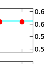
We first consider the convergence of the predictions in Eqs. (39) and (42) upon increasing the order of the truncation in Eq. (22). In Fig. 1 we report the estimates of , , and for , obtained with a non-vanishing background field, for various truncation orders . The values (red dots) display a rather small variation upon increasing , suggesting that their values have effectively converged to those corresponding to a full LPA solution. This fast convergence is due to the use of the optimized cutoff given by Eq. (58), as pointed out in Ref. Litim, 2002. While the values of and appear to be in very good agreement with the available MC data (shaded areas), the values of lie outside (though close to) the MC estimates.
In Tab. 1 we report the values of our best approximation for of and , comparing them with the MC and pRG estimates available in literature. For what concerns the values given by pRG, we report for the result of the three-loop Borel summation procedure Prudnikov et al. (2017), while for we report the low Padé approximation of the two-loop calculation Calabrese and Gambassi (2002).
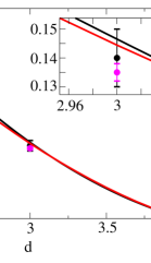
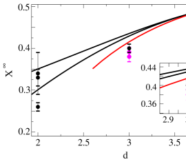
In Fig. 2, we report the predictions for and obtained with (red solid curve) as functions of the spatial dimensionality , and we compare them with MC (symbols) estimates and pRG predictions (black curves). The agreement between fRG and pRG predictions for is remarkable for , while increasing discrepancies emerge at smaller values of . The fRG predictions cannot be extended down to with the Ansatz considered. In fact, for additional stable fixed points appear beyond the Wilson-Fisher one, while for the latter disappears. This is not surprising, since for there exist more relevant terms than those considered in the truncation, which therefore is no longer sufficient and justified.
Concerning the values of , the predictions of fRG correspond to that of pRG close to , but it departs quite soon from it. The fRG prediction is much closer to the MC estimate in than the pRG one, although still not within its error bars.
The significant improvement provided by the fRG compared to the pRG can be traced back to two reasons. First, the LPA approximation provides a resummation of one-loop diagrams, resulting in a more precise determination of the amplitudes and , compared to the pRG predictions at order ; a comparison of the analytical expressions between pRG and fRG at order in LPA approximation is presented in Tab. 2. Second, the non-perturbative nature of the fRG provides a more accurate estimate of (see Fig. 2, left panel) and therefore of .
VI Conclusions and perspectives
In this work we presented an approach, based on the functional renormalization group (fRG), to predict the universal fluctuation-dissipation ratio (FDR) for the aging dynamics of model A. By calculating the two-time correlation functions from the renormalized effective action, we showed that, within the local potential approximation (LPA), the universal ratio depends only on the critical initial-slip exponent . As a side result, we proposed an alternative way to calculate within the fRG by focusing on the long-time behavior of the two-time response and correlation functions. Moreover, we showed that the values of and converge quickly upon increasing the order of the truncation in the Ansatz for the potential. Finally, we compared our prediction with the existing estimates obtained from Monte Carlo (MC) simulations and from the perturbative renormalization group (pRG), finding that the fRG results are closer to the MC than those of pRG ones.
Since the value of in is still not compatible with the MC results (although closer to it than predicted by previous approaches), a natural future direction is the computation of the two-time correlation functions beyond the LPA. Non-local terms are in fact expected to provide sizeable corrections, as they contribute with a term proportional to in the pRG Calabrese and Gambassi (2002). This could be achieved by using different approximations for closing the infinite hierarchy of equations generated by the fRG equation, following, for instance, the approach of Ref. Kloss et al., 2012 or considering mode-coupling approximations Bouchaud et al. (1996).
Other natural directions consist in applying our method to characterize the FDR of other static universality classes, e.g., and Potts models, or dynamics with conserved quantities Oerding (1993a, b). Moreover, the extension of the FDR analysis to non-equilibrium quantum systems Langen et al. (2016); Sieberer et al. (2013); Altman et al. (2015); Nicklas et al. (2015); Chiocchetta et al. (2017); Prüfer et al. (2018); Erne et al. (2018) represents an intriguing issue.
Acknowledgements.
We are indebted to R. Ben Alì Zinati and M. Scherer for useful discussions. A. C. acknowledges support by the funding from the European Research Council (ERC) under the Horizon 2020 research and innovation program, Grant Agreement No. 647434 (DOQS). M. V. warmly thanks the University of Milan and SISSA for their hospitality during the first phases of this project.Appendix A Effective action
Starting from the -dependent action , we define the associated generating function as
| (46) |
where denotes functional integration over both the fields and , while is an external field. Introducing the expectation value , where the average is taken with respect to the action , it is straightforward to check that the second derivative of with respect to is given by Berges et al. (2002)
| (47) |
where denotes the -dependent two-point function, whose entries are given by the and -dependent version of the response (4) and the correlation (5) functions. Finally, the -dependent effective action is defined as the modified Legendre transform of , given by
| (48) |
where is fixed by the condition
| (49) |
The definition of in Eq. (48) is such that Berges et al. (2002) , i.e., when is equal to the ultraviolet cutoff of the theory, the effective action reduces to the “microscopic” action evaluated on the expectation value . The following relationship can then be derived Berges et al. (2002):
| (50) |
Appendix B fRG flow equations
In this appendix we first present the detailed calculation of Eq. (28) with and . Then, the fRG flow equations for the corresponding couplings which appear in Eq. (22) are obtained explicitly for the case of vanishing background fields. Details concerning the non-vanishing background Ansatz are then discussed. Finally, we focus on the case , providing analytical formula for the time-dependent part of the fRG flow equations for the various couplings.
B.1 Calculation of and
Here we want to determine in Eq. (25), defined as in Eq. (50), but after replacing with its field-independent part. In order to do so, the matrix structure of the second variation of the modified effective action is set to
| (51) |
In order to implement the LPA truncation, above has to be computed on the basis of the expression for given in Eq. (21). Moreover, in order to separate the field-independent contribution from the field-dependent one , we proceed as explained in what follows. We first set
| (52) |
where the dispersion relation is given by
| (53) |
with
| (54) |
Accordingly, we define the field-dependent part (we assume for simplicity), as
| (55) |
The condition that in the definition of in Eq. (54) is chosen in order to expand the remaining field-dependent part as a power series of . This allows one to use a truncation procedure similar to that in the simple case of vanishing background field discussed at the end of Sec. III.1, as we discuss also below in App. B.4.
After a Fourier transform in space, is obtained from Eq. (52):
| (56) |
where
| (57a) | |||
| (57b) | |||
We note that in Eq. (56) the vanishing entry is due to the fact that the field-independent part of the second derivative of with respect to evaluated in the minimum configuration vanishes, as a consequence of causality Täuber (2014). Moreover, the correlation function in Eq. (57) respects the Dirichlet condition, which is enforced in our Ansatz, as described near Eq. (21).
B.2 Calculation of and
In order to calculate the ’s terms in Eq. (28) we use the so-called optimized regulator Litim (2000) , given by
| (58) |
First, note that fulfills the conditions in Eqs. (17), introduced in order to construct the fRG equation. By using the optimized cutoff function above it is possible to compute analytically the relevant integrals appearing in the ’s terms. This is due to two simplifications: first, the -derivative of the cutoff function in Eq. (28) is given by a theta function which vanishes for , i.e., . This implements a modified ultraviolet cutoff in the integrals in Eqs. (28). The second simplification, which is a consequence of the first, is due to the fact that the modified dispersion relation in Eq. (53) simplifies to in the interval allowed by . The regulator thus implements an infrared cutoff , rendering the dispersion indipendent of for . Accordingly, the two-time function in Eq. (56) becomes independent of the momentum , and will be simply indicated by .
The first term that we need to calculate is , given by Eq. (28) with . Taking advantage of these two simplifications, the dependence, contained in the -derivative of the cutoff function, can be factorized and the following expression for is obtained:
| (59a) | ||||
| (59b) | ||||
where is the entry of the matrix defined in Eq. (55), while the time-dependent function is defined as
| (60) |
with . The non-diagonal terms of do not appear in the final result (59), as required by causality Täuber (2014), since they would be multiplied by a factor . Then, by computing the trace in Eq. (60) one finds
| (61a) | ||||
| (61b) | ||||
| (61c) | ||||
where, in order to obtain Eq. (61b), we have used the expression of in Eq. (57b) together with the LPA property, which follows from Eq. (57a), that , and we have performed the integral over ; in order to obtain Eq. (61c), the time integral over has been computed by using the analytical expression of given in Eq. (57a). Finally, the expression of , where the Ansatz for is still unspecified, is given by Eq. (59), together with Eq. (61c).
The term is more complicated than the previous one since, unlike , it involves fields evaluated at different time coordinates. In fact, following the steps with which we have obtained Eq. (59), but for the case in Eq. (28), one obtains
| (62) |
where the two-time-dependent function is given by
| (63) |
In Eq. (62) we have retained only the contribution proportional to , i.e., proportional to (see Eq. (55)), since they are the only ones which renormalize the couplings , as one can see from their definition in Eq. (23). Other contributions, which renormalize the noise term , are discussed in Ref. Chiocchetta et al., 2016. As one can see from Eq. (62), the kernel is a two-time function from which one has to extract its local part, accordingly to the LPA Ansatz (21), in order to obtain the contribution of the ’s proportional to the terms which contain the coupling terms. This can be achieved by substituting in Eq. (62) Chiocchetta et al. (2016). Other contributions, which renormalize the derivative term , are discussed in Ref. Chiocchetta et al., 2016. If the previous substitution is made, Eq. (62) becomes
| (64) |
where the superscript denotes the local part of defined in Eq. (63), i.e.,
| (65a) | ||||
| (65b) | ||||
| (65c) | ||||
In order to obtain Eq. (65b) we have computed the trace in Eq. (63) and then the intermediate time integrals over and , similarly to what has been done in the computation of Eq. (60) leading to Eq. (61c). In order to obtain Eq. (65c), we computed the time integral over in Eq. (65b) by using the analytic expression of in Eq. (57a). Finally, the local part of , proportional to , is given by Eq. (64) together with in Eq. (65c). We have thus shown explicitly how the extraction of the local contribution in is implemented in the simple case of .
B.3 Case with and
Here we want to derive the fRG flow equation for the parameter and introduced in the Ansatz for the effective potential given by Eq. (29), for which , as discussed in Sec. III.2. The field-dependent part of is given by Eq. (30). Then, by taking advantage of Eq. (59), with Eqs. (64) and (30), one obtains
| (66) |
where we have considered only linear contributions in , in order to obtain the fRG flow equations of the coupling terms in Eq. (23), given by and . The time-dependent functions and are the same as those obtained previously, given by Eqs. (61c) and (65c) respectively, with the dispersion relation , with .
B.4 Case with and
The construction of the fRG equations for the couplings which define the Ansatz for the effective potential , given in Eq. (33), is discussed here for the case of non-vanishing background analyzed in Sec. III.3. According to the definition of in Eq. (55), one finds
| (67) |
where we define
| (68) |
while is defined according to Eq. (56) with as in Eq. (54) given by
| (69) |
ensuing from definition (54). The use of the invariants and introduced in Eq. (68) is customary in the context of fRG Delamotte (2012) and it helps in simplifying the notation in what follows. The form of in Eq. (67) allows us to express the r.h.s. of the fRG equation (27) as a power series of : this is done in the spirit of the discussion below Eq. (30). Accordingly, together with the vertex expansion (23), this provides a way to unambiguously identify the renormalization of the terms appearing in the potential in Eq. (33). In fact, and the coupling are identified as Delamotte (2012)
| (70) |
where the first condition actually defines as the minimum of the potential. In terms of the effective action , Eqs. (70) become
| (71) |
By taking a total derivative with respect to of each equality in Eqs. (71), one finds
| (72) | |||
| (73) |
which, after replacing with the fRG equation (19), render the flow equations for and . For the case of the potential in Eq. (33), by using Eq. (71), the set of flow equations (72) and (73) simplifies as
| (74) | ||||
| (75) |
where we used Eq. (27) with and defined in Eqs. (28) in terms of the in Eq. (67). The explicit form of the flow equations comes from a calculation analogous to the one discussed in Sec. III.2 and then detailed in App. B.2 (see Eqs. (59) and (64)). In particular, the flow of , defined in Eq. (69), takes contributions from the flow equations for both and .
Then, it is possible to construct the fRG flow equations for the dimensionless couplings
| (76) |
analogous to Eqs. (32). Considering the solutions of the fRG equations with vanishing -derivative of these dimensionless parameters one obtains equations similar to Eqs. (32) that finally allows the determination of the fixed point values. In order to solve these fRG equations, one has to supplement them with those involving the anomalous dimension (34), as one can see from the expression of the ’s terms computed in Eqs. (59) and (64).
B.5 Higher-order ’s terms
We discuss here what happens in the general case, i.e., with . Correspondingly, all the ’s terms with up to have to be computed. For these terms the associated time-dependent function , that appear in Eqs. (59) and (62) for and respectively, depend upon different times. The procedure for extracting the local contributions, with which we have obtained the last equation in Eq. (64), has to be extended to all the times other than . In order to retain linear contribution in , as before, it suffices to replace . In fact, one can show that the structure of Eqs. (61c) and (65c) is robust for higher-order terms () and all of them leads to terms of the form
| (77) |
with being a polynomial in . Accordingly, the exponential decay over time of the fRG flow equations (31) is a general feature within LPA approximation. Because of this, one can recover the long-time equilibrium fRG equations. This last equation is the proof of the statement done in the main text about the fact that any time-dependence in the fRG flow equation is of the exponentially decaying form as the one in Eqs. (31); accordingly, the equilibrium flow equations are retrieved in the long-time limit, since , as discussed around Eq. (34) in the main text.
In addition, by inspection of the time-dependent part of the ’s terms and based on previous considerations, an analytical formula for any localized kernel can be obtained as
| (78a) | ||||
| (78b) | ||||
where in the second equality is defined as
| (79a) | ||||
| (79b) | ||||
and we used the analytical expression of given by Eq. (57a). We note that Eq. (78a) reproduces Eqs. (61b) and (65b) respectively for and . Finally, Eq. (79b) is simply obtained by computing the integral over in Eq. (79a) with given in Eq. (57a).
The formulas in Eqs. (78b) and (79b) are very useful in order to implement analytically the LPA approach discussed here for the case of higher-order terms (), thus calculating the corresponding from the comparison with Eq. (77). Taking advantage of these analytical formulas a code in Mathematica has been used to compute the ’s terms for up to , as explained in Sec. V.
Appendix C Long-time aging regime
In this appendix, we first detail how in the absence of the background field the aging regime for the response and the correlation functions, given by Eqs. (41), is obtained. Then we consider the effect of the presence of a background field, detailing the way in which we obtain the expression for the reduced parameter , needed for solving Eqs. (44). Finally, we compare our results for with those obtained in Ref. Chiocchetta et al., 2016, proving the equivalence of these two approaches.
C.1 Case
Here we detail the calculations that led to the predictions of the response and the correlation functions in the aging regime, given by Eq. (41), for the case of vanishing background field with , starting from Eqs. (36) and given by Eq. (40). The response function in Eqs. (41) is readily obtained in the long-time limit of the aging limit, solving Eq. (36a) with given by Eq. (40) with . For the correlation function it is less straightforward to extract the behavior in the aging regime: one can rewrite Eq. (36b) as
| (80) |
where we used the identity , which follows from the LPA approximation (36a). Accordingly, the integral in the equation above should be computed in the regime . This amount of studying
| (81) |
where
| (82) |
The LPA prediction for the parameter in the case of a critical quench of the model is given by Eq. (38), that we report here
| (83) |
where is a function which decays exponentially fast as grows. Let us simplify the integral in Eq. (81), taking advantage of Eqs. (82) and (83):
| (84) |
where, in the last equality, we made the following changes of variable: and .
We recall that the aging regime is reached for . We break the integral in which appears in Eq. (84) as . The integral is given, in the aging limit, by , where we assumed that . In the following, we prove that the remaining integral over gives a vanishing contribution. To do so, we break the integral in which appear in Eq. (84), as . Since the integral over converges, it gives an overall vanishing contribution when integrated over in the aging regime. Let us now focus on the remaining integral given by
| (85) |
With the change of variable we obtain
| (86) |
and, as long as , this integral gives a vanishing contribution in the aging limit to the limit expression given by Eq. (81).
C.2 Case
Here we discuss how, in the presence of a background field, one can solve the equations (44) for the reduced two-time functions.
First, we prove that equations similar to Eqs. (38) and (40) can be obtained for the reduced parameter which enters Eq. (44). In order to obtain these equations one can use a simplification that appears at the level of the flow equation for it, i.e.,
| (88) |
In fact, according to our previous analysis, we retain only the explicit time dependence of which appears in the ’s terms, as we have discussed in Sec. III.1 near Eqs. (31). This amounts to the fact that the second term on the r.h.s. in the previous equation is time-independent, thus it will simply renormalize and therefore the value it has to take in order to obtain a vanishing long-time limit of , as we did in order to obtain Eq. (38) from Eq. (31a) in Sec. IV.2.
The fRG equation (88) for the reduced parameter is obtained, e.g., for the case of the non-vanishing background field Ansatz with , once the corresponding flow equation for and are derived, as explained in Sec. IV.3. Accordingly, the flow equation of is proportional to field derivatives of and , given by Eqs. (74) and (75). Thus, it is proportional to and , given explicitly by Eqs. (61c) and (65c). These two terms are equivalent for the analysis that follows, since their time dependence is always through .
Considering only one of these terms, the flow equation for the reduced parameter given by
| (89) |
where is given by the dimensionless time-independent part of the corresponding fRG flow equation ( in Eq. (31a)), and is an exponentially vanishing function of its argument. In the vicinity of the infrared fixed point, i.e., for , the factor behaves as , while , as a consequence of Eq. (34).
The critical initial-slip exponent is calculated from the integral over the cutoff of Eq. (89) (see the discussion which leads to Eq. (39) and apply it to the case of non-vanishing background Ansatz, i.e., replacing with its reduced version , as explained in Sec. IV.3). In the vicinity of the infrared fixed point, one finds
| (90a) | ||||
| (90b) | ||||
where means that the initial parameter is tuned in order to have for , as explained in the main text around Eq. (37), and the substitution is made in order to obtain Eq. (90b). This equation is the proof of the statement done in the main text about the fact that relations similar to Eqs. (38) and (40) are obtained also in the non-vanishing background field approximation for the reduced parameter .
C.3 Comparison with the short-time analysis
Here we compare the predictions derived in Sec. IV for with those obtained in Ref. Chiocchetta et al., 2016. There, was calculated via an analysis of the short-time behavior, i.e., focusing on the limit in which the waiting time is approximately the initial time , i.e., . From general scaling arguments for the aging dynamics Calabrese and Gambassi (2004) the anomalous dimension of the boundary field is related to by Chiocchetta et al. (2016)
| (91) |
In the case with and given by Eq. (29), , according to the fact that in the lowest order of LPA no anomalous dimension arises. Moreover, the anomalous dimension of the boundary field, given in Ref. Chiocchetta et al., 2016 by Eq. (46) with , matches the one which can be extracted from Eq. (39) by comparing it with Eq. (91). Accordingly, the analysis of the short-time behaviour done in Ref. Chiocchetta et al., 2016 and at long times presented here provide the same prediction for , as it should be, given that the scaling functions (9) are attained in the regime , which encompasses both cases. The equivalence between the two methods for calculating is also valid in the non-vanishing background field approximation, as described in what follows.
In the general case, it follows from the comparison of Eq. (91) with Eq. (90b) that
| (92) |
From the previous idenitification of (see below Eq. (89)) and computing the integral over from to of which appear in Eq. (92), where with , it follows that ; this expression is exactly Eq. (46) in Ref. Chiocchetta et al., 2016 and Eq. (39) obtained here with .
In order to prove the equivalence between the two methods we consider the analytical formula that, in Ref. Chiocchetta et al., 2016, has been used in order to calculate the anomalous dimension of the boundary fields , which is given by
| (93) |
where only the time dependent part in Eq. (89), i.e., is retained. Accordingly, Eq. (93) matches exactly with Eq. (92) if the substitution is made. The equivalence of the two approaches then follows.
Appendix D Expression of for and
Here we provide the correct expression of for the case of non-vanishing background field with , fixing a mistake in Ref. Chiocchetta et al., 2016 (see Eq. (45) and discussion around it). For completeness, we further provide the details which allow the numerical computation of . First, the equations for the fixed-point dimensionless couplings , and defined above Eq. (32) are given by (the superscript ∗ which henceforth we omit denotes fixed point values),
| (94a) | ||||
| (94b) | ||||
| (94c) | ||||
where and the dimensionless couplings and are defined in Eq. (76), while has been defined as
| (95) |
Note that in Ref. Chiocchetta et al., 2016 this definition of was used, although the text therein reported a definition without the factor at the denominator. Since Eqs. (94) depend upon the anomalous dimension , one has to supplement them with the equation for it, given by
| (96a) | ||||
| (96b) | ||||
where we have reported also the anomalous dimension related to the derivative parameter and the noise term . From Eqs. (94), using Eq. (96a), one can calculate numerically the fixed point values () depending on the spatial dimensionality , as we have done using Eqs. (32) in the main text. We find numerically (using Wolfram Mathematica 12.3.1) the following fixed point values of the rescaled couplings in (up to the second significant digit):
| (97) |
The values of the anomalous dimensions at this fixed point are found by replacing directly Eq. (97) into the expressions (96a) and (96b). The dynamical critical exponent is given by the second of Eqs. (34). In order to compute , we use the general scaling relation for , given by Eq. (91), and the value of obtained via a long-time analysis of the dynamics, one can focus on the anomalous dimension of the boundary field. Following the calculations discussed in Apps. C.2 and C.3 one obtains
| (98) |
We note that the analysis presented in Ref. Chiocchetta et al., 2016 led to a wrong expression for , given by Eq. (G6) (not reported here). In fact, as discussed here in the main text, they missed to add to the term proportional to (see Eq. (45) for the correct equation for ). The computation of follows via Eq. (91), once the dimensionless fixed-point values of , and are calculated. For instance, using the values Eq. (97), one obtains for . Finally the universal amplitude ratio is calculated accordingly to Eq. (42).
References
- Privman et al. (1991) V. Privman, P. Hohenberg, and A. Aharony, in Phase Transitions and Critical Phenomena, Vol. 14, edited by C. Domb and J. L. Lebowitz (Academic Press New York, 1991).
- Henkel et al. (2008) M. Henkel, H. Hinrichsen, and S. Lübeck, Non-Equilibrium Phase Transitions: Volume 1 (Springer, 2008).
- Henkel et al. (2011) M. Henkel, H. Hinrichsen, M. Pleimling, and S. Lübeck, Non-Equilibrium Phase Transitions: Volume 2 (Springer, 2011).
- Schmittmann and Zia (1995) B. Schmittmann and R. Zia, Statistical Mechanics of Driven Diffusive Systems, edited by C. Domb and J. Lebowitz, Phase Transitions and Critical Phenomena, Vol. 17 (Academic Press, 1995).
- Bouchaud et al. (1997) J.-P. Bouchaud, L. F. Cugliandolo, J. Kurchan, and M. Mézard, “Out of equilibrium dynamics in spin-glasses and other glassy systems,” in Spin Glasses and Random Fields (1997) pp. 161–223.
- Hinrichsen (2000) H. Hinrichsen, Adv. Phys. 49, 815 (2000).
- Täuber (2014) U. C. Täuber, Critical Dynamics (Cambridge University Press, 2014).
- Mitra et al. (2006) A. Mitra, S. Takei, Y. B. Kim, and A. J. Millis, Phys. Rev. Lett. 97, 236808 (2006).
- Scheppach et al. (2010) C. Scheppach, J. Berges, and T. Gasenzer, Phys. Rev. A 81, 033611 (2010).
- Schole et al. (2012) J. Schole, B. Nowak, and T. Gasenzer, Phys. Rev. A 86, 013624 (2012).
- Langen et al. (2016) T. Langen, T. Gasenzer, and J. Schmiedmayer, J. Stat. Mech.: Theory Exp. 2016, 064009 (2016).
- Sieberer et al. (2013) L. M. Sieberer, S. D. Huber, E. Altman, and S. Diehl, Phys. Rev. Lett. 110, 195301 (2013).
- Altman et al. (2015) E. Altman, L. M. Sieberer, L. Chen, S. Diehl, and J. Toner, Phys. Rev. X 5, 011017 (2015).
- Nicklas et al. (2015) E. Nicklas, M. Karl, M. Höfer, A. Johnson, W. Muessel, H. Strobel, J. Tomkovič, T. Gasenzer, and M. K. Oberthaler, Phys. Rev. Lett. 115, 245301 (2015).
- Chiocchetta et al. (2015) A. Chiocchetta, M. Tavora, A. Gambassi, and A. Mitra, Phys. Rev. B 91, 220302 (2015).
- Chiocchetta et al. (2017) A. Chiocchetta, A. Gambassi, S. Diehl, and J. Marino, Phys. Rev. Lett. 118, 135701 (2017).
- Prüfer et al. (2018) M. Prüfer, P. Kunkel, H. Strobel, S. Lannig, D. Linnemann, C.-M. Schmied, J. Berges, T. Gasenzer, and M. K. Oberthaler, Nature 563, 217 (2018).
- Erne et al. (2018) S. Erne, R. Bücker, T. Gasenzer, J. Berges, and J. Schmiedmayer, Nature 563, 225 (2018).
- Young et al. (2020) J. T. Young, A. V. Gorshkov, M. Foss-Feig, and M. F. Maghrebi, Phys. Rev. X 10, 011039 (2020).
- Diessel et al. (2021) O. K. Diessel, S. Diehl, and A. Chiocchetta, (2021), arXiv:2103.01947 [cond-mat.quant-gas] .
- Bouchaud et al. (2009) J.-P. Bouchaud, J. D. Farmer, and F. Lillo, in Handbook of Financial Markets: Dynamics and Evolution, Handbooks in Finance, edited by T. Hens and K. R. Schenk-Hoppé (North-Holland, San Diego, 2009).
- Szabó and Czárán (2001) G. Szabó and T. Czárán, Phys. Rev. E 63, 061904 (2001).
- Mobilia et al. (2007) M. Mobilia, I. T. Georgiev, and U. C. Täuber, J. Stat. Phys. 128, 447 (2007).
- Fruchart et al. (2021) M. Fruchart, R. Hanai, P. B. Littlewood, and V. Vitelli, Nature 592, 363 (2021).
- Janssen et al. (1989) H.-K. Janssen, B. Schaub, and B. Schmittmann, Z. Phys. B 73, 539 (1989).
- Janssen (1992) H.-K. Janssen, in From Phase Transitions to Chaos, Topics in Modern Statistical Physics, edited by G. Györgyi, I. Kondor, L. Sasvári, and T. Tél (World Scientific, Singapore, 1992).
- Calabrese and Gambassi (2005) P. Calabrese and A. Gambassi, J. Phys. A: Math. Gen. 38, R133 (2005).
- Hohenberg and Halperin (1977) P. C. Hohenberg and B. I. Halperin, Rev. Mod. Phys. 49, 435 (1977).
- Calabrese et al. (2006) P. Calabrese, A. Gambassi, and F. Krzakala, J. Stat. Mech: Th. Exp. 2006, P06016 (2006).
- Calabrese and Gambassi (2007) P. Calabrese and A. Gambassi, J. Stat. Mech: Th. Exp. 2007, P01001 (2007).
- Calabrese and Gambassi (2002) P. Calabrese and A. Gambassi, Phys. Rev. E 66, 066101 (2002).
- Chiocchetta et al. (2016) A. Chiocchetta, A. Gambassi, S. Diehl, and J. Marino, Phys. Rev. B 94, 174301 (2016).
- Dupuis et al. (2021) N. Dupuis, L. Canet, A. Eichhorn, W. Metzner, J. Pawlowski, M. Tissier, and N. Wschebor, Physics Reports 910, 1 (2021), the nonperturbative functional renormalization group and its applications.
- Kloss et al. (2012) T. Kloss, L. Canet, and N. Wschebor, Phys. Rev. E 86, 051124 (2012).
- Calabrese and Gambassi (2004) P. Calabrese and A. Gambassi, J. Stat. Mech.: Theory Exp. 2004, P07013 (2004).
- Cugliandolo et al. (1994) L. F. Cugliandolo, J. Kurchan, and G. Parisi, Journal de Physique I 4, 1641 (1994).
- Godrèche and Luck (2000) C. Godrèche and J. M. Luck, J. Phys. A: Math. Gen. 33, 9141 (2000).
- Berges et al. (2002) J. Berges, N. Tetradis, and C. Wetterich, Phys. Rep. 363, 223 (2002).
- Delamotte (2012) B. Delamotte, Lect. Notes Phys. 852, 49 (2012).
- Canet and Chaté (2007) L. Canet and H. Chaté, J. Phys. A: Math. Theor. 40, 1937 (2007).
- Grassberger (1995) P. Grassberger, Physica A 214, 547 (1995).
- Jaster et al. (1999) A. Jaster, J. Mainville, L. Schülke, and B. Zheng, J. Phys. A: Math. Gen. 32, 1395 (1999).
- Prudnikov et al. (2017) V. V. Prudnikov, P. V. Prudnikov, and M. V. Mamonova, Phys.-Uspekhi 60, 762 (2017).
- Prudnikov et al. (2008) V. V. Prudnikov, P. V. Prudnikov, I. A. Kalashnikov, and S. S. Tsirkin, J. Exp. Theor. Phys. 106, 1095 (2008).
- Litim (2002) D. F. Litim, Acta Phys. Slov. 52 (2002).
- Bouchaud et al. (1996) J.-P. Bouchaud, L. Cugliandolo, J. Kurchan, and M. Mézard, Physica A 226, 243 (1996).
- Oerding (1993a) H.-K. Oerding, K. Janssen, J. Phys. A: Math. Gen. 26, 5295 (1993a).
- Oerding (1993b) H.-K. Oerding, K. Janssen, J. Phys. A: Math. Gen. 26, 3369 (1993b).
- Litim (2000) D.-F. Litim, Phys. Lett. B 486, 92 (2000).