Near-Infrared Polarization from Unresolved Disks Around
Brown Dwarfs and Young Stellar Objects

Abstract

Wide-field near-infrared (NIR) polarimetry was used to examine disk systems around two brown dwarfs (BD) and two young stellar objects (YSO) embedded in the Heiles Cloud 2 (HCl2) dark molecular cloud in Taurus as well as numerous stars located behind HCl2. Inclined disks exhibit intrinsic NIR polarization due to scattering of photospheric light which is detectable even for unresolved systems. After removing polarization contributions from magnetically aligned dust in HCl2 determined from the background star information, significant intrinsic polarization was detected from the disk systems of of one BD (ITG 17) and both YSOs (ITG 15, ITG 25), but not from the other BD (2M0444). The ITG 17 BD shows good agreement of the disk orientation inferred from the NIR and from published ALMA dust continuum imaging. ITG 17 was also found to reside in a 5,200 au wide binary (or hierarchical quad star system) with the ITG 15 YSO disk system. The inferred disk orientations from the NIR for ITG 15 and ITG 17 are parallel to each other and perpendicular to the local magnetic field direction. The multiplicity of the system and the large BD disk nature could have resulted from formation in an environment characterized by misalignment of the magnetic field and the protostellar disks.

1 Introduction

Disks around low-mass objects offer unique insights into star and planet formation processes (see reviews by Luhman, 2012; Andrews, 2020), especially regarding low-mass star and brown dwarf formation. However, such objects are intrinsically faint and their disks less massive, posing challenges for studies of the dust emission from those disks using radio interferometers.

In addition to emitting thermal radiation, dust in disks also scatters and polarizes central object (and disk) light. Linear polarimetry observations and modeling of resolved disks (e.g., Silber et al., 2000; Apai et al., 2004; Follette et al., 2013; Esposito et al., 2018, 2020) have been used to constrain disk properties and to identify departures in the polarization patterns, and the structures seen in polarized light, as bona fide disk features (Avenhaus et al., 2014; Benisty et al., 2015; Asensio-Torres et al., 2016; Garufi et al., 2018), perhaps due to planet or protoplanet formation.

Near-infrared (NIR) polarimetry may offer an efficient way to survey, detect, and identify low-mass star or BD disks for follow-up examination by millimeter (mm) and submillimeter (submm) wavelength interferometers. This current study sought to use NIR polarimetry to probe two brown dwarf (BD) disks and two young stellar object (YSO) disks in Taurus to assess the efficacy of this method and to compare NIR and mm disk orientation findings.

Stars (or BDs) without disks are sources of unpolarized light. Polarization signals detected in the light from distant examples of such objects may be evaluated, for example, to trace magnetic field orientations in intervening dusty material along the line of sight (Hiltner, 1949a, b; Hall, 1949; Davis & Greenstein, 1951). However, those lines of sight may be long and feature complex dust and gas distributions, which complicates localizing magnetic field properties to particular atomic or molecular clouds of interest. Foreground and background polarization contributions from dust in the diffuse and dense interstellar medium (ISM) components can become mixed with any target object polarization, masking the desired signal. In this study, these polarization contributions were quantified and removed in order to isolate the intrinsic NIR polarization due to BD and YSO disks. This required determining the polarization properties of these foregrounds and backgrounds as well as developing accurate knowledge of the distances to the target disks along the line of sight so that removal of these extrinsic polarizing effects could be performed.

The Taurus star-forming region is one of the best studied laboratories for low-mass star formation (e.g., Elias, 1978; Beckwith et al., 1990; Kenyon et al., 1990) and sprawls across about $12\times 16^{\circ}$ of the sky (see the Figure 18-5-6 extinction map of Dobashi et al., 2005). Yet it has been only recently, with the release of Gaia DR2 (Gaia Collaboration et al., 2016, 2018) and the studies by Luhman (2018) and Galli et al. (2019), that accurate distances to the constituent dark clouds in Taurus and their associated groupings of stars, YSOs, and BDs have been established. These distances range from about 129 pc for B215 to 198 pc for L1558 (both from Galli et al., 2019). Hence, depending on the location of the Taurus objects under study, the foregrounds and backgrounds that will contribute unrelated polarization signals can vary considerably across the Taurus region.

Young, low-mass objects in different sub-regions of Taurus have been cataloged and investigated in previous studies. These include the Itoh et al. (1996, hereafter ITG) $1\times 1$° NIR survey of the Heiles Cloud 2 (hereafter HCl2) dark molecular cloud that found 831 sources, 50 of which were classified as young (YSO Class I or II). Their deep, higher resolution NIR survey (Itoh et al., 1999) of 23 of the young objects revealed five of the ITG objects also had faint, nearby ($<$ 6 arcsec) low-luminosity companions.

Multi-wavelength spectral energy distributions (SEDs) for many of the ITG objects and other young, low-mass stars and BDs in Taurus were developed and modeled by Andrews et al. (2013) to assess which had disks and envelopes and to ascertain many of the disk properties. Their SED fitting also refined the natures of the hosts and whether the systems suffered dust extinction and reddening arising outside of the host-disk system.

Portions of the Taurus system of dark clouds also have been probed to reveal magnetic field properties using background starlight polarimetry in the NIR using the Mimir instrument (Clemens et al., 2007) by Chapman et al. (2011) as well as through previously published optical and NIR studies (as reviewed in Chapman et al., 2011). Across much of Taurus, the predominant magnetic field orientation is perpendicular to the Galactic equator, a somewhat unusual condition not shared by most of the molecular material in the Galactic disk (Clemens et al., 2020).

In the current study, NIR polarimetry was performed using Mimir toward two sky fields in Taurus known to contain BDs with disks. Analysis of the NIR data, in combination with Gaia Early Data Release 3 (EDR3: Gaia Collaboration et al., 2016, 2020) proper motions and parallaxes as well as archival NIR and mid-infrared photometry were used to ascertain foreground, embedded, and background polarization and extinction properties. These were used to deduce the intrinsic NIR polarization properties of the disks around the two BDs and two YSOs.

The remainder of this paper is organized as follows. The target fields and objects, the Mimir observations, data processing steps, and apparent polarization properties of the objects in each field are described in Section 2. Identification of foreground, embedded, and background objects and the determination of the polarization signals contributed by the foreground and background ISM are described in Section 3. After correcting for the polarization contributions from HCl2, the resulting intrinsic polarization properties for the BDs and YSOs are presented in Section 3.6. Section 4 considers the origin of the NIR intrinsic polarization are argues that one BD-YSO pair constitutes a 5,200 au wide-binary with co-aligned disks. The past role possibly played by the magnetic field in HCl2 is assessed in light of the relative orientations of these disks and the local magnetic field orientation. Finally, Section 5 provides a project summary.

2 Target Fields and Observations

2.1 Brown Dwarf and Young Stellar Object Disk Targets

Analysis and modeling of archival ALMA continuum imaging, combined with other archival multi-band photometry, enabled Rilinger et al. (2019) to improve on the Andrews et al. (2013) models for the disks around two late-M type BDs in Taurus: ITG 17 (EPIC 248029954; CFHT Tau 4) and IRAS S04414+2506 (EPIC 247915927; 2M0444). The Rilinger et al. (2019) ALMA data analyses also partially resolved the two disks, yielding constraints on their major axis orientations and inclination angles, as well as other properties such as mass and inner and outer radii, which they sought to use to test BD formation models.

These two BD disk systems were selected for study using NIR polarimetry observations with the $10\times 10$ arcmin field of view Mimir instrument at the 1.8m Perkins Telescope Observatory (PTO). The two non-overlapping fields centered on these BD targets were designated the “CFHT Tau 4” and “2M0444” fields, following the target names used by Rilinger et al. (2019). Because the Mimir imaging polarimetry solid angle is large, field objects (both foreground and background) for both observed Mimir regions were simultaneously sampled for use in ascertaining the polarization signals contributed by the magnetic field of the intervening diffuse ISM and the denser HCl2 in Taurus.

The CFHT Tau 4 field contains an additional five ITG objects (ITG 15, 16, 19, 21, and 25). Two of these are YSOs with disks (ITG 15 and 25) that were in the Andrews et al. (2013) SED analysis study. They were added to the two BDs to become the four objects of this study. Three of the ITG objects (15, 21, and 25) were in the close companion survey of Itoh et al. (1999). As summarized in Appendix A, ITG 16, 19, and 21 were found to not be YSOs and not associated with HCl2 but instead to be unrelated background stars. Select properties for all of the ITG objects in this field, and those of their companions, are listed in Table 1 as are the properties of the BD in the 2M0444 field. Four (ITG 15, 17, 21, and 25) are doubles, identified using ‘A’ designations for the brighter primaries and ‘B’ for the fainter companions.

The 0.1 pc diameter dense core IRAS 04368+2557 (L1527) (Benson & Myers, 1989) and its embedded YSO Class 0/I source L1527 IRS (e.g., Chen et al., 1995; Motte & André, 2001; Tobin et al., 2008; Kristensen et al., 2012) are also located within the CFHT Tau 4 field observed by Mimir. The relation of the HCl2 magnetic field orientation to this dense core, YSO, and its disk and envelope will be considered in a future paper.

2.2 Near-Infrared Polarization Observations

Observations of the CFHT Tau 4 and 2M0444 fields were obtained with the Mimir instrument in its imaging polarimetry mode, which had a pixel field of view of $0.6\times 0.6$ arcsec onto a $1024\times 1024$ pixel ALADDIN III InSb detector array, at the PTO, located on Anderson Mesa, outside Flagstaff, AZ on the UT nights of 2019 December 13 and 21 as well as 2020 January 6, February 12 and 14. One polarimetric observation in the NIR $H$-band (1.6 $\mu$m) consisted of 96 images, obtained as single images for each of 16 distinct orientations of the cold half-wave plate within Mimir, for each of 6 sky dither positions, offset by 15–21 arcsec. Image integration times of 2.3, 10, and 15 sec were used for different observations. After evaluating the images in the multiple observations for sufficiently high quality, the total useful integration time for the CFHT Tau 4 and 2M0444 fields was 55 min each.

Dome flats, dark current, and sky observations of polarization standard stars all followed usual Mimir procedures, as described in Clemens et al. (2012a, b). Data processing also followed standard Mimir steps, resulting in a catalog of polarization values (a POLCAT, Clemens et al., 2012c) for each observation. The cataloged values for each object included the linear Stokes parameters $U$ and $Q$ (as percentages of Stokes $I$), the debiased polarization percentage $P^{\prime}$ , the equatorial polarization position angle (EPA, measured East from North), and the uncertainties in all these quantities.

Polarization quantities for objects contained in the six POLCATs for the CFHT Tau 4 field were combined for each matching object using Stokes $U$ and $Q$ averaging, weighted by their variances, followed by recovery of the raw polarization percentage $P$ (= $(U^{2}+Q^{2})^{0.5}$) and its uncertainty $\sigma_{P}$ for 121 objects in this field. The average seeing was about 2.1 arcsec. The same Stokes averaging was also performed for the five POLCATs obtained for the 2M0444 field, resulting in polarization information for 275 objects. The average seeing for this field was about 1.6 arcsec.

For objects with $P$ exceeding $\sigma_{P}$, the debiased $P^{\prime}$ was computed as $(P^{2}-\sigma_{P}^{2})^{0.5}$. For objects not meeting this criterion, $P^{\prime}$ was set to zero. Equatorial polarization position angles (EPA) were computed from the Stokes parameters, and their uncertainties were computed from the debiased polarization signal-to-noise ratio (SNR). Where $P^{\prime}$ was zero, EPA was also set to 0° and its uncertainty set to 180°.

Table 2 presents a shortened version of the electronic table that contains the NIR polarization values measured for the objects in the two fields. The first column offers R.A.-ordered field and object number designations. The next two columns provide J2000 R.A. and decl. values, both in degrees. The Mimir-based $H$-band magnitude is next, though users are cautioned that no color corrections have been applied (see Clemens et al., 2012b). The debiased polarization percentage $P^{\prime}$ and its uncertainty $\sigma_{P}$ are followed by the EPA and its uncertainty. The final four columns provide the Stokes $Q$ and $U$ values and their uncertainties.

=25mm

Table 1: Observed Fields and Selected Target Systems

Desig.	R.A.	decl.	Type	Sp. Typ.	Mass	Lumin.	Offset: from	Other Desig.
	(∘)	(∘)			($M_{\odot}$)	($L_{\odot}$)
(1)	(2)	(3)	(4)	(5)	(6)	(7)	(8)	(9)
CFHT Tau 4 Field     Centered at (R.A., decl. [J2000]) = (69.95°,+26.02°) - (L, B) = (173.84°,$-$13.56°)
ITG 15B	69.93648	+26.03192	…	…	0.009a	…	3.0-3.1′′: ITG 15Aa,b
ITG 15A	69.93700	+26.03131	YSO	M5c	0.17a	0.51d	…	IRAS F04366+2555,
					0.117b	0.088b		2MASS J04394488+2601527
ITG 16	69.94289	+25.95412	…i	…	…	…	…	2MASS J04394629+2557149
ITG 17A	69.94784	+26.02797	BD	M7c	0.095d	0.175d	37′′: ITG 15A	CFHT Tau 4,
								2MASS J04394748+2601407
ITG 17B	69.94899	+26.02744	…	…	…	…	4.2′′: ITG 17Aa
ITG 19	69.98784	+26.09035	…i	…	…	…	…	2MASS J04395708+2605252
ITG 21B	70.00722	+25.94132	…i	M5.5c,e	…	…	0.56′′: ITG 21Ae	(2MASS J04400174+2556292)e
ITG 21A	70.00736	+25.94141	…i	M5.5c,e	…	…	…	(2MASS J04400174+2556292)e
ITG 25B	70.03213	+26.08989	…	…	0.018a	…	4.3′′: ITG 25Aa
ITG 25A	70.03335	+26.09040	YSO	(K6–M3.5)d	0.19a	0.90d	…	IRAS 04370+2559,
				M2cf				2MASS J04400800+2605253
2M0444 Field     Centered at (R.A., decl. [J2000]) = (71.11°,+25.21°) - (L, B) = (175.16°,$-$13.27°)
2M0444	71.11309	+25.20456	BD	M7.25c	0.05g	0.028h	…	IRAS S04414+2506,
								2MASS J04442713+2512164

Note. — ^a from Itoh et al. (1999), ^b from Ward-Duong et al. (2018), ^c from Luhman et al. (2010), ^d from Andrews et al. (2013), ^e resolved by UKIDSS and Gaia DR2 and EDR3 but not by 2MASS or Mimir, ^f from Joncour et al. (2017), ^g from Ricci et al. (2013), ^h from Ricci et al. (2014), ⁱ see Appendix A

=25mm

Table 2: Observed Near-Infrared $H$-band Polarization Properties of Objects in the Fields

Desig.	R.A.	decl.	$m_{H}$	$P^{\prime}$	$\sigma_{P}$	EPA	$\sigma_{EPA}$	Stokes $Q$	$\sigma_{Q}$	Stokes $U$	$\sigma_{U}$
(Field-Num.)	(∘)	(∘)	(mag)	(%)	(%)	(°)	(°)	(%)	(%)	(%)	(%)
(1)	(2)	(3)	(4)	(5)	(6)	(7)	(8)	(9)	(10)	(11)	(12)
10001	69.846268	26.064350	13.822	2.256	1.317	71.3	16.7	$-$2.077	1.305	1.584	1.337
10002	69.848568	26.078516	14.349	1.191	1.851	53.7	44.5	$-$0.660	1.871	2.100	1.849
10003	69.849897	26.045857	16.650	0.000	18.765	0.0	180.0	$-$15.536	18.767	$-$0.982	18.383
…
20001	71.022033	25.209503	13.241	0.000	5.135	0.0	180.0	3.728	5.154	1.680	5.040
20002	71.024325	25.235553	13.403	1.501	0.773	17.4	14.8	1.385	0.771	0.965	0.777
20003	71.024721	25.233388	16.361	0.000	14.228	0.0	180.0	9.881	14.130	7.198	14.412

Note. — Table 2 is published in its entirety in the machine-readable format. A portion is shown here for guidance regarding its form and content.

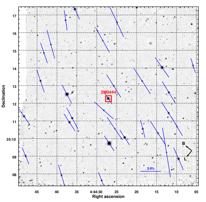
Figure 1: Mimir $H$-band image of the $10\times 10$ arcmin² field of view containing the BD 2M0444. Blue pseudo-vectors, with 2% reference pseudo-vector at lower right, show the $P^{\prime}$ lengths and EPA orientations for the 30 objects meeting the polarization detection criteria described in the text. The average EPA is about 27° and the Galactic plane is parallel to EPA 141°, as shown via the black B and L labeled vectors at lower right. Several galaxies appear in the image, consistent with the average A_V of 2-3 mag for the field. (Figure 11 shows a zoomed view of the central region.)

2.3 Apparent Polarization Maps

Figure 1 displays the combined Mimir $H$-band image for the 2M0444 field. The 30 stars that met polarization quality criteria of $\sigma_{P}\leq 1.5$%, polarization signal-to-noise $PSNR\equiv(P/\sigma_{P})\geq 2$, and $m_{H}\leq 16.4$ mag are shown as blue pseudo-vector lines (lacking ends). The lengths of the lines are proportional to the $P^{\prime}$ values and their orientations show the EPA values. The central BD 2M0444 (object 20153 in Table 2) was significantly detected, exhibiting $P^{\prime}$  $=1.29\%\pm 0.24$% and EPA $=34\arcdeg\pm 5$° in the $H$-band. The unweighted average EPA of the polarization-detected objects is $26\arcdeg.6\pm 1.\arcdeg 7$, while the disk of the Milky Way has an EPA of about 141°. The similar average of $P^{\prime}$ values is $2.33\%\pm 0.12$%. For the 27 polarization-detected objects that have 2MASS (Skrutskie et al., 2006) matches, the average $(H-K)$ color is $0.273\pm 0.011$ mag. Following the Near-Infrared Color Excess (NICE) method (Lada et al., 1994), the average extinction A_V is 2.3 mag for those objects.

Figure 2 shows the Mimir image for the CFHT Tau 4 field, with the 20 polarization-detected objects drawn as blue lines. One low-polarization object, described in Appendix C, is shown by a green circle. All six ITG objects, labeled with red boxes, had NIR values that met the three polarization selection criteria. The average $P^{\prime}$ for the 20 polarization-detected objects is $2.81\%\pm 0.27$% at an average EPA of $54\arcdeg\pm 4$°. However, the $P^{\prime}$ values for the YSO ITG 15 (object 10073 in Table 2) and the BD ITG 17 (object 10080; CFHT Tau 4) are far below the average, at $0.44\%\pm 0.08$% and $0.26\%\pm 0.11$%, respectively. The YSO ITG 25 (object 10117) shows a greater than average $P^{\prime}$ of $4.08\%\pm 0.10$%. For the 20 object sample, the mean $(H-K)$ color is $0.65\pm 0.06$ mag, implying an average A_V of 8.2 mag for this field. More objects are visible in the bottom and right portions of the Figure, while an absence of objects is noted in the upper left where one outflow lobe of L1527 IRS (Cook et al., 2019) is seen as the extended faint feature East of IRS.

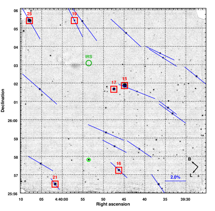
Figure 2: Mimir $H$-band image of the CFHT Tau 4 field containing the BD ITG 17 (aka CFHT Tau 4) and the two YSOs ITG 15 and 25. Red squares identify the six objects with ITG (Itoh et al., 1996) numbers. Blue pseudo-vectors, with 2% reference pseudo-vector at lower right, show the $P^{\prime}$ lengths and EPA orientations for the 20 objects meeting the polarization detection criteria described in the text. One object bright enough to show polarization, but failing the $PSNR$ criterion is indicated by a light green circle at lower left (see Appendix C). The location of the L1527 IRS source is indicated by a dark green circle and label at upper left. The mean polarization EPA is 54^∘, which is perpendicular to the Galactic equator orientation of 140°. However, both ITG 15 and ITG 17 exhibit distinctly different polarization values than seen in the remainder of the field. (Figure 10 shows a zoomed version about these two objects.)

3 Analyses

Analyses began with establishing distances to the BDs and stars that had been measured for polarization, using Gaia Early Data Release 3 (EDR3; Gaia Collaboration et al., 2020) parallaxes and proper motions, as described in Section 3.1. The properties of the extincting molecular cloud material were established via stellar reddening and molecular gas emission map comparisons, in Section 3.2. Locations were determined for the BD objects and YSOs from their extinctions, relative to the local HCl2 values, and the effects of foreground polarization on the BD and YSO disk polarization signals were quantified. The ITG 17 and 2M0444 BDs, as well as the YSOs ITG 15 and ITG 25, were found to reside within HCl2, as described in Section 3.3.

In Section 3.4, characterization and removal of the polarization signals added by the passage of the light from the BDs and YSOs through magnetically aligned dust in HCl2 revealed the intrinsic BD and YSO disk polarization properties (Section 3.6). These were compared to the properties found for the dust thermal emission from the disks detected using ALMA by Ricci et al. (2014) and Rilinger et al. (2019).

3.1 Cloud and Object Distances

Vizier (Ochsenbein et al., 2000) was used to fetch Gaia EDR3, 2MASS (Skrutskie et al., 2006), UKIDSS (Lawrence et al., 2007) Galactic Cluster Survey (Lodieu et al., 2009), and WISE (Wright et al., 2010) entries across the solid angles spanned by the two Mimir fields. These stellar entries were position-matched to the Mimir $H$-band POLCAT entries for each field, using topcat (Taylor, 2005), resulting in tables containing the polarimetry, multi-band photometry, parallax, and proper motion data for the objects.

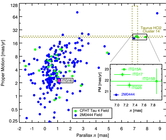
Figure 3: Plot of Gaia EDR3 proper motion amplitude versus parallax for objects in the two sky fields. The vertical axis displays the proper motion amplitude, scaled as the base-2 log to show the full range of values. The means and standard deviations of the values for cluster 14 of Galli et al. (2019) in Taurus HCl2 are indicated by the vertical and horizontal olive-green dashed rectangles. Four of the CFHT Tau 4 field ITG objects and 2M0444 have Gaia EDR3 matches and are labeled with the same color as their field. No objects in the CFHT Tau 4 field (filled green circles) are located closer than the indicated ITG objects. One object in the 2M0444 field (filled blue circles) is closer than the BD in that field. ITG 16 in the CFHT Tau 4 field, labeled next to its magenta filled circle, has Gaia EDR3 parallax and proper motion values placing it far more distant than HCl2. Inset: Expanded view of proper motion and parallax for the objects inside the boxed region shown near the cluster 14 label. Error bars shown indicate Gaia EDR3 $\pm$1 $\sigma$ uncertainties.

Luhman (2018) and Galli et al. (2019) analyzed the Gaia DR2 parallaxes and proper motions over much larger portions of the Taurus cloud complex, establishing accurate distances to the individual molecular clouds making up the Taurus complex and finding groups of objects exhibiting similar distances and proper motions. Galli et al. (2019) used cluster analysis techniques to identify more distinct star groups than Luhman (2018) by also including spatial clustering. Of the 21 clusters Galli et al. (2019) identified and characterized (but noting that these could be unbound groupings of objects that merely exhibit similar distances, motions, and spatial locations), their cluster 14 best matches the BD and YSOs in the CFHT Tau 4 field and the 2M0444 BD. Indeed, ITG 15A and 17A as well as 2M0444 are contained in the cluster 14 inventory reported in Appendix A of Galli et al. (2019), while the remaining YSO, ITG 25A, they assigned to their cluster 15.

Figure 3 shows the amplitude of proper motion versus parallax for objects in the two Mimir fields that had such information listed in Gaia EDR3. The means and standard deviations of the amplitude of proper motion and the parallax for cluster 14 from Galli et al. (2019) are shown as the vertical and horizontal olive-green dashed rectangles that pass through the groupings of ITG objects plus 2M0444. The Gaia measured uncertainties in proper motions and parallaxes depend strongly on brightness, ranging from 0.045 to 1.76 mas yr^-1 for 2M0444 and ITG15B, respectively, and 0.057 to 1.20 mas for ITG 15A and ITG 15B, respectively. One finding from Figure 3 is that to the limits of Gaia EDR3, no significant foreground stellar population was revealed. The improved Gaia EDR3 values, displayed in the Figure 3 inset, tighten the proper motion and parallax ranges with respect to the Gaia DR2 values, confirming that the four ITG objects are part of the same association in Taurus at a distance of 139.6$\pm$1.0 pc, computed as the inverse of the weighted parallax mean and propagated uncertainty. The distance to 2M0444 is similar, though greater by 3.6$\pm$1.6 pc.

3.2 Cloud Structures and Extinctions

Extinction maps by Dobashi et al. (2005) and Lombardi et al. (2010) have revealed the distribution of dust in Taurus, while the molecular gas has been traced by Narayanan et al. (2008) using CO and ¹³CO. Here, the molecular gas distribution in each field was obtained from the Narayanan et al. (2008) data as a line-integrated ¹³CO spectral line map by limiting the radial velocity integration window to be from 0 to 12 km s^-1. This gas tracer is expected to faithfully reveal gas column densities, provided the gas is not too diffuse, so that molecular self-shielding fails and dissociation dominates, and provided the the gas is not too volumetrically dense, so that CO is depleted as mantles onto dust grains (c.f., Pineda et al., 2010). In HCl2, both of these processes likely occur, so the molecular maps will be only partially representative of the gas properties along these lines of sight.

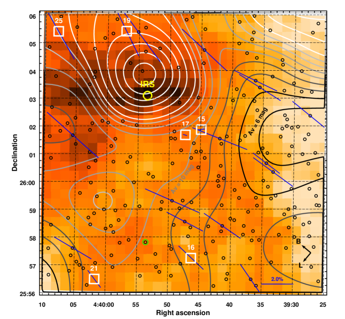
Figure 4: Map of ¹³CO line-integrated emission and extinction A_V across the CFHT Tau 4 field. The color image shows ¹³CO integrated emission, from Narayanan et al. (2008), ranging from about 2.3 K km s^-1 for the lightest yellow colors up to about 5.1 K km s^-1 for the darkest colors, at about 45 arcsec resolution. The contours indicate inferred A_V values, at about 2 arcmin resolution, derived from the $(H-M)$ colors of the objects but not including the ITG objects. Contours trace 6 to 13 mag of A_V in steps of 1 mag, followed by 14 to 24 mag in steps of 2 mag. The lowest extinctions are shown by black contours, intermediate extinctions by two levels of gray contours, and the highest extinctions by white contours. The positions of the objects used to generate the A_V image are indicated by black circles. The ITG objects are shown by white boxes and labels. The location of the Class 0/I source L1527 IRS is shown as a yellow labeled circle. ITG 15 and ITG 17 are located near the A${}_{V}=10$ mag contour, while ITG 25 is in a region of greater extinction.

The color $(H-M)$ has been shown by Majewski et al. (2011, i.e., the Rayleigh Jeans Color Excess method) to trace dust reddening to objects and to suffer much less sensitivity to differences among the intrinsic colors of the objects as compared to the $(H-K)$ based RICE (Lada et al., 1994) method. The deep Mimir observations, augmented by UKIDSS (Lawrence et al., 2007) observations, when combined with WISE (Wright et al., 2010) band 2 (W2; 4.62 $\mu$m $\sim M$-band), provide suitable line-of-sight $(H-M)$ reddening probes for inferring dust extinction maps (Clemens et al., 2016). In the CFHT Tau 4 field, Mimir $H$-band and WISE W2-band returned 176 matches. To augment this, UKIDSS data from the Galactic Cluster Survey (GCS, Lodieu et al., 2009) were also compared to WISE W2. However, the GCS in this region contains no $H$-band data and instead reports $K$-band magnitudes.

To increase the stellar sampling through utilizing the UKIDSS $K$-band magnitudes, the $(K-M)$ colors of objects with $(H-M)$ colors were compared to ascertain a suitable conversion. Considering all such matched objects in both fields, a conversion relation of $(H-M)=0.15+1.59\ (K-M)$ was determined and adopted, though there are minor field-to-field differences likely due to dust grain growth. For both the conversion determination and for the final $(H-M)$ map, values for the ITG objects plus 2M0444 were excluded. This was done to protect the desired A_V map from the effects of intrinsic source reddening due to infrared excesses from the disks (and perhaps envelopes) around some of these objects. The remaining objects are expected to be mostly distant, older main sequence stars and giants without circumstellar dust and intrinsic reddening. The final set of objects with measured, or extrapolated, $(H-M)$ values in the CFHT Tau 4 field numbered 226. An interpolation program generated an A_V map at 5 arcsec sampling across the field using gaussian weighting by offset as well as weighting by color uncertainties. The resulting map was smoothed to an effective angular resolution of about 2 arcmin so that about 10 objects had their colors sampled for computing each resolution element.

Figure 4 displays, for the CFHT Tau 4 field, the integrated intensity of ¹³CO as the color background image. Overlaid are contours of dust extinction, A_V, estimated as $7.6\times(H-M-0.08)$, which represents normal dust ($R_{V}\sim 3.1$) but underestimates extinction traced by larger dust grains, which tend to be grayer ($R_{V}\sim 5$). The black circles in the Figure identify the locations of the objects used to derive the A_V contours. Note, again, that the ITG objects were not included, as their colors are to be used to estimate their locations with respect to the extincting, and presumably polarizing, dust. Both the ¹³CO and dust show that the highest column densities are associated with the deeply embedded Class 0/I L1527 IRS source at upper left.

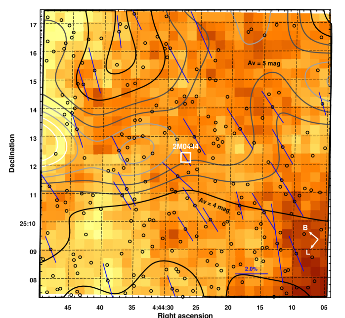
Figure 5: Map of ¹³CO line-integrated emission and extinction A_V across the 2M0444 field. The color image shows ¹³CO integrated emission, from Narayanan et al. (2008), ranging from about 0.3 K km s^-1 for the lightest yellow colors up to about 2.2 K km s^-1 for the darkest colors, near the bottom right corner. The contours indicate inferred A_V values, at about 2 arcmin resolution. Contours trace 3.5 to 7 mag of A_V, in 0.5 mag steps. Lowest extinctions are shown by the black contours, intermediate by gray contours, and highest by the white contours. The positions of the objects used to generate the A_V image are indicated by black circles. The 2M0444 BD is shown by the labeled white box.

A similar map for the 2M0444 field is shown as Figure 5. The background color image is the integrated intensity of ¹³CO, displayed from 0.3 to 2.2 K km s^-1. The contours indicate levels of extinction A_V, from 3.5 to 7 mag. The CO gas and the extincting dust show some correlation, but not as strongly as for the CFHT Tau 4 field. The open black circles show the locations of the 233 objects sampled for reddening, with 195 yielding $(H-M)$ colors from the Mimir observations and WISE and another 38 coming from $(K-M)$ from UKIDSS and WISE, suitably scaled as was done for the CFHT Tau 4 field. The BD 2M0444 was excluded from the A_V determinations.

Extinction along the direction to 2M0444 is of the order of A${}_{V}\sim 5$ mag, based on the extinctions shown by objects in the vicinity that exhibit similar polarization properties. The deduced value of zero mag by Bouy et al. (2008), and cited by Rilinger et al. (2019), would have a low probability of producing the polarization seen for 2M0444, so that null extinction value is judged to be suspect.

3.3 Brown Dwarf and YSO Locations

In Figure 4, the ITG 15 and ITG 17 systems are located on the sky about halfway between the highest column density peak and regions of least extinction in the field. If this YSO and BD were located in front of the HCl2 dust cloud, they should exhibit extinctions (corrected for their disk NIR excesses) less than those predicted for their positions, which are based on the background objects probing the dust layer. If the ITG 15 and ITG 17 systems are located within the HCl2 dust cloud, their extinctions should be comparable to, but perhaps not quite as great as, the background star predicted values. Finally, if the YSO and BD are far behind HCl2, their extinctions should be close to the predicted extinction values for the dust as probed by the background objects.

However, the observed $(H-M)$ colors of the BDs and YSOs are combinations of foreground extinction and the infrared excess in their SEDs, primarily produced by their disks (e.g., Andrews et al., 2013, also see Figure 13 in Appendix C.1 here). For the objects that had their SEDs modeled in enough detail to separate these two reddening components, namely the BDs ITG 17 and 2M0444 and the YSOs ITG 15 and ITG 25, comparison to the cloud extinctions is straightforward. The objects that lack such detailed SED modeling represent an additional challenge, as followed in Appendix A.

Table 3 summarizes, for the two BDs and the two YSOs, the observed (A${}_{V_{O}}$), interpolated (A${}_{V_{I}}$), and modeled (A${}_{V_{M}}$) values of A_V and introduces two ratios to aid location determinations. Column (2) lists the A${}_{V_{I}}$ values found to be present along the directions to the target objects in the interpolated A_V images, shown as Figure 4 and Figure 5. The A${}_{V_{O}}$ values estimated directly from the observed $(H-M)$ values for the objects are listed in column (3), where $H$-band is from the Mimir observations and the $M$-band is from WISE W2-band photometry. The ¹³CO integrated intensity along the direction including each listed object is presented in column (4). While there is a weak correlation of this quantity with the interpolated A${}_{V_{I}}$ values, the dynamic range of the ¹³CO is limited, likely as a result of a combination of optical depth effects and freeze-out of that molecular tracer onto dust grains for the greater extinction lines of sight. The A${}_{V_{M}}$ values obtained through SED modeling of the four objects by Andrews et al. (2013), Bouy et al. (2008), Zhang et al. (2018), and Ward-Duong et al. (2018) are listed in column (5). These values are in good agreement for ITG 15 and ITG 17 but differ for ITG 25 and 2M0444. In the following analyses, the Andrews et al. (2013) A${}_{V_{M}}$ values were adopted.

Two ratios of A_V values were created, as listed in columns (6) and (7) of Table 3. The first, $R_{1}$, is the ratio of the SED-modeled A${}_{V_{M}}$ for an object (column (5)) to the locally interpolated A${}_{V_{I}}$ value through HCl2 (column (2)) along the same direction. The second, $R_{2}$, is the ratio of the observed $(H-M)$-based A${}_{V_{O}}$ value for the object (column (3)) to the interpolated A${}_{V_{I}}$ value (column (2)).

Table 3: Dust Extinctions - Interpolated, Observed, and Modeled

Desig.	A${}_{V_{I}}$	A${}_{V_{O}}$	13CO Integrated	A${}_{V_{M}}$	$R_{1}$	$R_{2}$
	Interpolated	Observed	Intensity	Modeled	((5)/(2))	((3)/(2))
	(mag)	(mag)	(K km s-1)	(mag)
(1)	(2)	(3)	(4)	(5)	(6)	(7)
ITG 15	10.1	11.8	3.5	4.16$\pm$0.54a	0.41$\pm$0.05	1.17$\pm$0.04
				4.35$\pm$0.85b
				0.5c
ITG 17	10.6	16.2	3.8	5.67$\pm$0.89a	0.53$\pm$0.08	1.53$\pm$0.04
				6.37$\pm$0.85b
ITG 25	13.0	23.8	4.1	10.65$\pm$0.75a	0.82$\pm$0.06	1.83$\pm$0.03
				2.6$\pm$4.0b
2M0444	5.1	11.3	1.3	2.05$\pm$1.12a	0.40$\pm$0.22	2.22$\pm$0.09
				0.0d	0.0

Note. — Uncertainties are about 0.1 mag for column (2), 0.4 mag for column (3), and 0.1 K km s^-1 for column (4). References: ^a Andrews et al. (2013), ^b Zhang et al. (2018), ^c Ward-Duong et al. (2018), ^d Bouy et al. (2008)

If all of the objects providing $(H-M)$ values were located behind the extincting and polarizing dust material associated with HCl2 and none of those objects exhibited infrared excess emission, then the corresponding $R_{2}$ values computed for those objects should all be near unity. Some spread of $R_{2}$ values could result due to extinction variations across the fields of view being only partially captured by the 2 arcmin resolution of the interpolations used. The $R_{2}$ distribution for each field was developed from the $(H-M)$ values for all objects indicated in Figures 4 and 5 as black circles, again holding aside the ITG and 2M0444 objects. For each $(H-M)$ value, the propagated uncertainties were used to create gaussian probability distributions that were normalized and accumulated. This yielded more representative net probability distributions, though low SNR objects contribute distribution broadening.

The resulting distributions for the two fields were similar enough that the area normalized distributions were averaged and are plotted as the solid black curve in Figure 6. There, the left side vertical axis shows the probability density, as the base-2 log, and the horizontal axis represents $R$ values (both $R_{1}$ and $R_{2}$ are plotted using the same horizontal axis), also in base-2 log form. The dashed black line displays the cumulative probability for the $R_{2}$ values for the two fields, referenced to the right side linear vertical axis. The 50% cumulative probability for objects in both fields occurs at an $R_{2}$ value of 0.98, with 16% and 84% cumulative probabilities found at $R_{2}$ values of 0.62 and 1.65.

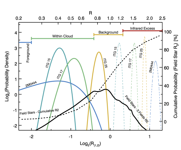
Figure 6: Probability distribution functions for A_V ratio functions $R_{1}$ ($\equiv$ A${}_{V_{M}}$ / A${}_{V_{I}}$) and $R_{2}$ ($\equiv$ A${}_{V_{O}}$ / A${}_{V_{I}}$). Horizontal axis displays the $R$ value, as base-2 log values. Left side vertical axis is the base-2 log of the probability density. Right side scale is linear cumulative probability percentage. The solid black curve displays the $R_{2}$ probability density for the background objects in the two observed fields, as described in the text. The dashed black curve is the corresponding cumulative $R_{2}$ probability. Solid colored curves display $R_{1}$ probability densities for 2M0444 (blue), ITG 15 (teal), ITG 17 (green), and ITG 25 (yellow). Dashed colored curves display $R_{2}$ probability densities. Labeled horizontal colored lines across the top indicate approximate location predictions with respect to HCl2. All four of the target objects are judged to be embedded within HCl2.

For the set of background objects used to create the interpolated A_V images and contours, the integrated $R_{2}$ likelihood below 0.25 is less than 5%. Values of $R_{2}$ this low, or lower, would be expected for nearly all bona fide foreground objects, as the extinction in the diffuse ISM foreground to HCl2 is expected to be nearly negligible. A value for this inner cloud boundary of less than 0.25 could have been chosen instead, but that might have caused foreground stars to be misclassified as embedded due to photometric uncertainties or small-scale cloud structure variations.

Objects embedded within HCl2 would not be expected to suffer the full line-of-sight extinction seen to bona fide background objects. Objects with $R_{2}$ values greater than the 0.25 inner boundary but still less than about unity could be deemed embedded. A rough outer cloud limit of 0.75 for $R_{2}$ was judged to represent a fair compromise that accommodated expected cloud structure and photometric variations in a spirit similar to the choice for the inner boundary. Objects with $R_{2}$ values well beyond unity are surely background to HCl2 with one significant exception. Objects with disks or envelopes have SEDs featuring emission from those dusty components in excess of that expected of their central object photospheres. These infrared excesses are a hallmark of BDs and YSOs with disks (and/or envelopes) and objects showing such excesses should not immediately be interpreted under the $R_{2}$ formalism as being located behind HCl2.

Figure 6 displays the $R_{1}$ and $R_{2}$ information for the three ITG objects and 2M0444 as solid probability density curves for their $R_{1}$ values and as dashed curves for their $R_{2}$ values. Labeled solid lines across the top of the Figure indicate the approximate location assignment zones.

The $R_{1}$ curves for ITG 15, ITG 17, and 2M0444 lead to their classifications as being embedded within HCl2. The ITG 25 SED-modeled extinction places this object on the boundary between being embedded and being considered background. However, it is unlikely to be far in the background, given that its parallax and proper motions match the other objects in cluster 14 of HCl2 (Galli et al., 2019, and Figure 3 here). Note that the $R_{2}$ (dashed colored) curves, which ignore the SED-apportionment of A_V, for these same four objects in Figure 6 all exhibit infrared excesses, as was expected for these disk-containing systems.

While there is a small chance that ITG 15 and ITG 17 are located just in front of HCl2 and so do not partake of the polarization impressed on starlight by HCl2, it is far more likely that both systems are embedded within HCl2 and that their light is affected by the magnetic field and dust in HCl2. The SED modeling by both Andrews et al. (2013) and Zhang et al. (2018) return A${}_{V_{M}}$ values of 4–6 for these objects, effectively excluding foreground or cloud front surface locations.

3.4 Magnetic Field Polarization Properties of Heiles Cloud 2

Having established that the BDs ITG 17 and 2M0444, along with the YSOs ITG 15 and ITG 25, are embedded within HCl2, the next step is to determine the polarization properties impressed on their starlight by HCl2. Doing so will allow those properties to be removed from the measured polarization signals of these target objects and so reveal the intrinsic polarization properties associated with the BD and YSO disks.

Gaia distances alone cannot provide the information sought, as the front and back locations of HCl2 along the directions sampled cannot be resolved with the angular and distance resolutions needed. Instead, a process that uses the relative extinctions developed in the previous section was developed and applied.

3.4.1 Stokes $U$ and $Q$ maps

Maps of the observed Stokes parameters were created to allow characterizing and correcting for the HCl2 polarization contributions. The methodology was the same as used to create Figures 4 and 5, from the $(H-M)$ values. Described in Clemens et al. (2016), the software forms interpolated maps of Stokes $U$ and Stokes $Q$ using all of the measured values, applying gaussian weighting by offset from each object to each map pixel and variance weighting by Stokes parameter uncertainties. Because of the gaussian nature of the Stokes parameters and the variance weighting, using all of the observed values, including polarization upper limits, increases information and angular resolution with little increased noise. The BDs and YSOs were excluded from the interpolation input data sets, so that correction by the resulting Stokes maps, using values interpolated to the positions of the BDs and YSOs, could be performed as was done for the A_V maps.

In the CFHT Tau 4 field, 118 objects that were not the designated targets had Stokes parameter information measured using Mimir in the $H$-band. For a $10\times 10$ arcsec grid of synthetic pixel positions across the observed Mimir field, all non-target objects within 4 arcmin offset were sampled for their Stokes $U$ and $Q$ values, with weighting by the variance of those quantities and weighting by a gaussian of offset of each object from the grid position. For the CFHT Tau 4 field, an offset weighting gaussian with full width at half maximum (FWHM) of 4 arcmin provided adequate numbers of objects for each grid position and yielded good SNR for the predicted Stokes parameters at the positions of the ITG objects. Smaller FWHM values resulted in poorer map coverage and higher predicted uncertainties for the Stokes parameters. Greater FWHM values would result in smaller uncertainties in the predicted Stokes values, with use of the all of the data to compute a full-field weighted average representing the extreme application of this approach. But, in Figure 2, there appear to be bona fide differences in the polarization properties of HCl2 across the CFHT Tau 4 field that need to be included in the Stokes accounting if accurate values for the BD and YSO disk polarizations were to be achieved, hence 4 arcmin seemed to be a useful compromise resolution.

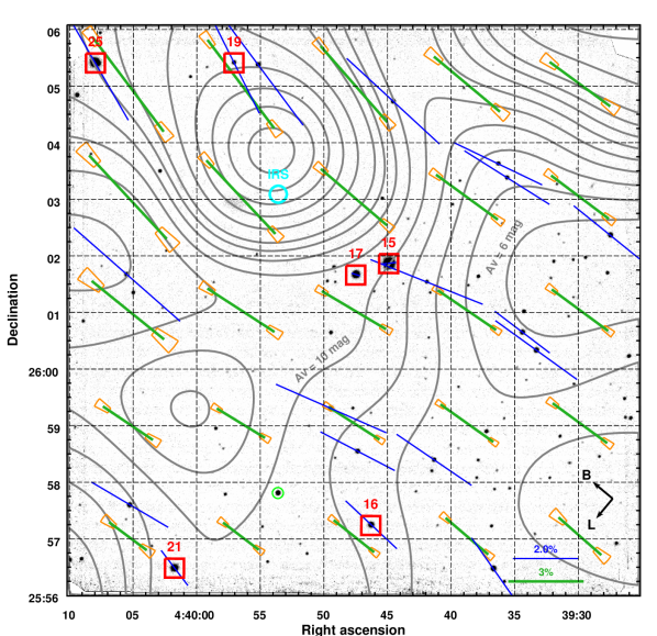
Figure 7: Synthetic polarization pattern derived from the HCl2 Stokes $U$ and $Q$ interpolations for the CFHT Tau 4 field. The background Mimir $H$-band image, blue lines, and red boxes are the same as in Figure 2. Contours and contour labels are the same as in Figure 4, though all contours are colored gray here. Green pseudo-vector lines display interpolated $P^{\prime}_{I}$ and EPA_I values on a Nyquist-sampled grid, spaced at half of the 4 arcmin FWHM resolution. Orange torus segments at the ends of the green lines indicate $\pm$2$\sigma$ uncertainties in $P^{\prime}_{I}$ and EPA_I, as described in the text. Significant changes in $P^{\prime}_{I}$ and EPA_I are evident across the field as the changing lengths and orientations of the green lines.

Figure 7 presents synthetic polarization information for the CFHT Tau 4 field, computed from the interpolated Stokes $U$ and $Q$ arrays as a Nyquist-sampled ($2\times 2$ arcmin) grid of values. The resulting 25 pseudo-vectors display the interpolated debiased polarization percentage $P^{\prime}_{I}$ and equatorial polarization position angle EPA_I via their lengths and orientations. The $\pm 2$ $\sigma$ uncertainties for $P^{\prime}_{I}$ and EPA_I are encoded in the orange torus segments at the ends of each green pseudo-vector. Thus, for each synthetic pseudo-vector, there is a 90% likelihood that the pseudo-vector ends are constrained to lie within the orange uncertainty torus segments.

For the 2M0444 field, there were 275 non-target objects available, more than twice as many as in the CFHT Tau 4 field, enabling use of FWHM resolutions smaller than 4 arcmin. In this field, 2 arcmin still produced low SNR values and 4 arcmin missed some of the smaller-scale changes revealed at 3 arcmin, so this latter value was chosen as the best value.

3.5 Foreground Stokes Parameters Correction Methods

Correcting the observed target polarization values by the interpolated Stokes parameters across each Mimir field could follow any of three methods. The first, and simplest, approach would be to directly subtract the interpolated Stokes parameters at the positions of the target stars from the observed Stokes parameters for each target, to obtain residuals that represent the intrinsic NIR polarization of the BD or YSO systems. The drawback to this bulk correction approach is that the contaminating polarization signal contributed by HCl2 might depend on the depth of the target systems within the cloud. A YSO on the back side of the cloud would suffer nearly all of the contamination provided by the intervening cloud while a YSO close to the near side of the cloud would not. Hence, a second approach would be to scale the background starlight determined Stokes parameters by the extinction to the target system relative to the full extinction through the cloud in that direction. This scaling factor would be the $R_{1}$ ratio described earlier. However, this approach, though an improvement over the simpler one, fails to recognize that polarization and extinction contributions are not linearly related in dark molecular clouds.

The third approach adopted here is based on a determination of how polarization scales with extinction for each of the observed fields and extends that to an illuminated slab model to estimate the best apportioned Stokes parameters to use as foreground corrections, as described in the following section.

Alternate approaches also exist that would take into account the clumpy, turbulent, or fractal nature of molecular clouds and might also account for small-scale local cloud core density enhancements, usually associated with star forming regions but perhaps still present here after these BDs and YSOs moved into their Class II phases. Unfortunately, none of these methods have any background stellar polarimetry observations to guide or constrain them, leaving them in the realm of speculation for now.

3.5.1 Polarization Efficiency Dependence on Extinction

The dust grains responsible for extinction and polarization are generally considered well-mixed, if not identical. But, were this strictly the case, observed polarization percentages $P^{\prime}_{O}$ should rise linearly with observed extinctions A${}_{V_{O}}$. Such linear behavior would cause polarization efficiency (PE $\equiv P^{\prime}_{O}$/A${}_{V_{O}}$) to be independent of A${}_{V_{O}}$. An opposite view is that dust grains align to magnetic fields only in the outer portions of molecular clouds and either the magnetic fields are excluded from cloud interiors or dust grains do not align to any magnetic fields located there (e.g., Goodman et al., 1995; Arce et al., 1998). In this case, PE is high at low extinctions but should decrease as A${}_{V_{O}}^{-1}$ for higher extinctions. This would yield a power law index of $-1$ in a PE versus A${}_{V_{O}}$ plot.

In practice, neither flat nor $-1$ slopes are seen, with observed indices ranging from about $-0.5$ to $-0.9$ (Andersson et al., 2015; Pattle et al., 2019). This has been interpreted to indicate that although dust grain alignment efficiency does decrease with optical depth into molecular clouds, magnetic fields are still detected via dust grain alignment, though with less alignment efficiency at higher extinctions. This has been most readily explained by the micro-physical model of radiative aligned torques (RATS; c.f., Lazarian & Hoang, 2007; Andersson et al., 2015) for dust grains.

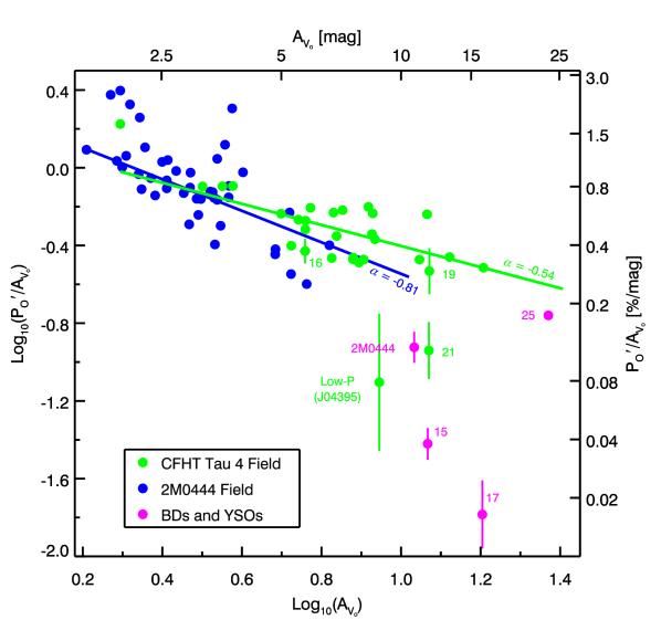
Figure 8: Comparison of apparent (observed) polarization efficiency (PE = $P^{\prime}_{O}$ / A${}_{V_{O}}$) versus extinction A${}_{V_{O}}$ for objects in the two fields, in log-log form. Blue points represent objects in the 2M0444 field and green points are for objects in the CFHT Tau 4 field. Lines in those same colors represent power law fits, with indices $\alpha$ shown near each line. Both show slopes that are shallower than $-1$ and steeper than zero. Magenta points are the three ITG objects plus 2M0444. The green numbered ITG stars are discussed in Appendix A. The green filled circle labeled ‘Low-P’ is the same object indicated by a green circle in Figure 2 and is discussed in Appendix C.

Figure 8 displays PE versus A${}_{V_{O}}$ for the objects in the two fields observed here, color coded as indicated in the inset legend. The objects appearing in this plot all met five selection criteria: $\sigma_{EPA}<28.65\arcdeg$ (i.e., $P^{\prime}/\sigma_{P}>1$); $\sigma_{(H-M)}<0.3$ mag (where $m_{H}$ was from the Mimir observations and $m_{M}$ was from WISE); $\sigma_{P}<2$%; (A${}_{V}/\sigma_{A_{V}})>1$ (where A${}_{V}=7.6$ ($H-M-0.08$) mag; Majewski et al., 2011); and (PE $/\sigma_{PE})>1$. The target BDs and YSOs were excluded from the power law fits, and the fits were weighted by the propagated $\sigma_{PE}$ variances. The 2M0444 field shows a fairly steep PE versus A${}_{V_{O}}$ slope of $-0.81\pm 0.15$. The more extincted CFHT Tau 4 field shows a shallower $-0.54\pm 0.11$ slope, indicating a weaker loss of PE with optical depth than seen in the other field, even though the CFHT Tau 4 field was probed to higher A${}_{V_{O}}$. This could indicate different intensities or SEDs of the external illumination for the two fields, different dust size distributions in the fields, or some combination of both sets of effects.

Examination of Figure 8 leads to a first conclusion that PE in these fields is not independent of A${}_{V_{O}}$ (slope is not zero) nor does $P^{\prime}_{O}$ exist only at the cloud surface (slope is not $-1$). A second conclusion is that the locations of ITG 16 and ITG 19 close to the green line in Figure 8 are consistent with their assignments as normal background objects and not embedded YSOs (see Appendix A). ITG 15, ITG 17, ITG 25, and 2M0444 all exhibit much lower polarization percentages for their apparent ($H-M$)-based A${}_{V_{O}}$ values, compared to normal background objects. As much of the apparent reddening for these objects is due to thermal emission from their warm disks, some portion of their PE departures is due to this effect. However, they also show weaker observed polarizations due to their intrinsic (disk) polarizations being diminished by passage through the magnetized HCl2 material. The green circled labeled ‘Low-P’ identifies a star with a lower polarization percentage ($P^{\prime}_{O}$ $=0.69\pm 0.56$%) than objects of similar brightness in the CFHT Tau 4 field. Its nature is examined in Appendix C.

The decay of PE with A_V may be interpreted under the RATs paradigm as loss of the radiation needed to spin up dust grains deeper in the cloud interior, with the assumption that the radiation arises outside of the cloud. If the illuminating radiation arrives to one side of the cloud, only, then the power laws of Figure 8, with indices $\alpha$, maybe inverted to predict polarization fractions $P$ that scale like A${}_{V}^{\alpha+1}$.

For HCl2, there is no obvious illuminator providing such anisotropic radiation, so a more likely model is one where the Diffuse Galactic Light (e.g., Brandt & Draine, 2012) or the Interstellar Radiation Field (e.g., Mathis et al., 1983) illuminates the cloud from both front and back sides. The model of a slab immersed in two-sided uniform illumination yields a functional form for $P(A_{V})$ that changes strongly at both surfaces and less strongly in the central portion of the cloud. Under this model, the foreground cloud polarization that is added to the target intrinsic polarization will depend on depth of the target into the cloud as:

$$P/P_{max}=0.5\ \{1+R_{1}^{(\alpha+1)}-(1-R_{1})^{(\alpha+1)}\},$$ (1)

where $P/P_{max}$ is the fractional polarization signal contributed, relative to the maximum along that line of sight, and $R_{1}$ is the similar ratio of the extinction A_V to the target, relative to the maximum extinction along the line of sight.

Figure 9 presents the Eq 1 curves for the $\alpha$ values displayed in Figure 8 for the two observed fields. The thicker green and blue curves show the behavior for $\alpha=-0.54$ (the CFHT Tau 4 field) and $\alpha=-0.81$ (the 2M0444 field). Thinner curves flanking the thick curves show the behavior for $\alpha$ values offset by $\pm 1\sigma$ from nominal. Values of $R_{1}$ less than zero and beyond unity are assumed to produce no foreground cloud polarization and full foreground cloud polarization, respectively.

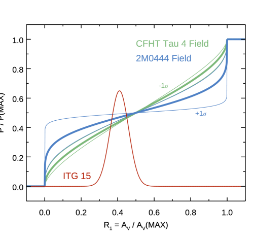
Figure 9: Plot of normalized polarization percentage contributed to the starlight of an embedded target versus normalized visual extinction to the target into the cloud, $R_{1}$. Thick green curve shows the behavior of Eq 1 for the CFHT Tau 4 star field, derived from the power law fit shown in Figure 8. Thinner green curves show the behavior for slope values ($\alpha$) that are offset from nominal by the uncertainty in the fitted slope. Blue thick and thin curves show the similar behaviors for the 2M0444 field. Red curve shows a gaussian representation of the $R_{1}$ value and uncertainty listed for ITG 15 in Table 3. The effective correction factors for the Stokes $U$ and $Q$ values were found from the integrated overlap of the ITG 15 curve with one of the green curves representing the PE behavior for the field containing that star, as described in the text.

To develop the best estimates of the HCl2 contributed foreground polarization for each of the four target systems, a Monte Carlo simulation was employed. For each target system, it started with the appropriate slope for the observed field and added gaussian deviates scaled by the uncertainty in the slope to produce a trial slope. The A_V likelihood function for each target was taken as a gaussian with the mean and width as listed for the value and uncertainty of $R_{1}$ in Table 3 (and as displayed in Figure 9). The $P(A_{V})$ curve was integrated with the A_V likelihood as a kernel to yield one $P/P_{max}$ value. The loop of selecting another trial slope to yield a new $P/P_{max}$ value was repeated to develop a distribution function for that ratio, and afterwards characterized as a mean and standard deviation for the ratio.

The Stokes $U$ and $Q$ parameters were assumed to follow the behavior of the polarization with extinction, such that the apportioned foreground HCl2 contributed Stokes $U_{F}$ was formed as the product of the $P/P_{max}$ ratio and the full interpolated background star Stokes $U_{I}$, and similarly to create $Q_{F}$. The similarly scaled interpolated background star Stokes parameter uncertainties were added in quadrature with the dispersion of the $P/P_{max}$ probability function to yield final uncertainties for $U_{F}$ and $Q_{F}$.

3.5.2 Applying the Foreground Corrections

These apportioned foreground Stokes parameters were subtracted from the observed Stokes parameters for a particular target system to yield residuals ($Q_{R}$, $U_{R}$), and uncertainties were propagated. These residual values represent the current best estimates for the intrinsic Stokes parameters of each of the target YSO and BD systems, without contamination from the HCl2 contributions.

This foreground correction process is summarized in Table 4, which lists for each of the objects: the observed Stokes parameters ($Q_{O}$, $U_{O}$); the Stokes parameters estimated from the interpolation of the background star values across each of the fields of view at the positions of each of the BDs and YSOs ($Q_{I}$, $U_{I}$); the Stokes parameters apportioned to the foreground of each object, using the analysis based on Eq 1, ($Q_{F}$, $U_{F}$); and the residual differences of the observed and apportioned foreground sets of values ($U_{R}$, $Q_{R}$) that reveal the intrinsic NIR polarization of the YSO and BD systems.

Table 4: Stokes Parameters: Observed, HCl2 Foregrounds, and Residuals

Desig.	Quantities	Stokes $Q$	Stokes $U$	$P$	$\sigma_{P}$	$P^{\prime}$	EPA
		(%)	(%)	(%)	(%)	(%)	(°)
(1)	(2)	(3)	(4)	(5)	(6)	(7)	(8)
ITG 15	A: Observed ($X_{O}$)a	$-$0.44$\pm$0.08	$-$0.10$\pm$0.08	0.45	0.08	0.44	96.2$\pm$5.4
	B: Interpolated Background ($X_{I}$)	$-$1.22$\pm$0.24	$+2.82\pm$0.25	3.07	0.25	3.06	56.7$\pm$2.2
	C: Apportioned Foreground ($X_{F}$)	$-$0.54$\pm$0.11	+1.24$\pm$0.11	1.35	0.11	1.35	56.8$\pm$2.3
	D: Residuals (Intrinsic = A - C) ($X_{R}$)	+0.10$\pm$0.14	$-$1.34$\pm$0.13	1.34	0.13	1.34	137.0$\pm$2.8
	E: PA Difference (= D - B) ($X_{D}$)						80.2$\pm$3.6
ITG 17	A: Observed ($X_{O}$)	$-$0.24$\pm$0.11	+0.16$\pm$0.11	0.29	0.11	0.26	73.0$\pm$11.5
	B: Interpolated Background ($X_{I}$)	$-1.31\pm 0.27$	$+2.83\pm 0.26$	3.12	0.26	3.11	57.4$\pm$2.3
	C: Apportioned Foreground ($X_{F}$)	$-$0.68$\pm$0.14	+1.47$\pm$0.14	1.62	0.14	1.61	57.4$\pm$2.5
	D: Residuals (Intrinsic = A - C) ($X_{R}$)	+1.08$\pm$0.29	$-$2.67$\pm$0.28	2.88	0.28	2.87	146.0$\pm$2.7
	E: PA Difference (= D - B) ($X_{D}$)						88.6$\pm$3.7
	F: ALMA						25$\pm$5b
							40$\pm$10c
ITG 25	A: Observed ($X_{O}$)	+2.04$\pm$0.10	+3.53$\pm$0.10	4.08	0.10	4.08	30.0$\pm$0.7
	B: Interpolated Background ($X_{I}$)	$+1.41\pm 0.42$	$+4.68\pm 0.42$	4.89	0.42	4.87	36.6$\pm$2.4
	C: Apportioned Foreground ($X_{F}$)	+1.03$\pm$0.31	+3.42$\pm$0.34	3.57	0.33	3.55	36.6$\pm$2.7
	D: Residuals (Intrinsic = A - C) ($X_{R}$)	+1.01$\pm$0.33	0.11$\pm$0.35	1.02	0.34	0.96	3.0$\pm$10.1
	E: PA Difference (= D - B) ($X_{D}$)						146.4$\pm$10.5
2M0444	A: Observed ($X_{O}$)	+0.51$\pm$0.23	+1.21$\pm$0.24	1.31	0.24	1.29	33.6$\pm$5.3
	B: Interpolated Background ($X_{I}$)	$+0.96\pm 0.10$	$+1.80\pm 0.10$	2.04	0.10	2.04	31.0$\pm$1.4
	C: Apportioned Foreground ($X_{F}$)	+0.43$\pm$0.05	+0.81$\pm$0.05	0.92	0.05	0.92	31.0$\pm$1.6
	D: Residuals (Intrinsic = A - C) ($X_{R}$)	+0.08$\pm$0.23	+0.40$\pm$0.25	0.41	0.24	0.33	39.5$\pm$20.8
	E: PA Difference (= D - B) ($X_{D}$)						8.5$\pm$20.9
	F: ALMA						115$\pm$15b
							70$\pm$10c

Note. — References: ^a Indicator of subscript label for all row quantities, ^b Ricci et al. (2014), ^c Rilinger et al. (2019)

The process steps for the ITG 15 object began with the first (A) row for that object in Table 4 which lists the observed Stokes parameters and the polarization parameters derived from them, all with implied “O” subscripts as noted. Those observed $H$-band Stokes $Q_{O}$ and $U_{O}$ were $-0.44\%\pm 0.08$% and $-0.10\%\pm 0.08$%, respectively. The second (B) row lists the interpolated values for Stokes $Q_{I}$ and $U_{I}$ at the position of ITG 15 as $-1.22\%\pm 0.24$% and $+2.82\%\pm 0.25$%, respectively. The third (C) row lists the Eq 1 apportionment of the B-row values to yield the HCl2 foreground corrections of $-0.54\%\pm 0.11\%$ and $+1.24\%\pm 0.11\%$ for $Q_{F}$ and $U_{F}$, respectively. Subtracting these from the observed values produced the (D) row of residuals with Stokes $Q_{R}$ and $U_{R}$ values of $+0.10\%\pm 0.14$% and $-1.34\%\pm 0.13$%, respectively. From each of these four sets of Stokes $Q$ and $U$ values, the derived quantities $P$, $\sigma_{P}$, $P^{\prime}$ , EPA, and $\sigma_{EPA}$ were developed, and are listed in columns (5) through (8) of the (A)-(D) rows for each object in Table 4. Note that once corrected for the apportioned Stokes foreground $Q_{I}$ and $U_{I}$ contributions due to the passage of light through HCl2, the residual debiased polarization percentage $P^{\prime}_{R}$ for ITG 15 rose to $1.34\%\pm 0.13$% from the observed $P^{\prime}_{O}$ value of $0.44\%\pm 0.08$%.

Similarly, the observed polarization EPA_O (in row A) for ITG 15 changed from $96\arcdeg.2\pm 5\arcdeg.4$ to an EPA_R of $137\arcdeg.0\pm 2\arcdeg.8$ upon correction for the HCl2 contributions. The interpolated EPA_I (in row B) is a direct measure of the plane of sky magnetic field orientation for HCl2, so it can also be compared to the residual EPA_R (in row D) to assess any relationship of the intrinsic polarization of this BD disk system to the ambient magnetic field. That EPA_D difference (EPA_R - EPA_I) is listed in the (E) row for ITG 15 as $80\arcdeg.2\pm 3\arcdeg.6$, which is close to being perpendicular.

The Table 4 entries for the remaining three BD and YSO objects follow the same order of processing steps and comparisons to their ambient magnetic field orientations. For the two BDs, ITG 17 and 2M0444, the EPAs of ALMA-traced dust disk orientations were determined by Ricci et al. (2014) and Rilinger et al. (2019) and are listed in the (F) rows.

Changing the angular resolution of the interpolated HCl2 Stokes maps had only minor effects on the residuals listed in the (D) rows for each object in Table 4. Such changes tended to be at or below the 1 $\sigma$ level for EPA_R and much less than 1 $\sigma$ for $P^{\prime}_{R}$ values when the interpolation resolution was changed by $\pm$1 arcmin FWHM, for example. Thus, the residual values are robust against the interpolation resolution chosen.

3.6 Intrinsic Near-Infrared Polarization of Brown Dwarf and YSO Disks

The debiased polarization percentage residuals for one of the two BDs (ITG 17) and both of the YSOs are all significant at, or beyond, the 2.8 $\sigma$ level while the other BD (2M0444) has only a $1.4\sigma$ residual. These residuals represent the current best estimate of the polarization emitted from these systems prior to that radiation being modified by the magnetized dust within HCl2. Hence, these residuals are the polarization properties of the light arising from the photospheres and disks of each of these systems. In three of the four cases, significant polarization was found, which is highly unlikely to arise in their photospheres and so must arise from their disks (none of the four systems exhibit envelope emission in their SEDs; Andrews et al. 2013).

Figure 10 shows a zoomed portion of the CFHT Tau 4 field presented in Figure 2. This portion includes both of the ITG 15AB and ITG 17AB systems and shows where other studies located the faint (B) possible companions (Table 1). The blue pseudo-vector lines indicate the observed NIR polarization $P^{\prime}_{O}$ and EPA_O values for the primary (A) objects. The dashed black line shows the orientation of the mean interpolated polarization EPA_I for this region, i.e., the magnetic field orientation in this portion of HCl2.

The EPAs observed for ITG 17 (EPA_O) and for HCl2 (EPA_I) differ by only $16\arcdeg\pm 12$°, implying similarity, but their fractional polarizations $P^{\prime}_{O}$ and $P^{\prime}_{I}$ differ by $3.0\%\pm 0.4$%, which is significant. ITG 15 shows a greater EPA deviation (EPA_O - EPA_I) from that of HCl2 in this region, namely $39\arcdeg\pm 6$° and a polarization fraction difference ($P^{\prime}_{O}$ - $P^{\prime}_{I}$ = $2.6\pm 0.3$%) nearly as large as is seen for ITG 17. Thus, the observed polarizations for these objects do not match the polarization created by magnetically-aligned dust grains in HCl2. The light from these two disk systems does have to pass through portions of the HCl2 aligned dust grains, as argued earlier. Correcting for this HCl2 contribution results in the intrinsic (residual) polarization EPA_R values listed in the (D) rows in Table 4 and shown in Figure 10 as the red lines and labels at each of the two objects.

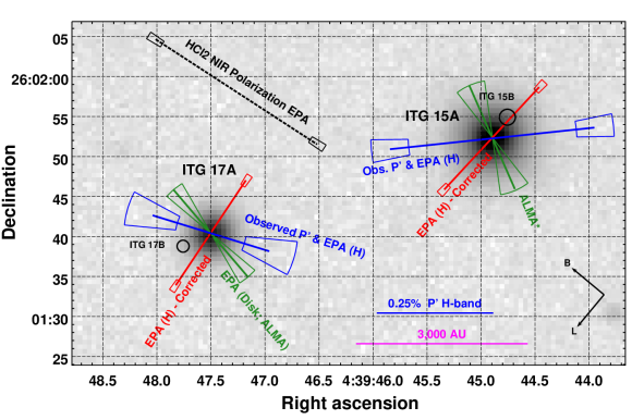
Figure 10: Zoom of the central region of Figure 2, showing the relative locations of ITG 17A and ITG 15A as well as their possible companions ITG 17B and ITG 15B. The $H$-band observed $P^{\prime}_{O}$ and EPA_O values are encoded in the lengths and orientations of the blue lines, with a 0.25% blue reference line shown at lower right. The EPA of the orientation of the elongation of the ITG 17 disk modeled using ALMA continuum imaging analysis by Rilinger et al. (2019) is indicated as the green line. The EPA of the orientation of the ITG 15 disk (labeled ALMA*) deduced from the observations obtained by Ward-Duong et al. (2018) is also shown in green and is described in Section 3.6.1 of the text. After correcting the observed $H$-band Stokes parameters for the foreground HCl2 field polarization, whose average EPA_I orientation is shown as the black dotted line, the intrinsic EPA_R values for ITG 17 and ITG 15 are recovered and are shown as the red lines. Disk rotational angular momenta J would be parallel to these red EPA_R lines and perpendicular to the magnetic field in HCl2, as noted in the text. Uncertainties in $P^{\prime}$ (actual and arbitrarily scaled) and EPA are indicated by the torus segments at the ends of each line, representing $\pm 1\sigma$ ranges. The ALMA line lengths have no meaning, hence their error tori extend to zero length to indicate that the angular uncertainties do have meaning. At 140 pc distance, the projected relative separation of ITG 17A and ITG 15A is about 5,200 au. The projected relative separations of ITG 15A from ITG 15B and ITG 17B from ITG 17A are about 400-600 au.

The red lines in Figure 10 are remarkable for three reasons. First, both are nearly perpendicular to the HCl2 magnetic field EPA_I, as listed in the (E) rows in Table 4. As these intrinsic NIR polarization disk EPA_R values are expected to be parallel to their sky projected disk angular momentum vectors (J) (see Section 4), the local magnetic field B and disk momenta J are apparently perpendicular for both systems. Second, the red lines are parallel to each other, as listed in the (D) rows in Table 4 ($\Delta{\rm PA}=9\arcdeg\pm 4\arcdeg$), indicating that the J vectors for the two disks are aligned (or anti-aligned, as kinematic information is lacking). Finally, the EPA of the elongation of the disk for ITG 17, as modeled for ALMA continuum imaging by Rilinger et al. (2019, namely $40\arcdeg\pm 10$°), is shown as the green line and label in Figure 10. It is $106\arcdeg\pm 10$° from the intrinsic (residual) NIR EPA_R for ITG 17, and so, nearly perpendicular to the NIR EPA_R and thus perpendicular to the inferred J vector. Hence, for ITG 17, both ALMA continuum imaging and NIR polarimetry agree as to the disk orientation. The difference angle grows to 121°, however, if the orientation EPA of the ALMA disk modeled by Ricci et al. (2014) is instead considered.

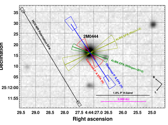
Figure 11: Zoom of the central region of Figure 1 containing the BD 2M0444. In this figure, all NIR polarization vectors are scaled to the black reference at lower right. The NIR polarization direction (EPA_I) and magnitude $P^{\prime}_{I}$ for this direction through HCl2 are indicated by the dashed black line at left. The observed $H$-band polarization is shown as the blue line. The 2M0444 disk $H$-band intrinsic polarization is shown as the red line, which should be perpendicular to the disk elongation direction. Uncertainties in $P^{\prime}$ and EPA are indicated by the torus segments at the ends of each line, representing $\pm 1\sigma$ ranges. The ALMA disk orientations on the sky are indicated by the dark green line for the Rilinger et al. (2019) imaging and by the lighter green line for the Ricci et al. (2014) CO moment determination. Line lengths representing ALMA findings have arbitrary scaling: the angular uncertainties do carry meaning. The NIR inferred disk orientation (EPA_R) is perpendicular to that found by Ricci et al. (2014) from their CO moment map.

A similar comparison of NIR and ALMA findings for 2M0444 is shown as Figure 11. There, the EPA_I of the HCl2 polarization (black dashed line) is seen to be parallel to the observed $H$-band polarization orientation (EPA_O; blue line), but shows a higher fractional polarization ($P^{\prime}_{I}$ versus $P^{\prime}_{O}$). The Stokes differencing results in the red, corrected polarization line that encodes $P^{\prime}_{R}$ and EPA_R in the Figure. The large extents of the red error tori signal the low significance of the NIR residuals, however. The two determinations of the disk orientation from ALMA observations are shown as the dark green line for the Rilinger et al. (2019) resolved continuum imaging and as the lighter green line for the Ricci et al. (2014) CO moment map fitting. The weak apparent agreement of the corrected NIR (red) and ALMA continuum (dark green) orientations actually signals disagreement, as disk elongation is interpreted to be perpendicular to NIR intrinsic polarization. The NIR and Ricci et al. (2014) findings are closer to being perpendicular, with an implied disk orientation difference angle of $76\pm 26$°, only $0.5\sigma$ from 90°, though with high angular uncertainty. The NIR to ALMA continuum difference is $31\pm 29$°, some $2\sigma$ from 90°. Both comparisons are likely too weak to support strong conclusions regarding the disk alignment for 2M0444.

3.6.1 Implications for Disk Orientations

No previously published analysis of ALMA observations of the ITG 15 YSO system provide modeling sufficient to allow direct determination of the dust elongation EPA or gas angular momentum J for its disk. ALMA observations by Ward-Duong et al. (2018) do show a dust detection map, but lack deconvolution to establish disk orientation. Detailed SED fitting by Ballering & Eisner (2019) accounted for inclination but not for disk orientation. Based on the correlation of the intrinsic $H$-band EPA_R values for ITG 15 and ITG 17, and the near perpendicular nature of the ALMA EPA and NIR EPA_R for ITG 17 under the Rilinger et al. (2019) model, a prediction for the ITG 15 dust disk elongation EPA of about $47\arcdeg\pm 3$° can be made.

The ALMA continuum data for ITG 15 system obtained for the Ward-Duong et al. (2018) study were fetched from the ALMA archive. Gaussian fitting after deconvolution by the sampling beam yielded major and minor axes FWHM of $271\pm 35$ mas and $149\pm 45$ mas, respectively, at a position angle of $23\pm 15$° for ITG 15A. The fainter secondary ITG 15B showed deconvolved FWHMs of $369\pm 117$ mas and $105\pm 85$ mas at a position angle of $13\pm 24$°. This new ALMA disk PA is indicted in the Figure 10 zoom image by the ‘ALMA*’ label.

The NIR prediction and ALMA deconvolution differ in their estimated plane of sky disk EPA by $24\pm 15$°  or about 1.6 $\sigma$. Possibly better data might be ALMA spectral line observations that are sufficient to establish the orientation and magnitude of the disk angular momentum J, as was done by Ricci et al. (2014) for 2M0444 (but not for ITG 15).

The ALMA-traced disks about ITG 15A and ITG 17A have PAs that differ by $23\pm 18$°, or only 1.3 $\sigma$ (compared to the even smaller NIR difference of $9\pm 4$°). This seems to indicate that both the NIR intrinsic polarizations and the ALMA continuum observations favor disks about these two systems that are quite similar in sky orientations. The ITG 15A and ITG 15B disks have PAs that differ by $10\pm 28$°, which is too uncertain for strong conclusions.

For the ITG 25 system, though the inferred intrinsic NIR polarization $P^{\prime}_{R}$ is weaker than for the ITG 15 and ITG 17 systems, there is sufficient residual polarization signal to infer the EPA_R orientation of its disk, even though no ALMA observations have determined the disk elongation EPA and no ALMA observations exist in the archive. Analogous to the ITG 17 system, the NIR polarization predicted elongation EPA for ALMA observations of the ITG 25 disk would be about $93\arcdeg\pm 10$°.

4 Discussion

Characterizing the extinctions and polarizations of the many objects background to HCl2, when compared to the measured values for the ITG systems and 2M0444, led to the conclusion that both BDs and both YSOs are located within HCl2. The background star polarizations were used to establish the Stokes parameters contributions resulting from magnetically aligned dust grains within HCl2. Removal of these contributions from the measured Stokes parameters for the embedded systems left residual polarizations that are intrinsic to those systems, most likely resulting from the polarization produced by scattering of photospheric light from disk surfaces.

For a net intrinsic polarization to arise from disk systems, three conditions must be present, none of which are particularly difficult to realize. If the disk is generally symmetric and not dominated by a small number of spiral arms, say, then single scattering of photospheric light by disk surface layer dust will produce a centrosymmetric polarization pattern, with the prevailing electric field vector perpendicular to the radial vector from the central object to the scattering location within the disk (e.g., Silber et al., 2000; Apai et al., 2004). Face-on and nearly face-on disks show just such a pattern (e.g., Potter, 2005; Hales et al., 2006; Follette et al., 2013). However, for an unresolved disk, a face-on presentation has net symmetry in the polarization pattern and will result in low to zero net polarization. Edge-on disks might be expected to extinct scattered light from inner disk surfaces due to high optical depths in thin disks or due to flared outer disk regions. Hence, some inclination of the disk is likely needed in order to detect a net polarization for unresolved NIR observations like those reported here. Finally, the scattering phase function must favor scattering angles near 90° over lesser and greater angle values: such is expected for Rayleigh scattering. Such phase functions have the effect of boosting the polarization signal from the ansae of inclined disks at the expense of the polarization arising from the front or back portions of the disk, though these regions are located closer in projection to the central object than are the ansae. Phase functions favoring 90° scattering have been measured for resolved disks, for example in the nearly edge-on HD 35841 debris disk by Esposito et al. (2018), and show maximum polarization fractions of around 30%.

The combination of some disk inclination, centrosymmetric single scattering from disk surfaces, and phase functions favoring 90° results in net intrinsic NIR polarization for the unresolved disk systems studied here. Further, the relatively high intrinsic polarization fractions for ITG 15 and ITG 17, of about 1-3%, implies that a significant fraction of the photospheric light is intercepted by their disks. The 30% polarization fraction measured by Esposito et al. (2018) in their resolved observations was computed relative to the total light reflected from the same regions, which was a factor of 10-30 times less than that emitted by the HD 35841 central object. That is, if the HD 35841 polarization observations were not spatially resolved, the net system polarization would be more like 1-3%, similar to the values measured here for ITG 15 and ITG 17.

The NIR polarization position angle emergent from an unresolved disk system will be dominated by the ansae reflection polarization favored by the scattering phase function, leading to measured EPA_R values being perpendicular to the elongation axis of the inclined disk and parallel to the sky-projected disk angular momentum vector J. Hence, for the ITG 17 BD system, we expect the intrinsic NIR polarization EPA_R ($146\arcdeg.0\pm 2\arcdeg.7$) to be perpendicular to the elongation EPA found by Rilinger et al. (2019) ($40\arcdeg\pm 10\arcdeg$) from their ALMA analyses and modeling. In Figure 10, the two are very nearly perpendicular ($106\arcdeg\pm 10\arcdeg$), with most of the difference uncertainty arising from the ALMA modeling. Hence, the NIR and ALMA modeling agree as to the disk elongation angle for the BD ITG 17.

The similar comparison for the 2M0444 BD, both between the two ALMA studies and between the ALMA studies and the NIR value found here, was significantly less conclusive due to the weak SNR of the residual NIR polarization, as noted in the previous Section.

Polarization in the NIR could instead arise from shadowing due to warped inner disks causing anisotropic disk illumination (e.g., Benisty et al., 2018). Time-dependent polarization behavior could reveal systems with these properties. A cursory test of the data obtained for this study did not reveal EPA_O changes with time (see Appendix B).

4.1 Aligned Disks in a Wide Binary

The YSO ITG 15 and BD ITG 17 were identified as a possible wide binary system by Joncour et al. (2017, as their couple number 28) and the nature of object clustering within Taurus has been studied by Joncour et al. (2018). Both objects are likely members of the Galli et al. (2019) HCl2 cluster 14 group of about ten objects that spans about 7 cubic parsecs, but these two are the closest pair of objects among all of that cluster, in projection. They are at the same distance (see Figure 3), and if they are in a circular orbit residing purely in the plane of the sky, their orbital period, based on the masses from Table 1, would be about 0.7 million years, similar to their inferred ages. Such an orbit has a predicted relative tangential velocity (0.23 km s^-1) which is similar to the measured relative tangential velocity ($0.45\pm 0.15$ km s^-1) from the Gaia EDR3 reported proper motions of the objects. The projected separation of 5,200 au for the pair is near the limit for M-dwarf wide binaries (Law et al., 2010), but is contained within the central portion of the distribution of ultra-wide pairs for Taurus determined by Joncour et al. (2017). The conclusion is that the possible binaries ITG 15AB and ITG 17AB themselves form a (hierarchical) wide binary (or quadruple system). Additionally, the primaries are somewhat more tightly bound to each other than to the remainder of the cluster 14 group of Galli et al. (2019).

ITG 15B was detected by Gaia in EDR3 (see Figure 3) and in the ALMA observations of Ward-Duong et al. (2018) but ITG 17B has not been reported as detected in ALMA dust continuum observations. As the separations of these companions from their primaries are about 400-600 au, disks would be expected around these systems, based on extrapolation of the statistics for ALMA disks about Class II stars more massive than M6 in Taurus (Akeson et al., 2019) to lower mass objects. If ITG 17B is significantly less massive than its primary and the secondary disk mass scales like the secondary star mass, the ITG 17B disk may be too faint for routine ALMA detection levels. The Akeson et al. (2019) study did not recognize ITG 15 – ITG 17 as a binary in their Class II study of singles, binaries, and multiples, though their summary of the ALMA properties of ITG 15 and ITG 17 in their Table 4, when interpreted as a binary, do exhibit disk masses, disk mask ratios, and disk-to-star mass ratios similar to the other wide binaries (1 - 30 arcsec separation) in their sample.

The parallel EPA_R values for the derived intrinsic $H$-band polarization from these two objects, with a difference EPA of $9\arcdeg\pm 4\arcdeg$ as shown in Figure 10, and the ALMA continuum disk orientation EPA agreements are strong evidence for aligned disks for this hierarchical binary system.

4.2 Brown Dwarf and Disk Formation

Disk and protostar formation appear in modeling studies to be governed by numerous effects and quantities, including ambipolar diffusion, the Hall Effect, Ohmic dissipation, angular momentum and mass transport, infall and outflow, local chemistry, and ionization fractions and rates, as well as grain sizes and distributions (see review by Zhao et al., 2020). None of these quantities is directly available for determination in this study. But, the current disk orientations for ITG 15 and ITG 17, in relation to each other and in relation to the current local mean magnetic field sky projected orientation for HCl2 at or near the location of this binary have been determined. How the apparent orthogonality of B and inferred sky projected J for these disks relates to, constrains, or fails to constrain models of protostellar disk formation and evolution are difficult to discern from this work alone.

A key question is the degree to which present day disk orientations and present day magnetic field orientations can inform physical conditions at the time of formation of the protostars and their disks. For example, although the large-scale magnetic field within HCl2 is unlikely to have changed greatly in orientation and strength over the last 1-2 Myr, magnetic fields in dense cores and protostellar envelopes could be significantly different from the fields in the more diffuse cloud material surrounding the cores. However, the study of solar-mass Class 0 objects and their environs by Galametz et al. (2018) found that “…an ordered B morphology from the cloud to the envelope is observed for most of our objects.” This conclusion of unchanged magnetic field orientations was also reached for the more extended environment from 6,000 au to pc-scales about the low-mass Class 0 protostar GF9-2 by Clemens et al. (2018). Yet a recent study of magnetized filaments in NGC 1333 by Doi et al. (2020) instead finds changes in magnetic field morphologies inside of 1 pc but (complex) morphological continuity between 1 pc and 1000 au. In addition to B-field changes, the disks surrounding ITG 15 and ITG 17 could have changed their projected orientations in their lifetimes. Though for them to appear at the present time in a parallel configuration, after experiencing orientation evolution likely tied to their host star masses, seems unlikely.

Progress may be found in asking which characteristics of the ITG 15 – ITG 17 system could be more easily explained if the current misalignment of the magnetic field and the disks does indicate initial formation conditions. An emerging consensus (review by Zhao et al., 2020, and references therein) is that magnetic fields aligned with disk rotation axes may produce conditions ripe for magnetic braking, leading to weaker disk angular momenta and smaller disk sizes, while misaligned fields may do the opposite, producing disks with stronger angular momenta and larger sizes (e.g., Figure 3 of Galametz et al., 2020), though a recent study in Orion (Yen et al., 2021) finds no disk size correlation with magnetic field misalignment. Turbulence may lead to substantial disks, even for the aligned field case (Gray et al., 2018), indicating that magnetic alignment effects alone may not be sufficient to predict disk or protostar outcomes. Disks with strong angular momenta are also prone to fragmentation (e.g., Wurster & Bate, 2019), leading to binaries or multiple star systems (Zhao et al., 2018; Rosen et al., 2019), many of which retain at least a significant fraction of their individual disk masses (Maury et al., 2019).

In the case of ITG 15 – ITG 17, the binary and aligned disk natures could both be the result of formation in a misaligned magnetic field condition. Indeed, the very wide separation could have had the effect of retaining more disk material, relative to the mass of each host star, than if the stars had less separation. This seems to be born out in the ratio of the secondary (ITG 17A) disk mass to secondary star mass versus the ratio of primary (ITG 15) disk mass to primary star mass, as shown in Figure 12 of Akeson et al. (2019). The ITG 15 – ITG 17 binary exhibits the highest such secondary ratio of all of their binary systems, even for its relatively high primary ratio. The secondary disk is the one about the BD ITG 17, found to be a somewhat large 80 au (Rilinger et al., 2019), which could be explained by a misaligned magnetic field that was present at proto brown dwarf formation and remains so to this day.

4.3 Impacts on Previous Studies

Near-infrared polarimetry has been used in the past to study YSOs and their environs, including in Taurus. For example, Tamura & Sato (1989) examined 39 T Tauri stars for $K$-band (2.2 $\mu$m) polarization, using an aperture polarimeter. They detected linear polarization with a median value of about 0.6% but with polarization position angles that sometimes showed large differences compared to optical polarizations and showed a moderate preference for alignment parallel to local magnetic field orientations. However, Tamura & Sato (1989) did not perform foreground polarization corrections to their observations. Tamura & Sato (1989) argued against the Taurus molecular clouds as the origin of the polarizations they measured, based on mean extinctions and a ratio of $K$-band polarization to extinction, but they did not consider that the intervening material could affect how to use the observed EPA and $P$ values to interpret intrinsic source properties. If the mean $H$-band cloud polarization percentages of about 3-4% (see Table 4) are scaled to $K$-band using an average Serkowski law (e.g., Serkowski et al., 1975), which characterizes the wavelength dependence of polarization, a predicted contribution from the Taurus material of 1-2% in $K$-band is obtained. This exceeds the median $P$ value measured by Tamura & Sato (1989). Hence, a reanalysis of the Tamura & Sato (1989) data to establish the intrinsic polarization for each source would likely find the same sort (and degree) of polarization position angle changes seen here in the $H$-band for the embedded BD and YSO targets. This calls into question the Tamura & Sato (1989) conclusions, and those of other similar studies, that are based on observed EPA or $P$ values but lack corrections for intervening magnetized cloud effects. Tamura & Sato (1989) could not perform these corrections due to the lack of wide-field imaging polarimetric data, hence their findings regarding alignments of disks and outflows are weakened. The novel aspect brought about by the new Mimir observations is the ability to accurately characterize the polarization contributions of the intervening Taurus material to the intrinsic polarization of embedded sources and so allow correction from observed values to the intrinsic ones.

5 Summary

Wide-field near-infrared $H$-band imaging polarimetry observations using Mimir were combined with archival photometry and Gaia EDR3 distance and proper motion information to ascertain the presence of intrinsic linear polarization from two brown dwarf disk systems in Taurus that had previously been analyzed and modeled using archival ALMA data by Rilinger et al. (2019) and two YSO disk systems, all of which are in the direction of the Heiles Cloud 2 (HCl2) dark molecular cloud. Combining the Gaia information with infrared $(H-M)$ colors enabled classifying most of the 400 objects measured for $H$-band polarization as being foreground, embedded, or background to the HCl2 dark molecular cloud. All four target objects were found to be embedded within HCl2 and had significant $H$-band polarizations detected. Background objects were used to ascertain the polarization signals impressed on starlight by HCl2 due to its magnetically aligned dust grains. Correcting the apparent $H$-band polarization values by the HCl2 polarization contributions revealed the intrinsic polarizations of one of the BDs (ITG 17) and both YSO systems, while the remaining BD (2M0444) had low polarization significance after correction.

The NIR polarization-inferred elongation orientation (EPA_R) for the disk around the BD ITG 17, $56\arcdeg\pm 3\arcdeg$, is similar to the ALMA elongation orientation, $40\arcdeg\pm 10\arcdeg$, found by Rilinger et al. (2019). For the BD 2M0444, the corrected NIR polarization yields only a weak comparison with ALMA modeled orientations.

The YSO ITG 15 and the BD ITG 17 likely form a 5,200 au separation M-dwarf wide binary. Both objects show intrinsic disk polarization position angles that are parallel to each other, yet are nearly perpendicular to the local magnetic field orientation within HCl2. This configuration could have arisen from misalignment of an initial magnetic field and the disks at the time of protostar formation. Such misalignment could have also resulted in somewhat larger disk sizes, as is observed for the BD ITG 17.

Using the multiple background stars in the wide Mimir fields to ascertain the polarization induced by HCl2 enabled applying corrections to the brown dwarf and YSO disk system polarizations that led to completely different findings for their intrinsic polarization, and thereby disk, properties as compared to their observed NIR ones. Previous studies that ignored these vital corrections may need to be revisited and their findings reconsidered.

Appendix A The Distant, Non-YSO Natures of Objects ITG 16, 19, and 21

The ITG objects 16, 19, and 21 in the CFHT Tau 4 field were found to be different in nature than the BD ITG 17 and the two YSOs, ITG 15 and ITG 25, in that field. This Appendix summarizes the findings that these three ITG objects are normal, diskless stars located far beyond HCl2 and are not associated with the embedded young objects in that dense molecular cloud.

There are no parallax or proper motion values in Gaia EDR3 for ITG 19 or ITG 21, making their direct distance determinations impossible. ITG 16 is in Gaia EDR3 and exhibits different values for parallax and proper motion than for the BD and two YSOs in the CFHT Tau 4 field, as shown in Figure 3.

All three of these ITG objects lack detailed SED modeling and so have no $(H-M)$ color apportionments between disk-based and foreground extinctions. This leaves only the $R_{2}$ ratio method (see Section 3.3) for locating the objects relative to HCl2. Table 5 lists, for the three ITG objects, the same information as was provided for the BDs and YSOs in Table 3, but absent entries for modeled A${}_{V_{M}}$ or $R_{1}$. The $R_{2}$ values were used to place the corresponding gaussian likelihoods for the objects in Figure 12. It shows the $R_{2}$ distributions for ITG 16 and ITG 19 weakly favor them being within HCl2.

However, as already noted in Section 3.1 and shown in Figure 3, ITG 16 has a Gaia EDR3 parallax value placing it about 1 kpc away, versus the 140 pc distance to HCl2. ITG 16 does not show the extreme IR excesses of the three brighter ITG objects (see Figure 13), and shows polarization properties similar to its other sky neighbors (see Figure 2) which are located at distances well beyond HCl2. Correcting by the apparent reddening and the Gaia parallax, ITG 16 is judged to be a normal red giant and not associated with HCl2.

Although ITG 19 lacks Gaia EDR3 parallax or proper motion values, it is fainter than ITG 16 in the $H$-band and its $R_{2}$ value and its $H$-band polarization properties are very similar to those of ITG 16. These indicate that ITG 19 is also most likely located beyond HCl2.

Table 5: Dust Extinctions for the Non-YSO Stars

Desig.	A${}_{V_{I}}$	A${}_{V_{O}}$	13CO Integrated	$R_{2}$
	Interpolated	Observed	Intensity	((3)/(2))
	(mag)	(mag)	(K km s-1)
(1)	(2)	(3)	(4)	(5)
ITG 16	8.6	5.8	3.3	0.67$\pm$0.05
ITG 19	17.6	12.1	3.8	0.69$\pm$0.02
ITG 21AB	9.6	11.7	3.6	1.22$\pm$0.04

Note. — Uncertainties are about 0.1 mag for column (2), 0.4 mag for column (3), and 0.1 K km s^-1 for column (4).

ITG 21 is a UKIDSS-resolved equal-brightness double (Table 1) but lacks Gaia EDR3 parallax and proper motion entries. Its $R_{2}$ value of 1.22 in Table 5 falls weakly into the IR excess region, but its broadband SED (see Figure 13) reveals that a normal, reddened photosphere dominates, with little apparent mid-infrared excess (Bulger et al., 2014). Given its measured $(H-M)$ reddening, if this system is also at or beyond 1 kpc distance, then the Table 1 spectral type(s) would be in error and instead should be reassigned to something more like an A main sequence or a late-G giant.

Hence, for ITG 16, ITG 19, and ITG 21, locations within or associated with HCl2 are disfavored. Instead, all three systems are most likely background to HCl2 and thereby provide representative magnetic field orientation information for HCl2 in their $H$-band polarization values.

All of the $H$-band polarization objects except the BD and two YSOs in the CFHT Tau 4 field have Gaia EDR3 distances placing them beyond the distance to HCl2 (see Figure 3).

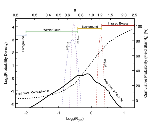
Figure 12: Probability distribution functions for the A_V ratio function $R_{2}$ ($\equiv$ A${}_{V_{O}}$ / A${}_{V_{I}}$), similar to the plot shown as Figure 6. The solid black curve displays the $R_{2}$ probability density for the background objects in the two observed fields. The dashed black curve is the corresponding cumulative $R_{2}$ probability. Dashed colored curves display the $R_{2}$ probability densities for the ITG objects 16, 19, and 21. Based on these curves, and the Gaia EDR3 distance to ITG 16, all three are judged to be more distant than HCl2.

Appendix B Lack of Time-Dependent EPA_O Changes

An alternative origin for the generation of net NIR polarizations for BD/YSO disk systems could involve shadowing due to warped inner disks causing anisotropic disk illumination (e.g., Benisty et al., 2018). A potential test of the application of this scenario to the objects in this study would be detection of time-dependent polarization properties. Indeed, both ITG 17 (at 2.95 days) and 2M0444 (at 4.43 days) exhibit periodic optical brightness amplitude variations, as detected using K2 (Howell et al., 2014) by Rebull et al. (2020), who attributed these to rotation.

The NIR polarization data obtained here for the six CFHT Tau 4 field observations (over 3 epochs) and the four 2M0444 field observations (2 epochs) were examined to test for significant polarization EPA_O variations. EPA_O deviations from the means, scaled by their uncertainties, were averaged to form a $\chi^{2}$ quantity for each of the objects in Table 1 plus three more comparison objects in the 2M0444 field. These comparison objects were chosen to have $H$-band brightnesses similar to that for 2M0444. All objects, except ITG 25, exhibited mean deviations in a narrow range of 0.8–1.2 $\sigma_{EPA_{O}}$ (i.e., reduced $\chi^{2}$ values of 0.6–1.5) with no evidence of higher deviation noise for ITG 15, ITG 17, or 2M0444 above the values shown by the other, non-disk ITG and comparison objects. ITG 25 showed a mean EPA_O deviation of 2.3 $\sigma_{EPA_{O}}$ (reduced $\chi^{2}$ of 5.3) but it also had the lowest $\sigma_{EPA_{O}}$ values of about 1.$\arcdeg$4, versus the 4–18$\arcdeg$ seen for the fainter objects. Although this study was not designed to probe the time-dependent behavior of the NIR polarization from BD or YSO disks, to the limits of these current observations, strong deviations in the polarization EPA_O values were not found.

Appendix C The Low-Polarization Object J04395: SED Comparisons

One star in the CFHT Tau 4 field, 2MASS J04395361+2557485 (hereafter J04395; number 10094 in Table 2), showed low polarization percentage ($P^{\prime}_{O}<1$%) and moderately high extinction (A${}_{V_{O}}\sim 9$ mag) based on its apparent $(H-M)$ color. The resulting polarization efficiency is nearly as low as the values seen for the ITG 15 YSO and ITG 17 BD, as noted in Section 3.5.1 and as seen in Figure 8. For the BD and YSO, their low PEs are the result of both intrinsic polarizations being modified by the HCl2 magnetic field polarization and the mid-infrared thermal emission contributions from the disks of the objects. Could J04395 also have a disk? Is J04395 also embedded in HCl2?

The apparent polarization properties of the object were corrected using the bulk Stokes correction method described in Section 3.5 and the results are listed in Table 6. The derived EPA_D of $82.9\pm 16.9$° for J04395 suggests that the disk polarization orientation may be perpendicular to the HCl2 magnetic field orientation. If it is embedded within HCl2, then this finding matches those for the other ITG objects. However, Gaia EDR3 lists no parallax or proper motion for this object, so its location remains unknown. No other objects in the CFHT Tau 4 or 2M0444 fields show PE values as low as seen for J04395.

Table 6: Stokes Parameters for J04395

Desig.	Quantities	Stokes $Q$	Stokes $U$	$P$	$\sigma_{P}$	$P^{\prime}$	EPA
		(%)	(%)	(%)	(%)	(%)	(°)
(1)	(2)	(3)	(4)	(5)	(6)	(7)	(8)
J04395	A: Observed ($X_{O}$)	$-$0.56$\pm$0.56	+0.70$\pm$0.57	0.90	0.56	0.69	64.5$\pm$23.3
	B: Interpolated ($X_{I}$)	$-$0.68$\pm$0.20	+1.86$\pm$0.20	1.98	0.20	1.97	55.1$\pm$2.8
	C: Residuals (Intrinsic) ($X_{R}$)	$+$0.12$\pm$0.59	$-$1.16$\pm$0.61	1.17	0.60	1.00	138.0$\pm$16.7
	D: Difference (= C - B) ($X_{D}$)						82.9$\pm$16.9

C.1 Spectral Energy Distributions

To try to understand the nature of J04395, SEDs for the BDs, the YSOs, the non-YSO ITG objects, and for J04395 were developed, using Vizier (Ochsenbein et al., 2000) to collect published spectral fluxes. The results are shown in Figure 13. The SEDs for the eight objects were grouped into two sets: those showing strong disk emission in mid-infrared (MIR) through mm wavelengths (ITG 15, ITG 17, ITG 25, and 2M0444) and those with weak or questionable MIR emission (ITG 16, ITG 19, ITG 21, and J04395). In Figure 13, the SEDs showing disk emission are colored different shades of red, while those lacking strong disk emission are colored different shades of blue. The SEDs were ordered by the strength of the disk MIR emission relative to the peak photospheric emission, from the strongest (ITG 25) to the weakest (ITG 16). Offsets were applied to each SED to reduce overlaps in the MIR range. The offsets were multiplicative and are listed as the base-10 log power in parentheses after the identifier for each object in the inset legend in the Figure. The SEDs have not been corrected for extinction effects.

The SED for J04395 is generically very similar to the other three in its diskless or weak-disk set of SEDs. There is some hint of an upturn at 22 $\mu$m in the WISE W4 band, which might imply a colder disk or envelope component, but the signal-to-noise is less than two, so evidence for any disk is weak. Longer wavelength data are not available and the star is relatively faint, so confidently resolving whether a disk is present will require some effort.

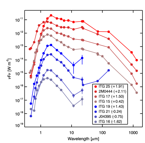
Figure 13: Spectral energy distributions (SEDs) of the two BDs, two YSOs, three non-YSO ITG stars, and the low-polarization star J04395. The upper four SEDs for the BDs and YSOs are colored in red shades and are ranked and offset to highlight long wavelength disk emission. The lower four SEDs for the non-YSOs are colored in blue shades and are similarly ranked and offset, as described in the text. The legend lists the objects and the base-10 power used to scale each SED.

The lack of strong disk emission in the MIR means that the observed $(H-M)$ reddening is fully due to dust extinction through HCl2. The A_V map for the CFHT Tau 4 field of Figure 4 predicts a total A${}_{V_{I}}$ through HCl2 at the position of J04395 of 9.8 mag, which gives a ratio $R_{2}$ of observed to interpolated A_V of 0.90. This falls in the ‘Background’ region designation shown in Figure 6. Thus, J04395 does not appear to be embedded within HCl2 and instead is behind the cloud. Hence, J04395 is not an embedded YSO or BD within the cloud and does not appear to exhibit emission from a strong disk or dusty envelope.

The question that remains is why the observed NIR polarization fraction for J04395 is so low, given the much higher values displayed by objects projected to be nearby on the sky and with similar apparent extinctions.

References

- Akeson et al. (2019) Akeson, R. L., Jensen, E. L. N., Carpenter, J., et al. 2019, ApJ, 872, 158. doi:10.3847/1538-4357/aaff6a
- Andersson et al. (2015) Andersson, B.-G., Lazarian, A., & Vaillancourt, J. E. 2015, ARA&A, 53, 501
- Andrews et al. (2013) Andrews, S. M., Rosenfeld, K. A., Kraus, A. L., et al. 2013, ApJ, 771, 129. doi:10.1088/0004-637X/771/2/129
- Andrews (2020) Andrews, S. M. 2020, ARA&A, 58, 483. doi:10.1146/annurev-astro-031220-010302
- Apai et al. (2004) Apai, D., Pascucci, I., Brandner, W., et al. 2004, A&A, 415, 671. doi:10.1051/0004-6361:20034549
- Arce et al. (1998) Arce, H. G., Goodman, A. A., Bastien, P., et al. 1998, ApJ, 499, L93. doi:10.1086/311337
- Asensio-Torres et al. (2016) Asensio-Torres, R., Janson, M., Hashimoto, J., et al. 2016, A&A, 593, A73. doi:10.1051/0004-6361/201628543
- Avenhaus et al. (2014) Avenhaus, H., Quanz, S. P., Schmid, H. M., et al. 2014, ApJ, 781, 87. doi:10.1088/0004-637X/781/2/87
- Ballering & Eisner (2019) Ballering, N. P. & Eisner, J. A. 2019, AJ, 157, 144. doi:10.3847/1538-3881/ab0a56
- Beckwith et al. (1990) Beckwith, S. V. W., Sargent, A. I., Chini, R. S., et al. 1990, AJ, 99, 924. doi:10.1086/115385
- Benisty et al. (2015) Benisty, M., Juhasz, A., Boccaletti, A., et al. 2015, A&A, 578, L6. doi:10.1051/0004-6361/201526011
- Benisty et al. (2018) Benisty, M., Juhász, A., Facchini, S., et al. 2018, A&A, 619, A171. doi:10.1051/0004-6361/201833913
- Benson & Myers (1989) Benson, P. J. & Myers, P. C. 1989, ApJS, 71, 89. doi:10.1086/191365
- Bouy et al. (2008) Bouy, H., Huélamo, N., Pinte, C., et al. 2008, A&A, 486, 877. doi:10.1051/0004-6361:20078866
- Brandt & Draine (2012) Brandt, T. D. & Draine, B. T. 2012, ApJ, 744, 129. doi:10.1088/0004-637X/744/2/129
- Bulger et al. (2014) Bulger, J., Patience, J., Ward-Duong, K., et al. 2014, A&A, 570, A29. doi:10.1051/0004-6361/201323088
- Chapman et al. (2011) Chapman, N. L., Goldsmith, P. F., Pineda, J. L., et al. 2011, ApJ, 741, 21. doi:10.1088/0004-637X/741/1/21
- Chen et al. (1995) Chen, H., Myers, P. C., Ladd, E. F., et al. 1995, ApJ, 445, 377. doi:10.1086/175703
- Clemens et al. (2020) Clemens, D. P., Cashman, L. R., Cerny, C., et al. 2020, ApJS, 249, 23. doi:10.3847/1538-4365/ab9f30
- Clemens et al. (2012c) Clemens, D. P., Pavel, M. D., & Cashman, L. R. 2012c, ApJS, 200, 21. doi:10.1088/0067-0049/200/2/21
- Clemens et al. (2012b) Clemens, D. P., Pinnick, A. P., & Pavel, M. D. 2012b, ApJS, 200, 20. doi:10.1088/0067-0049/200/2/20
- Clemens et al. (2012a) Clemens, D. P., Pinnick, A. P., Pavel, M. D., & Taylor, B. W. 2012a, ApJS, 200, 19. doi:10.1088/0067-0049/200/2/19
- Clemens et al. (2007) Clemens, D. P., Sarcia, D., Grabau, A., et al. 2007, PASP, 119, 1385. doi:10.1086/524775
- Clemens et al. (2016) Clemens, D. P., Tassis, K., & Goldsmith, P. F. 2016, ApJ, 833, 176. doi:10.3847/1538-4357/833/2/176
- Clemens et al. (2018) Clemens, D. P., El-Batal, A. M., Cerny, C., et al. 2018, ApJ, 867, 79. doi:10.3847/1538-4357/aae2af
- Cook et al. (2019) Cook, B. T., Tobin, J. J., Skrutskie, M. F., et al. 2019, A&A, 626, A51. doi:10.1051/0004-6361/201935419
- Davis & Greenstein (1951) Davis, L. & Greenstein, J. L. 1951, ApJ, 114, 206. doi:10.1086/145464
- Dobashi et al. (2005) Dobashi, K., Uehara, H., Kandori, R., et al. 2005, PASJ, 57, S1. doi:10.1093/pasj/57.sp1.S1
- Doi et al. (2020) Doi, Y., Hasegawa, T., Furuya, R. S., et al. 2020, ApJ, 899, 28. doi:10.3847/1538-4357/aba1e2
- Elias (1978) Elias, J. H. 1978, ApJ, 224, 857. doi:10.1086/156436
- Esposito et al. (2018) Esposito, T. M., Duchêne, G., Kalas, P., et al. 2018, AJ, 156, 47. doi:10.3847/1538-3881/aacbc9
- Esposito et al. (2020) Esposito, T. M., Kalas, P., Fitzgerald, M. P., et al. 2020, AJ, 160, 24. doi:10.3847/1538-3881/ab9199
- Follette et al. (2013) Follette, K. B., Tamura, M., Hashimoto, J., et al. 2013, ApJ, 767, 10. doi:10.1088/0004-637X/767/1/10
- Gaia Collaboration et al. (2016) Gaia Collaboration, Prusti, T., de Bruijne, J. H. J., et al. 2016, A&A, 595, A1 (Gaia). doi:10.1051/0004-6361/201629272
- Gaia Collaboration et al. (2018) Gaia Collaboration, Brown, A. G. A., Vallenari, A., et al. 2018, A&A, 616, A1 (Gaia DR2). doi:10.1051/0004-6361/201833051
- Gaia Collaboration et al. (2020) Gaia Collaboration, Brown, A. G. A., Vallenari, A., et al. 2020, arXiv:2012.01533 (Gaia EDR3)
- Galametz et al. (2018) Galametz, M., Maury, A., Girart, J. M., et al. 2018, A&A, 616, A139. doi:10.1051/0004-6361/201833004
- Galametz et al. (2020) Galametz, M., Maury, A., Girart, J. M., et al. 2020, A&A, 644, A47. doi:10.1051/0004-6361/202038854
- Galli et al. (2019) Galli, P. A. B., Loinard, L., Bouy, H., et al. 2019, A&A, 630, A137. doi:10.1051/0004-6361/201935928
- Garufi et al. (2018) Garufi, A., Benisty, M., Pinilla, P., et al. 2018, A&A, 620, A94. doi:10.1051/0004-6361/201833872
- Goodman et al. (1995) Goodman, A. A., Jones, T. J., Lada, E. A., et al. 1995, ApJ, 448, 748. doi:10.1086/176003
- Gray et al. (2018) Gray, W. J., McKee, C. F., & Klein, R. I. 2018, MNRAS, 473, 2124. doi:10.1093/mnras/stx2406
- Hales et al. (2006) Hales, A. S., Gledhill, T. M., Barlow, M. J., et al. 2006, MNRAS, 365, 1348. doi:10.1111/j.1365-2966.2005.09820.x
- Hall (1949) Hall, J. S. 1949, Science, 109, 166. doi:10.1126/science.109.2825.166
- Hiltner (1949a) Hiltner, W. A. 1949a, ApJ, 109, 471. doi:10.1086/145151
- Hiltner (1949b) Hiltner, W. A. 1949b, Science, 109, 165. doi:10.1126/science.109.2825.165
- Howell et al. (2014) Howell, S. B., Sobeck, C., Haas, M., et al. 2014, PASP, 126, 398
- Itoh et al. (1996) Itoh, Y., Tamura, M., & Gatley, I. 1996, ApJ, 465, L129 (ITG). doi:10.1086/310154
- Itoh et al. (1999) Itoh, Y., Tamura, M., & Nakajima, T. 1999, AJ, 117, 1471. doi:10.1086/300782
- Joncour et al. (2017) Joncour, I., Duchêne, G., & Moraux, E. 2017, A&A, 599, A14. doi:10.1051/0004-6361/201629398
- Joncour et al. (2018) Joncour, I., Duchêne, G., Moraux, E., et al. 2018, A&A, 620, A27. doi:10.1051/0004-6361/201833042
- Joye & Mandel (2003) Joye, W. A. & Mandel, E. 2003, Astronomical Data Analysis Software and Systems XII, 295, 489
- Kenyon et al. (1990) Kenyon, S. J., Hartmann, L. W., Strom, K. M., et al. 1990, AJ, 99, 869. doi:10.1086/115380
- Kristensen et al. (2012) Kristensen, L. E., van Dishoeck, E. F., Bergin, E. A., et al. 2012, A&A, 542, A8. doi:10.1051/0004-6361/201118146
- Lada et al. (1994) Lada, C. J., Lada, E. A., Clemens, D. P., & Bally, J. 1994, ApJ, 429, 694. doi:10.1086/174354
- Law et al. (2010) Law, N. M., Dhital, S., Kraus, A., et al. 2010, ApJ, 720, 1727. doi:10.1088/0004-637X/720/2/1727
- Lawrence et al. (2007) Lawrence, A., Warren, S. J., Almaini, O., et al. 2007, MNRAS, 379, 1599. doi:10.1111/j.1365-2966.2007.12040.x
- Lazarian & Hoang (2007) Lazarian, A. & Hoang, T. 2007, MNRAS, 378, 910. doi:10.1111/j.1365-2966.2007.11817.x
- Lodieu et al. (2009) Lodieu, N., Burningham, B., Hambly, N. C., et al. 2009, MNRAS, 397, 258. doi:10.1111/j.1365-2966.2008.14384.x
- Lombardi et al. (2010) Lombardi, M., Lada, C. J., & Alves, J. 2010, A&A, 512, A67. doi:10.1051/0004-6361/200912670
- Luhman (2012) Luhman, K. L. 2012, ARA&A, 50, 65. doi:10.1146/annurev-astro-081811-125528
- Luhman (2018) Luhman, K. L. 2018, AJ, 156, 271. doi:10.3847/1538-3881/aae831
- Luhman et al. (2010) Luhman, K. L., Allen, P. R., Espaillat, C., et al. 2010, ApJS, 186, 111. doi:10.1088/0067-0049/186/1/111
- Majewski et al. (2011) Majewski, S. R., Zasowski, G., & Nidever, D. L. 2011, ApJ, 739, 25. doi:10.1088/0004-637X/739/1/25
- Mathis et al. (1983) Mathis, J. S., Mezger, P. G., & Panagia, N. 1983, A&A, 500, 259
- Maury et al. (2019) Maury, A. J., André, P., Testi, L., et al. 2019, A&A, 621, A76. doi:10.1051/0004-6361/201833537
- Motte & André (2001) Motte, F. & André, P. 2001, A&A, 365, 440. doi:10.1051/0004-6361:20000072
- Narayanan et al. (2008) Narayanan, G., Heyer, M. H., Brunt, C., et al. 2008, ApJS, 177, 341. doi:10.1086/587786
- Ochsenbein et al. (2000) Ochsenbein, F., Bauer, P., & Marcout, J. 2000, A&AS, 143, 23. doi:10.1051/aas:2000169
- Pattle et al. (2019) Pattle, K., Lai, S.-P., Hasegawa, T., et al. 2019, ApJ, 880, 27. doi:10.3847/1538-4357/ab286f
- Pavel (2014) Pavel, M. D. 2014, AJ, 148, 49. doi:10.1088/0004-6256/148/3/49
- Pineda et al. (2010) Pineda, J. L., Goldsmith, P. F., Chapman, N., et al. 2010, ApJ, 721, 686. doi:10.1088/0004-637X/721/1/686
- Potter (2005) Potter, D. E. 2005, Astronomical Polarimetry: Current Status and Future Directions, 343, 143
- Rebull et al. (2020) Rebull, L. M., Stauffer, J. R., Cody, A. M., et al. 2020, AJ, 159, 273
- Ricci et al. (2013) Ricci, L., Isella, A., Carpenter, J. M., et al. 2013, ApJ, 764, L27. doi:10.1088/2041-8205/764/2/L27
- Ricci et al. (2014) Ricci, L., Testi, L., Natta, A., et al. 2014, ApJ, 791, 20. doi:10.1088/0004-637X/791/1/20
- Rilinger et al. (2019) Rilinger, A. M., Espaillat, C. C., & Macías, E. 2019, ApJ, 878, 103. doi:10.3847/1538-4357/ab211d
- Rosen et al. (2019) Rosen, A. L., Li, P. S., Zhang, Q., et al. 2019, ApJ, 887, 108. doi:10.3847/1538-4357/ab54c6
- Serkowski et al. (1975) Serkowski, K., Mathewson, D. S., & Ford, V. L. 1975, ApJ, 196, 261. doi:10.1086/153410
- Silber et al. (2000) Silber, J., Gledhill, T., Duchêne, G., et al. 2000, ApJ, 536, L89. doi:10.1086/312731
- Skrutskie et al. (2006) Skrutskie, M.F., Cutri, R. M., Stiening, R., et al. 2006, AJ, 131, 1163. doi:10.1086/498708
- Tamura & Sato (1989) Tamura, M. & Sato, S. 1989, AJ, 98, 1368. doi:10.1086/115222
- Taylor (2005) Taylor, M. B. 2005, Astronomical Data Analysis Software and Systems XIV, 347, 29
- Tobin et al. (2008) Tobin, J. J., Hartmann, L., Calvet, N., et al. 2008, ApJ, 679, 1364. doi:10.1086/587683
- Ward-Duong et al. (2018) Ward-Duong, K., Patience, J., Bulger, J., et al. 2018, AJ, 155, 54. doi:10.3847/1538-3881/aaa128
- Wright et al. (2010) Wright, E. L., Eisenhardt, P. R. M., Mainzer, A. K., et al. 2010, AJ, 140, 1868. doi:10.1088/0004-6256/140/6/1868
- Wurster & Bate (2019) Wurster, J. & Bate, M. R. 2019, MNRAS, 486, 2587. doi:10.1093/mnras/stz1023
- Yen et al. (2021) Yen, H.-W., Zhao, B., Koch, P. M., et al. 2021, ApJ, 916, 97. doi:10.3847/1538-4357/ac0723
- Zhao et al. (2018) Zhao, B., Caselli, P., Li, Z.-Y., et al. 2018, MNRAS, 473, 4868. doi:10.1093/mnras/stx2617
- Zhao et al. (2020) Zhao, B., Tomida, K., Hennebelle, P., et al. 2020, Space Sci. Rev., 216, 43. doi:10.1007/s11214-020-00664-z
- Zhang et al. (2018) Zhang, Z., Liu, M. C., Best, W. M. J., et al. 2018, ApJ, 858, 41. doi:10.3847/1538-4357/aab269