Quantum phases of ferromagnetically coupled dimers on Shastry-Sutherland lattice

Abstract

The ground state (gs) of antiferromagnetically coupled dimers on the Shastry-Sutherland lattice (SSL) stabilizes many exotic phases and has been extensively studied. The gs properties of ferromagnetically coupled dimers on SSL are equally important but unexplored. In this model the exchange coupling along the $x$-axis ($J_{x}$) and $y$-axis ($J_{y}$) are ferromagnetic and the diagonal exchange coupling ($J$) is antiferromagnetic. In this work we explore the quantum phase diagram of ferromagnetically coupled dimer model numerically using density matrix renormalization group (DMRG) method. We note that in $J_{x}$-$J_{y}$ parameter space this model exhibits six interesting phases:(I) stripe $(0,\pi)$, (II) stripe $(\pi,0)$, (III) perfect dimer, (IV) $X$-spiral, (V) $Y$-spiral and (VI) ferromagnetic phase. Phase boundaries of these quantum phases are determined using the correlation functions and gs energies. We also notice the correlation length in this system is less than four lattice units in most of the parameter regimes. The non-collinear behaviour in $X$-spiral and $Y$-spiral phase and the dependence of pitch angles on model parameters are also studied.

I Introduction

Frustrated magnetic systems are promising materials to explore exotic phases like dimer White et al. (1994), non-collinear spin wave Kumar et al. (2015), spin-liquid Zhou et al. (2017); Savary and Balents (2016), non-trivial topological phase Balents (2010); Lee (2008); Han et al. (2012); Fu et al. (2015) in the ground state (gs). In the last couple of decades these systems are extensively synthesized in various dimensions for example, in one dimensional geometry: LiCuSbO₄ Dutton et al. (2012), LiCuVO₄ Mourigal et al. (2012) and Rb₂Cu₂Mo₃O₁₂ Hase et al. (2004); Yagi et al. (2017); in ladder like geometry: SrCu₂O₃ Sandvik et al. (1996) and (VO)₂P₂O₇ Johnston et al. (1987); Dagotto and Rice (1996); in two dimensional systems such as ZnCu₃(OH)₆Cl₂(Herbertsmithite) Shores et al. (2005); Helton et al. (2007); Han et al. (2012) and $\alpha$-RuCl₃ Banerjee et al. (2016). Their properties have been rigorously explored theoretically as well Broholm et al. (2020); Lake et al. (2005); Norman (2016); Takagi et al. (2019). In presence of a finite magnetic field, these systems exhibit plethora of quantum phases like multipolar Fouet et al. (2006), spin nematic Shannon et al. (2006), vector chiral Hikihara et al. (2008), plateaus state at various fractional magnetization Leonov and Mostovoy (2015); Lee (2008); Balents (2010); Momoi and Totsuka (2000); Schulenburg et al. (2002). To explain the physical properties of these systems various models have been proposed like Heisenberg spin-1/2 $J_{1}$-$J_{2}$ model for one dimensional (1D) spin chain Majumdar and Ghosh (1969); White et al. (1994); Chitra et al. (1995); Soos et al. (2016), Heisenberg anti-ferromagnetic spin-1/2 model on Shastry-Sutherland lattice (SSL) Shastry and Sutherland (1981) and square lattice Chakravarty et al. (1989) , $J_{1}$-$J_{2}$ model on square lattice Dagotto and Moreo (1989); Sirker et al. (2006) etc.

In general, frustrated 2D magnets are found in layered materials Kundu et al. (2020) and these 2D geometries: square Manousakis (1991), triangular Shirata et al. (2012), kagome Helton et al. (2007) and SSL Kageyama et al. (1999); Zayed et al. (2017); Lee et al. (2019) are particularly interesting because 2D is supposed to be a critical dimension in the purview of Mermin-Wagner theorem Mermin and Wagner (1966). We are particularly interested in SSL which is shown in Fig. 1. This structure is similar to a square lattice except alternate squares have a diagonal bond. If a isotropic Heisenberg spin-1/2 model on the SSL is considered with antiferromagnetic exchange along the square $J_{x}=J_{y}$ and diagonal exchange $J=2J_{x}=2J_{y}$ then the model can be solved exactly Shastry and Sutherland (1981). The ground state of this system has Néel and dimer order for small and large $J/J_{y}$ limit respectively considering ($J_{x}=J_{y}$). Corboz et al. Corboz and Mila (2013) predicted the existence of a plaquette phase between Néel and dimer region using the PEPS technique, whereas, very recently, Yang et al.Yang et al. (2021) predicted a spin liquid phase. While it’s exact nature has been controversial, Ronquillo and Peterson Ronquillo and Peterson (2014) predicted the topological gs.

Among the layered magnetic materials, spin-1/2 layered copper oxyhalides (CuX)A_n-1B_nO_3n+1 are frustrated 2D magnets which have many interesting features just by tuning the composition . The CuX layers are sandwiched by non-magnetic layers, the anion orbitals are involved in exchange pathways but the cation orbitals replacement keeps the magnetic layer homogeneous. However, a small change in exchange interaction can be tuned by changing the lattice parameters, electrostatic fields, and crystal-field splittings Tsirlin et al. (2012). The tuning of anion and cation composition can drive the system across the quantum critical points. Experimental results suggest that the gs can be tuned to have a collective singlet with a spin gap in (CuCl)LaNb₂O₇, Kageyama et al. (2005a, b); Kitada et al. (2007); Yoshida et al. (2007), a collinear stripe magnetic order in (CuBr)LaNb₂O₇, Oba et al. (2006) and a magnetization plateau at 1/3 of the saturated moment in (CuBr)Sr₂Nb₃0₁₀ Tsujimoto et al. (2007).

(CuCl)LaNb₂O₇ was initially predicted as $S=1/2$ frustrated square lattice Kageyama et al. (2005a), however, band structure calculations revealed that the simplest model for this material can be best described as strong antiferromagnetic (AFM) exchange interaction between fourth neighbours forming a strong singlet dimer and these dimers are coupled together by ferromagnetic (FM) interactions i.e this model looks like the Shastry-Sutherland model with ferromagnetic exchange $J_{x}$ and $J_{y}$ along square and antiferromagnetic diagonal exchange $J$ Tassel et al. (2010). This model was theoretically studied using mean-field and exact diagonalization (ED) methods on a small cluster and they predicated a plethora of phases in exchange parameter space Furukawa et al. (2011). In the intermediate FM coupling limit, they reported two types of stripe phases, $(0,\pi)$ and $(\pi,0)$, separated by a non-collinear spiral phase. The dimer singlet stabilizes for $J_{x},J_{y}<J/2$, whereas ferromagnetic gs is stable for large $J_{x}$ and $J_{y}$ Furukawa et al. (2011). We notice that the phase boundaries as well as the existence of different phases calculated from ED are not consistent with that calculated from mean-field, for example, non-collinear phase does not appear in exact diagonalization results, but is present in the mean field calculations. Therefore, it is very intriguing to explore such an interesting model with a more sophisticated numerical tool like density matrix renormalization group (DMRG) method which can give accurate results for large lattice sizes.

In this work, we explore the ferromagnetically coupled $S=1/2$ dimers on SSL with the DMRG method and re-investigate the quantum phase diagram of this model. The phase diagram is based on the nature of spin-spin correlations and ground state energy variation. The gs exhibits predominantly six types of phases: two types of stripe order with wave vector $(0,\pi)$ and $(\pi,0)$ for large value $J_{y}$ and $J_{x}$ respectively. A perfect dimer phase exists for $J_{x}=J_{y}$ and this phase separates two types of spiral phases namely $X$-spiral with wave vector $(\theta,0)$ and $Y$-spiral with wavevector $(0,\theta)$, where $\theta$ is the pitch angle. In the large limit of $J_{x}$ and $J_{y}$ the gs has ferromagnetic behaviour. We also explore the effect of $J_{x}$ and $J_{y}$ on spiral behaviour and pitch angle and we notice that spin ordering is very short range in most of the parameter regimes.

The paper is organized as follows. In Sec. II , the model of the ferromagnetically coupled SSL and numerical methods are discussed. In Sec. III, all the numerical results are presented and this section has four subsections. The quantum phase diagram is presented in Sec. III.1. Sec. III.2 and Sec. III.3 discuss gs energy and spin-spin correlation in various phases of the phase diagram. The pitch angles are discussed in Sec. III.4. Results are discussed and compared with literature in Sec. IV. In an appendix we presented results for the ground state energy per site and spin-spin correlation for various bond dimensions ($m$) and various system sizes.

II Model Hamiltonian and numerical methods

We consider a Heisenberg spin $S=1/2$ model on SSL where only diagonal interaction $J=1$ is antiferromagnet and sets the energy scale of the system. The strength of ferromagnetic exchange interaction along the $x$-axis and $y$-axis on the square is represented by $J_{x}$ and $J_{y}$ respectively. The arrangement of the exchange interactions are shown in Fig. 1. Now onward we will call this model as Shastry-Sutherland (SSM) and can be written as

$$H=-J_{x}\sum_{<ij>_{x}}\vec{S}_{i}\cdot\vec{S}_{j}-J_{y}\sum_{<ij>_{y}}\vec{S}_{i}\cdot\vec{S}_{j}+J\sum_{<ij>_{d}}\vec{S}_{i}\cdot\vec{S}_{j}$$ (1)

where the first sum runs for NN bonds along the $x$-direction, the second sum runs for NN bonds along the $y$-direction and the last sum runs for NN diagonal bonds in the square.

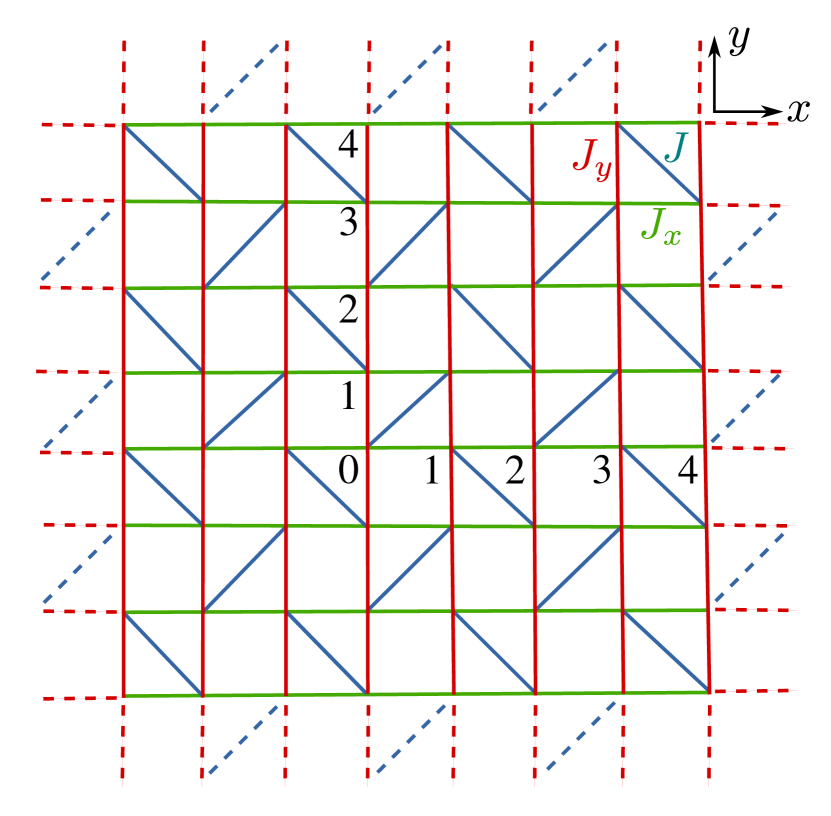
Figure 1: Figure shows a schematic diagram of SSL. The coupling constants along $x$-axis ($J_{x}$) and along $y$-axis ($J_{y}$) are FM and the diagonal bond couplings $J$ are AFM in nature. The site index $0$ is the reference site and the numbers along $x$-axis and $y$-axis represent the distance ($r$) from the reference site.

We use the exact diagonalization for system size up to 32 sites and the density matrix renormalization group (DMRG) method  White (1992, 1993); Schollwöck (2005); Hallberg (2006) for large system size. The DMRG method is a state of art numerical method to handle the large degrees of freedom for a many-body Hamiltonian in low dimensions. This method is based on the systematic truncation of irrelevant degrees of freedom while growing the system sizes and optimising the wavefunction while doing the finite DMRG algorithm. In this work, we use a modified DMRG method Kumar et al. (2010) in which 4-new sites are added at each step to reduce the number of times of renormalization of operators used to build the super block Kumar et al. (2010). We retain up to $m=900$ block states which are the eigenvectors of the system block density matrix corresponding to the largest eigenvalues. The chosen value of ‘$m$’ keeps the truncation error to less than $\sim 10^{-8}$. We also carry out $10-12$ finite sweeps for improved convergence and to optimise the wave function. We use cylindrical geometry of the SSL and a periodic boundary is applied along the width of the lattice and open boundary along the length. The largest system size studied is up to $12\times 8$ (length $\times$ width) system size. We have analysed the convergence of energy with the various values of $m$ in appendix. The per-site energies for $12\times 4$ system are shown for $m=256$, 512 and 900, whereas for $12\times 8$ system, it is shown for $m=256$, 512 and 700 in table 1. We notice that $m=512$ is sufficient for accuracy up to $5^{th}$ decimal place for $12\times 4$ and $4^{th}$ for $12\times 8$ system. We also show the dependence of the spin-spin correlation function on $m$ in table 2 and 3 of appendix. We notice that the spin-spin correlations are accurate up to $4^{th}$ decimal places. Interestingly this model gives amazing accuracy of energies as well as correlation function and these accuracy may be attributed to the short-range correlation length which is approximately $~{}4$ lattice unit.

III Results

To identify the existence of various phases of the model with isotropic Heisenberg exchange in Eq. 1, we calculate spin-spin correlation $C(r)$ and gs energies. There are six different phases in this model: (i) stripe $(0,\pi)$ where the spin configuration has a propagation vector $(k_{x},k_{y})=(0,\pi)$ and the system forms stripes along the $x$-direction where all the spins along $x$-direction are arranged ferromagnetically while spin modulates with wavevector $\pi$ along the $y$-direction as shown in Fig. 2(a). (ii) In the stripe $(\pi,0)$ phase, stripes run along the $y$-direction where spins are arranged ferromagnetically in $y$-direction while spin wave has wavevector $\pi$ along the $x$-direction as shown in Fig. 2(b). (iii) The ground state with a $X$-spiral phase has a non-collinear arrangement of spins along the $x$-direction and ferromagnetic ordering along the $y$-direction as shown in Fig. 2(c). This phase appears in case of highly frustrated model with AFM $J_{x}=J_{y}$ in Ref. [Shastry and Sutherland, 1981]. (iv) In $Y$-spiral phase, spins have a non-collinear arrangements along the $y$-direction and ferromagnetic ordering sets in along $x$-direction as in Fig. 2(d). (v) In the perfect dimer phase the gs wave function can be represented as a product of dimer singlets: $|\psi\rangle\equiv\prod_{d}~{}\frac{1}{\sqrt{2}}(|\uparrow\downarrow\rangle-|\downarrow\uparrow\rangle)_{d}$, where $d$ labels a dimer Shastry and Sutherland (1981); Furukawa et al. (2011). In this phase, the dimers are formed along the diagonal bonds as shown in Fig. 2 (e). The spin-spin correlation $C(r)=-0.75$ along the diagonal bonds and $C(r)=0$ along any other bonds on the square. (vi) When the FM couplings dominate over the diagonal antiferromagnetic exchange interaction the FM phase appears. In this phase, all spins are aligned in the same direction as shown in Fig. 2(f).

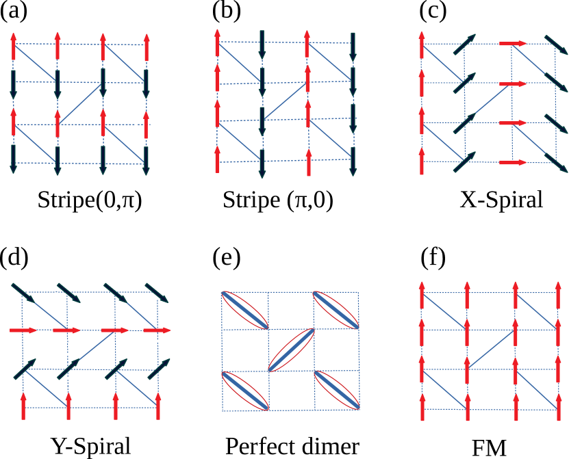
Figure 2: Figure shows a schematic diagram of different phases present in the ferromagnetically coupled dimers on the SSL, where arrows represent the spin alignments and the ellipses are the dimers (defined in the main text). (a) and (b) are two stripe phases with ordering wave vector $(0,\pi)$ and ($\pi,0$) respectively. (c) and (d) are two non-collinear spiral phases, the $X$-spiral and $Y$-spiral. (e) and (f) are the perfect dimer and FM phase respectively.

III.1 Quantum Phase Diagram

In this section, the quantum phase diagram is presented in $J_{x}$ and $J_{y}$ parameter space as shown in Fig.3 for a given diagonal exchange $J=1$. For a large value of $J_{x}$ or $J_{y}$ stripe phases with wave vectors $(0,\pi)$ and $(\pi,0)$ stabilized in the gs of the system. In this region, frustration is considerably small due to the small or large value of $J_{x}/J_{y}$. The strong FM coupling bonds prefer FM spin orderings, whereas, weak FM coupling bonds prefer antiferromagnetic spin ordering to satisfy the diagonal AFM exchange.

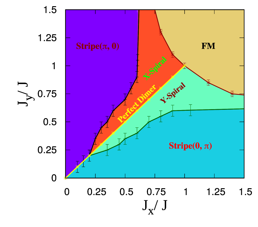
Figure 3: Figure shows the quantum phase diagram of the SSM. The phase diagram comprises six phases: Two stripe order phases with ordering wave vector $(0,\pi)$ and $(\pi,0)$, two spiral orders along both the $x$- and $y$-directions, the $X$-spiral and $Y$-spiral phase respectively. The other two phases are a perfect dimer phase (the yellow line separating two spiral phases) and a phase with FM spin ordering along all directions of the lattice.

For the moderate exchange strength $J_{x}<1$ and $J_{y}<1$ the gs has non-collinear spin ordering. Depending on the relative exchange strength of $J_{x}$ and $J_{y}$ there are two types of spiral phases: $X$-spiral and $Y$-spiral. These two spiral phases are separated by a perfect dimer phase formed along the line $J_{x}=J_{y}$ and extended up to $J_{x},J_{y}\lesssim J$. The perfect dimer region is confined along the $J_{x}=J_{y}$ line as $C(r=2)$ continuously increases with $|J_{x}-J_{y}|$. In the strong coupling region of $J_{x}$ and $J_{y}$, long-range FM magnetic ordering sets in.

III.2 Ground state energy

Ground state energies are calculated for the model in Eq. 1 on a cylindrical geometry with periodic boundary condition (PBC) along the width ($y$-axis) and open boundary condition along the length ($x$-axis), and $12\times 4$ system is used to calculate the accurate gs. In Fig. 4 the gs energy per site $\epsilon_{gs}$ is plotted as a function of $J_{y}$ by keeping $J_{x}$ fixed value of $J_{x}=0.9$. Around $J_{y}\sim 1.1$ we saw a discontinuity in the gs energy, indicating a first-order phase transition from FM to $X$-spiral phase. The maxima of the energy curve is close to $J_{x}=J_{y}\sim 0.9$ which indicates the dimer line, and the small deviation of maxima from dimer line $J_{x}=J_{y}$ is due to the rectangular geometry of the lattice. The maxima shifts to $J_{x}=J_{y}$ line as we increase the width of the lattice. The smooth variation of $\epsilon_{gs}$ with $J_{y}$ indicates the second-order dimer transition. No signature of spiral and stripe transitions is detected from the gs energy variation.

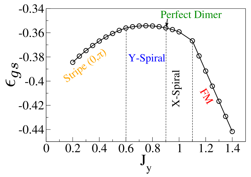
Figure 4: Figure shows gs energy per site ($\epsilon_{gs}$) versus $J_{y}$ plot at $J_{x}=0.9$ for $12\times 4$ lattice sites of the SSM. Around $J_{y}=1.1$ we show a kink in the energy curve indicating a sharp phase transition from $X$-spiral to FM phase. The transition between the two spiral phases is not sharp. Around $J_{y}=0.6$ system transits from $Y$-spiral to stripe $(0,\pi)$ phase. (Shaded lines are only for eye guide of the transition points).

III.3 Spin-spin correlation

In this subsection, we present spin-spin correlation $C(r)$ for various parameter regimes to validate the existence of different phases in the phase diagram in Fig. 3. We are dealing with isotropic system and total spin-spin correlations $C(r)=\langle\vec{S}_{i}\cdot\vec{S}_{i+r}\rangle=3\langle S^{z}_{i}S^{z}_{i+r}\rangle$ where $S^{z}_{i}$ represents the $z$-component of the spin operator at the reference site $i$. $r$ is the distance between the spin site and reference site along the $x$- and $y$-axis as shown in Fig. 1. The spin Hamiltonian in Eq. 1 has $SU(2)$ symmetry and one expects equal spin-spin correlation for all three spin components in the singlet sector. To understand the spin arrangements in different phases we have calculated $C(r)$ along different spatial directions. In Fig. 1, the site with $0$ index represents the reference site, from which correlations are calculated in various directions, and distances $r$ are shown in various directions with numerials as shown in Fig. 1.

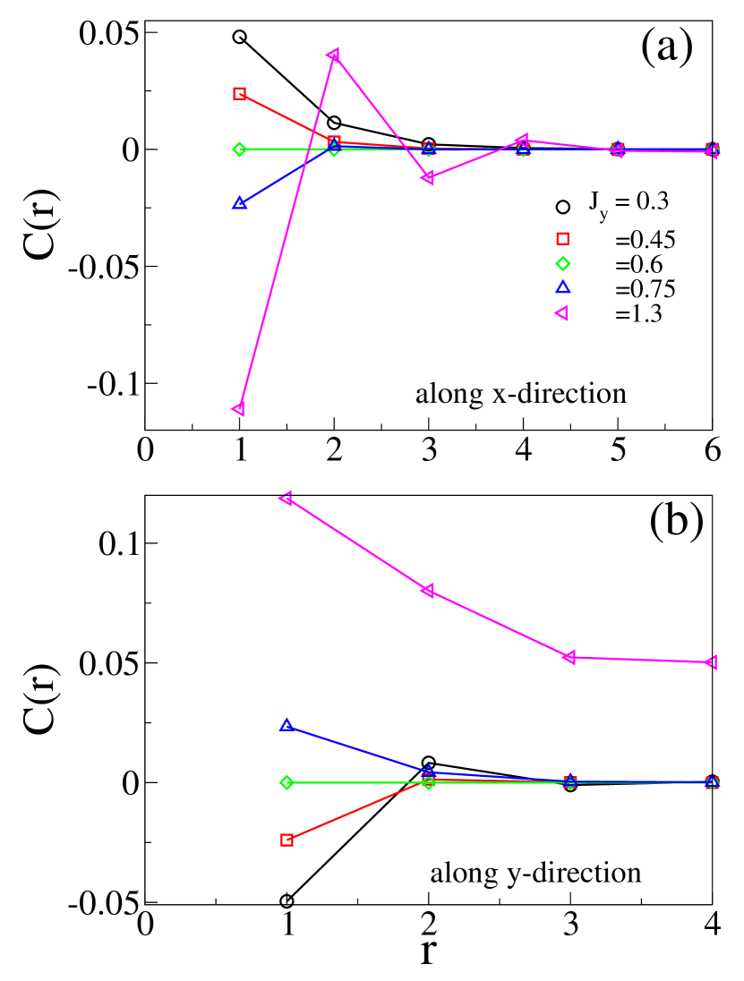
Figure 5: Figure shows the variation of spin-spin correlations $C(r)$ with distance $(r)$ for $12\times 8$ system size. Spin-spin correlations are calculated for different $J_{y}$ values by keeping $J_{x}$ fixed at $0.6$. (a) $C(r)$ are calculated along $x$-direction. (b) $C(r)$ are calculated along $y$-direction.

In Fig. 5(a) we presented $C(r)$ along the $x$-direction, whereas Fig. 5 (b) represents the same for $y$-direction. In all plots, we have fixed $J_{x}=0.6$ and calculated $C(r)$ for different $J_{y}=0.3$, 0.45, 0.6, 0.75 and 1.3, where $J_{y}$ values correspond to different phases in the phase diagram.

In Fig. 5(a) for $J_{y}=0.3$, all the values of $C(r)$ are positive which correspond to an FM spin arrangment along $x$-direction. Whereas in Fig. 5(b) for same value of $J_{y}=0.3$, $C(r)$ shows an antiferromagnetic arrangement of spins along $y$-direction. This kind of spin arrangements correspond to a stripe spin ordering with a wave vector $(0,\pi)$ (see Fig.2(a)). For $J_{y}=1.3$ the behaviour of the spin correlation along the $x$-direction interchanges with the behaviour along $y$-direction i.e antiferromagnetic arrangement along the $x$-direction and ferromagnetic arrangement along the $y$-direction. This represents another kind of stripe phase with wave vector at $(\pi,0)$ as shown in Fig. 2(b).

At $J_{y}=0.45$, $C(r)$ along $x$-direction are all positive and correspond to an FM spin alignment in this direction, whereas in the $y$-direction the $C(r)$ is non-collinear i.e pitch angle is different from 0 or $\pi$. The non-collinear spin arrangement is shown along the $y$-direction and the $Y$-spiral phase can be seen in Fig. 2(d). For $J_{y}=0.75$, $C(r)$ shows a non-collinear behaviour along $x$-direction whereas ferromagnetic behaviour along the $y$-direction. The schematic of $X$-spiral phase is shown in Fig. 2(c).

When $J_{x}=J_{y}(=0.6)$, $C(r)$ along $x$-direction and $y$-direction are exactly zero, whereas, we found the correlation for diagonal bonds are $-0.75$ This shows a perfect dimer formation along the diagonal bonds and this phase is shown in Fig. 2(e). A perfect dimer phase is formed along $J_{x}=J_{y}\lesssim 1$ line. In low $J_{x}$ and $J_{y}$ limit $C(r>1)$ have non zero value for $|J_{x}-J_{y}|>0$, therefore the perfect dimer phase is only restricted to $J_{x}=J_{y}$. In the FM phase region $C(r)$ have all positive values in all directions.

III.4 Pitch angle

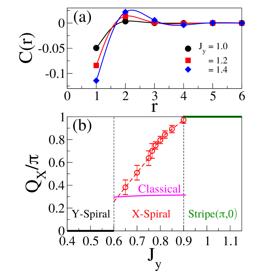
Figure 6: Figure (a) shows the spin-spin correlation $C(r)$ along length ($x$-direction) for different $J_{y}$ at $J_{x}=0.7$. The solid curves represent respective fits with exponential decaying function. In figure (b) we have plotted pitch angle $(Q_{x}/\pi)$ as a function of $J_{y}$ at $J_{x}=0.6$ for different phases of the model, where $Q_{x}$ is the pitch angle for the $X$-spiral phase varying along $x$-direction. The pink line is the value of pitch angles calculated using Eq. 3. In both plots we have used $12\times 4$ system size.

In a geometrically frustrated system wavevector or the pitch angle of a non-collinear spin ordering, in general, depends on the competing exchange interactions Furukawa et al. (2012); Parvej and Kumar (2017); Maiti and Kumar (2019) and therefore, it is important to understand behaviour of pitch angle $\theta$ in various exchange interaction limits to quantify spin modulation in terms of the pitch angle $Q_{x}$ and $Q_{y}$. Fig. 6(a) shows spin-spin correlation $C(r)$ for $J_{x}=0.7$ for different $J_{y}$ values inside the $X$-spiral region. $C(r)$ shows the exponentially decaying behaviour with distance r. It indicates the non-collinear spin ordering along $x$-direction, representing the $X$-spiral phase. $C(r)$ in Fig. 6(a) shows an exponential decay, representing a very short-range correlation in the spiral region. Pitch angle $(Q_{x})$ can be calculated in the $X$-spiral phase, by fitting $C(r)$ with the following equation

$$C(r)=a_{0}\cos(Q_{x}r+c)~{}e^{-\frac{r}{\xi}}~{},$$ (2)

where $\xi$ is the correlation length, $a_{0}$ and $c$ are constants. To calculate the pitch angles in the $Y$-spiral phase, a similar correlation function can be applied as above, where $Q_{x}$ will be replaced by $Q_{y}$. The variation of pitch angle $Q_{x}$ with $J_{y}$ is presented in Fig. 6(b) and we notice that $Q_{x}$ varies between $0$ to $\pi$. We also notice that $Q_{x}$ changes sharply near $J_{x}\sim 0.6$. $Q_{x}$ and $Q_{y}$ variation with $J_{y}$ and $J_{x}$ for a classical system Furukawa et al. (2011) can be given as

$$\cos(Q_{x}) = -\frac{J_{y}}{J}+\frac{J}{4J_{x}}\left(\frac{J_{y}}{J_{x}}-\frac{J_{x}}{J_{y}}\right),$$

$$\cos(Q_{y}) = -\frac{J_{x}}{J}+\frac{J}{4J_{y}}\left(\frac{J_{x}}{J_{y}}-\frac{J_{y}}{J_{x}}\right)~{}.$$ (3)

The classical results seem to deviate significantly from our calculated values. The DMRG results are shown as dotted line with circles whereas the classical results are shown as solid line as shown in Fig. 6(b). The calculated values of $Q_{x}$ suggest that it is zero below the dimer line and increase rapidly with $J_{y}$ and reaches to $\pi$ for $J_{y}\sim 1.0$. In the stripe $(\pi,0)$ phase the $Q_{x}$ is $\pi$, whereas it is zero in the stripe $(0,\pi)$ phase. These systems have correlation length $\xi\approx 4$ lattice units, therefore, there is an error in calculating the $Q_{x}$ and it is represented by error bars. The system remains invariant by exchanging the $J_{y}$ to $J_{x}$ interaction, therefore $Q_{x}-J_{y}$ and $Q_{y}-J_{x}$ curves have the same nature as shown in $Q_{x}-J_{y}$ curve.

IV Summary and conclusion

In this work, we construct a new quantum phase diagram of ferromagnetically coupled $S=1/2$ on the SSL. Exchange couplings along width $J_{y}$ and length $J_{x}$ are ferromagnetic, whereas, the exchange couplings along diagonal bonds $J$ are antiferromagnetic. The quantum phase diagram of the SSM in Eq. 1 consists of six phases and the phase boundaries are calculated based on spin-spin correlation and the gs energies obtained using the ED and the DMRG methods. Our numerical calculations are done upto $12\times 8$ lattices and we have used PBC along the width and OBC along length. Almost everywhere in the phase space the order is short range and correlation length $\xi$ is less than equal to $4$ lattice unit, therefore, most of our calculations give reliable results for the two dimensional lattice of this model. The six phases in the phase diagrams are: (I) stripe $(0,\pi)$, (II) stripe $(\pi,0)$, (III) perfect dimer, (IV) $X$-spiral, (V) $Y$-spiral and (VI) ferromagnetic state. Our analysis also confirms the existence of spiral phases in this model for moderate FM couplings strength.

Our DMRG results are very different from the Schwinger-Boson mean-field theory in Ref. [Furukawa et al., 2011]. Although quantum phases predicted by mean-field theory are also found in the DMRG results but phases boundaries are quite different. DMRG calculations suggest that perfect dimer singlet phase is confined to only on $J_{x}=J_{y}$ line, whereas the mean-field calculation suggests a large area of this regime. Our result is consistent with the ED results Furukawa et al. (2011). Our results also suggest that second nearest neighbour correlation increases continuously with $|J_{x}-J_{y}|$ i.e. short range but finite correlation exists in the neighbourhood of dimer line except the $J_{x}=J_{y}$ line where only diagonal correlations are non zero. The mean-field results suggest the non-collinear spin wave along the $x$- and $y$-direction but ED does not confirm the results Furukawa et al. (2011). DMRG results confirm both types of the non-collinear phases. The mean-field pitch angle variation is small compared to the DMRG value in most parts of the parameter regime.

Tassel et al. suggested that (CuCl)LaNb₂O₇ has ferromagnetic $J_{y}/J\sim 0.39$ and $J_{x}/J\sim 0.38$ Tassel et al. (2010) and therefore, we expect this system should behave like dimer as it is on $J_{x}=J_{y}$ dimer singlet line. Although, Tsirlin et al. shows different exchange interactions using the two types of DFT calculations Tsirlin et al. (2012). However, the data of inelastic neutron scattering (INS) on powder samples shows that the dynamical structure factor has $S(Q,\omega)$ maxima around $Q\sim 0.5$Å, i.e. it is in a non-collinear regime. In our opinion this material is in the neighbourhood of dimer phase but detailed theoretical investigation is required to understand the spin configuration in the system.

In conclusion, we numerically studied the SSM and constructed a new quantum phase diagram using the DMRG method. We have also calculated the correlation function and pitch angle which can be directly connected to INS data. The phase boundaries calculated from DMRG results are different from that of mean-field and ED calculations . We hope that interesting quantum phases in real material like (CuCl)LaNb₂O₇ and others Tassel et al. (2010); Uemura et al. (2009); Kitada et al. (2009); Tsujimoto et al. (2009) can be revisited in light of this study. The short-range spiral phase in the frustrated regime of the model can be manipulated by external probe like a magnetic field, doping, etc. and might lead to many interesting phases. The effect of field on phase diagram of the model in Eq. 1 is still an open problem.

V Appendix

$L_{x}\times L_{y}$	$J_{x}$	$J_{y}$	$m$	$\epsilon_{gs}$
$12\times 4$	0.6	0.21	256	-0.357791
			512	-0.357795
			900	-0.357798
$12\times 8$	0.6	1.0	256	-0.36989
			512	-0.36987
			700	-0.36984

Table 1: The table shows the gs energy per site ($\epsilon_{gs}$) calculated for various bond dimensions ($m$). For the system size $12\times 4$ gs energy calculated for $J_{x}=0.6$ and $J_{y}=0.21$, whereas for $12\times 8$ system size, it is calculated for $J_{x}=0.6$ and $J_{y}=1.0$.

direction	$r$	$m=256$	$m=512$	$m=900$
length	1	0.02154	0.02153	0.02152
	2	0.00652	0.00651	0.00650
	3	0.00182	0.00182	0.00178
	4	0.00056	0.00056	0.00053
	5	0.00015	0.00015	0.00014
width	1	-0.02269	-0.02269	-0.02267
	2	0.01006	0.01006	0.01008

Table 2: The table shows spin-spin correlation $\langle S^{z}_{i}S^{z}_{i+r}\rangle$ calculated for various bond dimensions ($m$) for $12\times 4$ system size. The correlation calculated along length and width for $J_{x}=0.6$ and $J_{y}=0.21$, where the last three columns are the correlation values for the corresponding $m$.

direction	$r$	$m=256$	$m=512$	$m=700$
length	1	-0.02095	-0.02097	-0.02088
	2	0.00354	0.00338	0.00328
	3	-0.00037	-0.00032	-0.00030
	4	0.000058	0.000050	0.000042
	5	-0.000006	-0.000019	-0.000004
	6	-0.000001	0.000033	0.000001
width	1	0.021093	0.021144	0.021042
	2	0.008490	0.008516	0.008512
	3	0.002574	0.002553	0.002526
	4	0.001771	0.001719	0.001769

Table 3: The table shows spin-spin correlation $\langle S^{z}_{i}S^{z}_{i+r}\rangle$ calculated for various bond dimensions ($m$) for $12\times 8$ system size. The correlation calculated along length and width for $J_{x}=0.6$ and $J_{y}=1.0$, where the last three columns are the correlation values for the corresponding $m$.

References

- White et al. (1994) S. White, R. Noack, and D. Scalapino, Physical Review Letters 73, 886 (1994).
- Kumar et al. (2015) M. Kumar, A. Parvej, and Z. G. Soos, Journal of Physics: Condensed Matter 27, 316001 (2015).
- Zhou et al. (2017) Y. Zhou, K. Kanoda, and T.-K. Ng, Reviews of Modern Physics 89, 025003 (2017).
- Savary and Balents (2016) L. Savary and L. Balents, Reports on Progress in Physics 80, 016502 (2016).
- Balents (2010) L. Balents, Nature 464, 199 (2010).
- Lee (2008) P. A. Lee, Science 321, 1306 (2008).
- Han et al. (2012) T.-H. Han, J. S. Helton, S. Chu, D. G. Nocera, J. A. Rodriguez-Rivera, C. Broholm, and Y. S. Lee, Nature 492, 406 (2012).
- Fu et al. (2015) M. Fu, T. Imai, T.-H. Han, and Y. S. Lee, Science 350, 655 (2015).
- Dutton et al. (2012) S. Dutton, M. Kumar, M. Mourigal, Z. G. Soos, J.-J. Wen, C. L. Broholm, N. H. Andersen, Q. Huang, M. Zbiri, R. Toft-Petersen, et al., Physical Review Letters 108, 187206 (2012).
- Mourigal et al. (2012) M. Mourigal, M. Enderle, B. Fåk, R. Kremer, J. Law, A. Schneidewind, A. Hiess, and A. Prokofiev, Physical Review Letters 109, 027203 (2012).
- Hase et al. (2004) M. Hase, H. Kuroe, K. Ozawa, O. Suzuki, H. Kitazawa, G. Kido, and T. Sekine, Physical Review B 70, 104426 (2004).
- Yagi et al. (2017) A. Yagi, K. Matsui, T. Goto, M. Hase, and T. Sasaki, in Journal of Physics: Conference Series, Vol. 828 (IOP Publishing, 2017) p. 012016.
- Sandvik et al. (1996) A. W. Sandvik, E. Dagotto, and D. J. Scalapino, Physical Review B 53, R2934 (1996).
- Johnston et al. (1987) D. Johnston, J. Johnson, D. Goshorn, and A. Jacobson, Physical Review B 35, 219 (1987).
- Dagotto and Rice (1996) E. Dagotto and T. Rice, Science 271, 618 (1996).
- Shores et al. (2005) M. P. Shores, E. A. Nytko, B. M. Bartlett, and D. G. Nocera, Journal of the American Chemical Society 127, 13462 (2005).
- Helton et al. (2007) J. Helton, K. Matan, M. Shores, E. Nytko, B. Bartlett, Y. Yoshida, Y. Takano, A. Suslov, Y. Qiu, J.-H. Chung, et al., Physical Review Letters 98, 107204 (2007).
- Banerjee et al. (2016) A. Banerjee, C. Bridges, J.-Q. Yan, A. Aczel, L. Li, M. Stone, G. Granroth, M. Lumsden, Y. Yiu, J. Knolle, et al., Nature Materials 15, 733 (2016).
- Broholm et al. (2020) C. Broholm, R. Cava, S. Kivelson, D. Nocera, M. Norman, and T. Senthil, Science 367 (2020).
- Lake et al. (2005) B. Lake, D. A. Tennant, C. D. Frost, and S. E. Nagler, Nature Materials 4, 329 (2005).
- Norman (2016) M. Norman, Reviews of Modern Physics 88, 041002 (2016).
- Takagi et al. (2019) H. Takagi, T. Takayama, G. Jackeli, G. Khaliullin, and S. E. Nagler, Nature Reviews Physics 1, 264 (2019).
- Fouet et al. (2006) J.-B. Fouet, F. Mila, D. Clarke, H. Youk, O. Tchernyshyov, P. Fendley, and R. Noack, Physical Review B 73, 214405 (2006).
- Shannon et al. (2006) N. Shannon, T. Momoi, and P. Sindzingre, Physical Review Letters 96, 027213 (2006).
- Hikihara et al. (2008) T. Hikihara, L. Kecke, T. Momoi, and A. Furusaki, Physical Review B 78, 144404 (2008).
- Leonov and Mostovoy (2015) A. Leonov and M. Mostovoy, Nature Communications 6, 1 (2015).
- Momoi and Totsuka (2000) T. Momoi and K. Totsuka, Physical Review B 62, 15067 (2000).
- Schulenburg et al. (2002) J. Schulenburg, A. Honecker, J. Schnack, J. Richter, and H.-J. Schmidt, Physical Review Letters 88, 167207 (2002).
- Majumdar and Ghosh (1969) C. K. Majumdar and D. K. Ghosh, Journal of Mathematical Physics 10, 1388 (1969).
- Chitra et al. (1995) R. Chitra, S. Pati, H. Krishnamurthy, D. Sen, and S. Ramasesha, Physical Review B 52, 6581 (1995).
- Soos et al. (2016) Z. G. Soos, A. Parvej, and M. Kumar, Journal of Physics: Condensed Matter 28, 175603 (2016).
- Shastry and Sutherland (1981) B. S. Shastry and B. Sutherland, Physica B+ C 108, 1069 (1981).
- Chakravarty et al. (1989) S. Chakravarty, B. I. Halperin, and D. R. Nelson, Physical Review B 39, 2344 (1989).
- Dagotto and Moreo (1989) E. Dagotto and A. Moreo, Physical Review Letters 63, 2148 (1989).
- Sirker et al. (2006) J. Sirker, Z. Weihong, O. Sushkov, and J. Oitmaa, Physical Review B 73, 184420 (2006).
- Kundu et al. (2020) S. Kundu, A. Shahee, A. Chakraborty, K. Ranjith, B. Koo, J. Sichelschmidt, M. T. Telling, P. Biswas, M. Baenitz, I. Dasgupta, et al., Physical Review Letters 125, 267202 (2020).
- Manousakis (1991) E. Manousakis, Reviews of Modern Physics 63, 1 (1991).
- Shirata et al. (2012) Y. Shirata, H. Tanaka, A. Matsuo, and K. Kindo, Physical Review Letters 108, 057205 (2012).
- Kageyama et al. (1999) H. Kageyama, K. Yoshimura, R. Stern, N. Mushnikov, K. Onizuka, M. Kato, K. Kosuge, C. Slichter, T. Goto, and Y. Ueda, Physical Review Letters 82, 3168 (1999).
- Zayed et al. (2017) M. Zayed, C. Rüegg, A. Läuchli, C. Panagopoulos, S. Saxena, M. Ellerby, D. McMorrow, T. Strässle, S. Klotz, G. Hamel, et al., Nature Physics 13, 962 (2017).
- Lee et al. (2019) J. Y. Lee, Y.-Z. You, S. Sachdev, and A. Vishwanath, Physical Review X 9, 041037 (2019).
- Mermin and Wagner (1966) N. D. Mermin and H. Wagner, Physical Review Letters 17, 1133 (1966).
- Corboz and Mila (2013) P. Corboz and F. Mila, Physical Review B 87, 115144 (2013).
- Yang et al. (2021) J. Yang, A. W. Sandvik, and L. Wang, arXiv preprint arXiv:2104.08887 (2021).
- Ronquillo and Peterson (2014) D. C. Ronquillo and M. R. Peterson, Physical Review B 90, 201108 (2014).
- Tsirlin et al. (2012) A. A. Tsirlin, A. M. Abakumov, C. Ritter, and H. Rosner, Physical Review B 86, 064440 (2012).
- Kageyama et al. (2005a) H. Kageyama, T. Kitano, N. Oba, M. Nishi, S. Nagai, K. Hirota, L. Viciu, W. JB, J. Yasuda, Y. Baba, et al., Journal of the Physical Society of Japan 74, 1702 (2005a).
- Kageyama et al. (2005b) H. Kageyama, J. Yasuda, T. Kitano, K. Totsuka, Y. Narumi, M. Hagiwara, K. Kindo, Y. Baba, N. Oba, Y. Ajiro, et al., Journal of the Physical Society of Japan 74, 3155 (2005b).
- Kitada et al. (2007) A. Kitada, Z. Hiroi, Y. Tsujimoto, T. Kitano, H. Kageyama, Y. Ajiro, and K. Yoshimura, Journal of the Physical Society of Japan 76, 093706 (2007).
- Yoshida et al. (2007) M. Yoshida, N. Ogata, M. Takigawa, J.-i. Yamaura, M. Ichihara, T. Kitano, H. Kageyama, Y. Ajiro, and K. Yoshimura, Journal of the Physical Society of Japan 76, 104703 (2007).
- Oba et al. (2006) N. Oba, H. Kageyama, T. Kitano, J. Yasuda, Y. Baba, M. Nishi, K. Hirota, Y. Narumi, M. Hagiwara, K. Kindo, et al., Journal of the Physical Society of Japan 75, 113601 (2006).
- Tsujimoto et al. (2007) Y. Tsujimoto, Y. Baba, N. Oba, H. Kageyama, T. Fukui, Y. Narumi, K. Kindo, T. Saito, M. Takano, Y. Ajiro, et al., Journal of the Physical Society of Japan 76, 063711 (2007).
- Tassel et al. (2010) C. Tassel, J. Kang, C. Lee, O. Hernandez, Y. Qiu, W. Paulus, E. Collet, B. Lake, T. Guidi, M.-H. Whangbo, et al., Physical Review Letters 105, 167205 (2010).
- Furukawa et al. (2011) S. Furukawa, T. Dodds, and Y. B. Kim, Physical Review B 84, 054432 (2011).
- White (1992) S. R. White, Physical Review Letters 69, 2863 (1992).
- White (1993) S. R. White, Physical Review B 48, 10345 (1993).
- Schollwöck (2005) U. Schollwöck, Reviews of Modern Physics 77, 259 (2005).
- Hallberg (2006) K. A. Hallberg, Advances in Physics 55, 477 (2006).
- Kumar et al. (2010) M. Kumar, Z. G. Soos, D. Sen, and S. Ramasesha, Physical Review B 81, 104406 (2010).
- Furukawa et al. (2012) S. Furukawa, M. Sato, S. Onoda, and A. Furusaki, Physical Review B 86, 094417 (2012).
- Parvej and Kumar (2017) A. Parvej and M. Kumar, Physical Review B 96, 054413 (2017).
- Maiti and Kumar (2019) D. Maiti and M. Kumar, Physical Review B 100, 245118 (2019).
- Uemura et al. (2009) Y. Uemura, A. Aczel, Y. Ajiro, J. Carlo, T. Goko, D. Goldfeld, A. Kitada, G. Luke, G. MacDougall, I. Mihailescu, et al., Physical Review B 80, 174408 (2009).
- Kitada et al. (2009) A. Kitada, Y. Tsujimoto, H. Kageyama, Y. Ajiro, M. Nishi, Y. Narumi, K. Kindo, M. Ichihara, Y. Ueda, Y. Uemura, et al., Physical Review B 80, 174409 (2009).
- Tsujimoto et al. (2009) Y. Tsujimoto, A. Kitada, H. Kageyama, M. Nishi, Y. Narumi, K. Kindo, Y. Kiuchi, Y. Ueda, Y. J. Uemura, Y. Ajiro, et al., Journal of the Physical Society of Japan 79, 014709 (2009).