Fast and Accurate End-to-End Span-based Semantic Role Labeling as Word-based Graph Parsing

Abstract

This paper proposes to cast end-to-end span-based SRL as a word-based graph parsing task. The major challenge is how to represent spans at the word level. Borrowing ideas from research on Chinese word segmentation and named entity recognition, we propose and compare four different schemata of graph representation, i.e., BES, BE, BIES, and BII, among which we find that the BES schema performs the best. We further gain interesting insights through detailed analysis. Moreover, we propose a simple constrained Viterbi procedure to ensure the legality of the output graph according to the constraints of the SRL structure. We conduct experiments on two widely used benchmark datasets, i.e., CoNLL05 and CoNLL12. Results show that our word-based graph parsing approach achieves consistently better performance than previous results, under all settings of end-to-end and predicate-given, without and with pre-trained language models (PLMs). More importantly, our model can parse 669/252 sentences per second, without and with PLMs respectively.

1 Introduction

As a fundamental natural language processing (NLP) task, semantic role labeling (SRL) uses predicate-argument structure to represent the shallow semantic meaning of sentences. SRL structure is shown to be helpful for many downstream NLP tasks, such as machine translation (Liu and Gildea, 2010; Marcheggiani et al., 2018) and question answering (Wang et al., 2015).

There exist two forms of concrete SRL formalism in the community, i.e., word-based (also known as dependency-based SRL) and span-based, depending on whether an argument consists of a single word or a word span. Compared with word-based SRL, span-based SRL is more complex due to difficulties in determining argument boundaries. Figure 1 shows the span-based SRL structure for two predicates. Semantic roles of arguments are distinguished with edge labels, such as “A0” (agent) and “A1” (patient). This work focuses on the end-to-end span-based SRL task, and proposes a unified model to simultaneously recognize predicates and arguments in the input sentence.

In recent years, span-based SRL has achieved substantial performance boost due to the tremendous progress made by deep neural network models, especially by pre-trained language models (PLMs). Currently, there are mainly two mainstream approaches, i.e., BIO-based Zhou and Xu (2015) sequence labeling and span-based graph parsing He et al. (2018).

The BIO-based sequence labeling approach first identifies the predicates and then finds arguments for each predicate independently by labeling every word with BIO tags, like “B-A0” or “I-A0”. Its major weakness is that a sentence has to be encoded and decoded for multiple times, each time for one predicate (Zhou and Xu, 2015; Shi and Lin, 2019), thus proportionally reducing the training and inference efficiency. Zhou and Xu (2015) concatenate an indicator embedding to each input token, where the focused predicate corresponds to 1, and others to 0. Shi and Lin (2019) append the focused predicate word to the end of the sentence before getting into BERT Devlin et al. (2019).

[] [row sep=0.3cm, column sep=0.8cm, font=] They & want & to & do & more & .

They & want & to & do & more & .

[edge style=midnightblue,thick, edge height=4ex]21A0 [edge style=midnightblue,thick, edge height=4ex]24A1 [edge below,edge style=brickred,thick,edge height=3ex]41A0 [edge below,edge style=brickred,thick,edge height=3ex]45A1 [color=midnightblue,thick,fill=midnightblue!20]111prd1-a0 [color=midnightblue,thick,fill=midnightblue!20]135prd1-a1

[color=brickred,thick,fill=brickred!20]211prd2-a0 [color=brickred,thick,fill=brickred!20]255prd2-a1

Figure 1: An example of span-based SRL, where “want” and “do” are two predicates.

The span-based graph parsing approach directly considers all word spans as candidate argument nodes and links them to predicate nodes (He et al., 2018; Li et al., 2019). However, this approach also suffers from a severe inefficiency problem, since there are $O(n)$ candidate predicates and $O(n^{2})$ candidate arguments, leading to a big search space of $O(n^{3})$. Previous works usually employ heuristic pruning techniques to improve efficiency.

Inspired by recent works on semantic dependency graph parsing (SDGP) Oepen et al. (2014); Dozat and Manning (2018); Wang et al. (2019), this work for the first time proposes a word-based graph parsing approach for end-to-end span-based SRL. End-to-end means that all predicates and arguments in a sentence are inferred simultaneously and by a single model. The key challenge is how to represent span-based arguments in word-based graphs in which nodes correspond to single words. Once this is solved, we can build our parser on the shoulder of existing word-based graph parsing models. This work employs the second-order model of Wang et al. (2019). In summary, our work makes the following contributions:

• We propose a new word-based graph parsing approach for end-to-end span-based SRL. Via a straightforward simplification, our approach can be applied to the predicate-given setting.

• Borrowing ideas from research on Chinese word segmentation (CWS) and named entity recognition (NER), we propose and investigate several graph schemata. We find the BES schema is steadily superior to others and obtain interesting insights via detailed analysis.

• Inevitably, graph parsing models may output illegal graph that cannot be properly transformed into SRL structure. To deal with this, we propose a simple constrained Viterbi procedure for post-processing illegal graphs.

• We conduct experiments on the CoNLL05 and CoNLL12 benchmark datasets. Our proposed approach achieves consistently better performance than previous results, under all settings of end-to-end and predicate-given, with and without PLMs. More importantly, our parser is much more faster than previous parsers and can analyze 669/252 sentences per second, without and with PLMs.

We release our code, configuration files, and models at https://github.com/zsLin177/SRL-as-GP.

2 Related Works

Span-based SRL.

As two mainstream neural models, the BIO-based and span-based graph parsing approaches handle SRL in different ways.

The BIO-based approach usually predicts predicates first and then recognizes arguments for each predicate via sequence labeling. For each predicate, Zhou and Xu (2015) indicates the position of the predicate via indicator embedding, and then encode the sentence using multi-layer BiLSTMs, and finally apply a CRF layer to find the best label sequence. Shi and Lin (2019) append the focused predicate word to the original sentence, and then feed the sentence into BERT, and then apply BiLSTM for further encoding.

The span-based graph parsing approach is proposed by He et al. (2018). The idea is directly predicting relations between candidate predicates (single words) and arguments (word spans) in a graph. Li et al. (2019) apply the approach to the word-based SRL task.

Besides the two mainstream approaches, researchers have explored other interesting directions. Zhang et al. (2021) propose a two-step span recognition approach, i.e., first identifying a head word and then extending the word into a span. Blloshmi et al. (2021) cast the SRL task under the predicate-given setting as a sequence-to-sequence task like machine translation. Given a predicate, its SRL structure is converted into a token sequence. Their approach achieves competitive performance by using BART (Lewis et al., 2020).

Concurrently, Zhang et al. (2022) cast span-based SRL as a tree parsing approach. Given a predicate, the word span corresponding to an argument is represented as latent trees. The sentence is encoded once without using predicate indicators, but each predicate require an independent decoding process.

Syntax-enhanced SRL.

Due to the close connection between syntax parsing and SRL, there has been a lot of works on syntax-enhanced SRL. Strubell et al. (2018) and Zhou et al. (2020) jointly handle syntactic parsing and SRL under the multi-task learning framework. Xia et al. (2019) inject auto-parsed syntactic trees into SRL as extra features . In contrast, our work is a pure modeling study, and does not use external syntactic knowledge.

SDGP.

In contrast to predicate-argument structure, SDGP belongs to another category of semantic representation formalism, using word-based graphs to represent semantics of sentences (Oepen et al., 2014, 2015). The specific forms include DM (Ivanova et al., 2012), PSD (Hajič et al., 2012), PAS (Miyao and Tsujii, 2004), etc.

Straightforwardly, graph parsing is a mainstream approach for SDGP. Dozat and Manning (2018) propose an efficient first-order graph parser to find an optimal graph from a fully connected graph. Wang et al. (2019) extend the model of Dozat and Manning (2018) by introducing second-order information. They compare two approximate high-order inference methods, i.e., mean filed variational inference and loopy belief propagation.

Word-based graph parsing for word-based SRL.

As far as we know, Li et al. (2020) for the first time propose to treat word-based SRL as a SGDP task. Since arguments correspond to single words in word-based SRL, the two tasks are very similar. They employ the SGDP model of Wang et al. (2019) straightforwardly. Moreover, their study focuses on the predicate-given setting. First, they use a separate sequence labeling model to predict predicates. The SDGP model is then applied to recognize arguments.

3 Proposed Graph Schemata

[arc angle=80] [row sep=0.2cm, column sep=.65cm, font=] Root & They & want & to & do & more

[edge style=black,thick]13PRD [edge style=black,thick]32S-A0/B-A0 [edge style=black,thick]34B-A1 [edge style=black,thick, edge height=6ex]36E-A1 [edge below,edge style=black,thick,edge height=6ex]15PRD [edge below,edge style=black,thick,edge height=3ex]52S-A0/B-A0 [edge below,edge style=black,thick,edge height=3ex]56S-A1/B-A1

(a) BES and BE

[arc angle=80] [row sep=0.05cm, column sep=.65cm, font=] Root & They & want & to & do & more

[edge style=black,thick]13PRD [edge style=black,thick]32S-A0/B-A0 [edge style=black,thick]34B-A1 [edge style=black,thick]35I-A1 [edge style=black,thick]36E-A1/I-A1 [edge below,edge style=black,thick,edge height=6ex]15PRD [edge below,edge style=black,thick,edge height=3ex]52S-A0/B-A0 [edge below,edge style=black,thick,edge height=3ex]56S-A1/B-A1

(b) BIES and BII

Figure 2: Proposed four different schemata. Labels in black are the shared part. Red and blue labels belong to BES, BIES and BE, BII respectively.

This work proposes to cast end-to-end span-based SRL as a word-based graph parsing task. The key challenge is to design a suitable graphical schema so that all predicates and their span-based arguments can be represented simultaneously in one graph without ambiguity. And the graph can be transformed to its corresponding SRL structure without performance loss.

3.1 SRL-to-Graph Transformation

We design four different schemata for transforming span-based SRL structures into word-based graphs. The basic idea is linking words in an argument to the corresponding predicate, and labeling the edges according to both semantic role labels and word positions in the argument.

Specifically, we add a pseudo “Root” node at the beginning of the sentence and link all the predicates to it with “PRD” as the edge label. This allows our model to simultaneously predict predicates and arguments in an end-to-end manner.

Borrowing ideas from research on CWS and NER, we propose and investigate two strategies for attaching argument words to corresponding predicates, i.e., boundary-attach and all-attach. The boundary-attach strategy connects only the start and end words of an argument to its predicate word, while the all-attach strategy connects all words of an argument to the predicate word. For each strategy, we design two concrete schemata, as follows.

Boundary-attach: BES and BE.

Figure 2(a) shows the two schemata. When an argument contains multiple words, we attach only the start and end words to its corresponding predicates, using “B-$r$” and “E-$r$” as the edge labels, where $r$ is the original semantic role label. As shown in Figure 2(a), the two schemata handle the argument “to do more” in the same way.

When an argument corresponds to a single word, for example, the argument “They”, the BE schema simply uses “B-$r$” as the label, while the BES schema uses “S-$r$” to make a distinction. Our experiments show that such distinction consistently improves performance.

All-attach: BIES and BII.

Figure 2(b) shows the two schemata. Each word in an argument is attached to its corresponding predicate. In the BII schema, the first word is labeled as “B-$r$”, and the following words, if any, are labeled as “I-$r$”, where the prefix “I-” means being inside an argument.

Analogous to BES, BIES further distinguishes the end word in an argument using “E-$r$”, and single-word arguments using “S-$r$”.

In fact, there is another variant schema that belongs to the all-attach category, which is BIS. Due to space limitation, we do not introduce it in detail since our preliminary experiments show its performance lags behind the best schema by a large margin.

3.2 Graph-to-SRL Recovery

In the evaluation stage, given an input sentence, our graph parsing model outputs an optimal graph according to the underlying schema. Then, the job is to recover SRL structure. If the output graph is legal (i.e., without label conflicts), the recovery is quite straightforward. Taking the BES schema for example, all children nodes (words) of the pseudo “Root” are treated as predicates. Then, for each predicate, we recover all its arguments based on the edge labels. An argument corresponds to either a paired labels, such as “B-A0” and “E-A0”, or a single label such as “S-A0”.

Unfortunately, it is quite complex to guarantee legality of output graphs. To handle this issue, we propose a simple yet effective post-processing recipe based on constrained Viterbi decoding in Section 5.

4 Model

Based on our designed graphical schema, we can address span-based SRL as a word-based graph parsing task. Following Dozat and Manning (2018) and Wang et al. (2019), the framework of our model consists of two stages: 1) predicting all edges and 2) assigning labels for edges.

Figure 3: Illustration of our model. $\mathrm{s}_{\ast}(i,k,j)$ corresponds to the second-order scores, where $\ast\in\{sib,cop,grd\}$.

4.1 Encoder

BiLSTM.

Under the setting without PLMs, we use BiLSTM as our encoder. The input of the $i$-th word $w_{i}$ is the concatenation of word embedding $\mathbf{e}^{word}_{i}$, lemma embedding $\mathbf{e}^{lemma}_{i}$, and charLSTM representation vector:

$$\mathbf{x}_{i}=\mathbf{e}^{word}_{i}\oplus\mathbf{e}^{lemma}_{i}\oplus\mathbf{e}^{char}_{i}$$ (1)

where $\mathbf{e}^{char}_{i}$ is the output vector of a one-layer BiLSTM that encodes the character sequence (Lample et al., 2016). Then, a three-layer BiLSTM encoder produces a context-aware vector representation for each word.

$$\mathbf{h}_{i}=\mathbf{f}_{i}\oplus\mathbf{b}_{i}$$ (2)

where $\mathbf{f}_{i}$ and $\mathbf{b}_{i}$ respectively denote the output vectors of top-layer forward and backward LSTMs for $w_{i}$.

PLM.

Under the setting with PLMs, we adopt ELMo (Peters et al., 2018) and BERT (Devlin et al., 2019) to get contextual word representation to boost the performance of our model.

$$\mathbf{h}_{i}=\mathbf{PLM}(w_{i})$$ (3)

Concretely, we use the outputs of all three layers in ELMO, and of the top four layers in BERT, and then apply weighted sum to obtain the final output vector for each token.

4.2 Edge prediction

In SDGP, the prediction of edge is treated as a binary 0/1 classification task, where 1 means that there exists an edge between the given word pair and 0 otherwise. Here, for each edge $i\rightarrow j$ , we need to compute the logit score $\mathrm{logit}_{ij}$. Then we can get the probability of existence of each edge $Q_{ij}$ by applying the Sigmoid function. During inference, the edges that have $Q_{ij}>0.5$ will be retained.

To facilitate computation and modeling, the first-order model of Dozat and Manning (2018) makes a strong assumption that edges are mutually independent and thus it only considers the information between the current two words when computing logits. However, in our case, the edges in the resulting graph usually have a strong correlation. For example, in our BE schema, a “B-$*$” edge usually calls for a “E-$*$” edge, and vice-versa, to form a complete argument. So, in this work, we extend first-order to second-order by adding three types of sub-trees, as shown in Figure 4. And we compute the logit by mean field variational inference (MFVI) following Wang et al. (2019).

[arc edge, arc angle=80, text only label, label style=above] [row sep=0.2cm, column sep=.5cm, font=] $i$ & $j$ & $k$

[edge style=black,thick]12 [edge style=black,thick]13

(a) sibling

[arc edge, arc angle=80, text only label, label style=above] [row sep=0.4cm, column sep=.5cm, font=] $i$ & $j$ & $k$

[edge style=black,thick]12 [edge style=black,thick]32

(b) co-parent

[arc edge, arc angle=80, text only label, label style=above] [row sep=0.4cm, column sep=.5cm, font=] $i$ & $j$ & $k$

[edge style=black,thick]12 [edge style=black,thick]23

(c) grandchild

Figure 4: Three types of second-order sub-trees.

The logit comes from two parts. The first part is the first-order score $\mathrm{s}(i,j)$. We use two MLPs to get representation vectors of a word as a head or a modifier respectively, and then use a BiAffine to compute edges’ first-order scores as follows:

$$\begin{split}\mathbf{r}_{i}^{\mathrm{h}};\mathbf{r}_{i}^{\mathrm{m}}&=\mathrm{MLP}^{\mathrm{h}}\left(\mathbf{h}_{i}\right);\mathrm{MLP}^{\mathrm{m}}\left(\mathbf{h}_{i}\right)\\ \mathrm{s}(i,j)&=\left[\begin{array}[]{c}\mathbf{r}_{j}^{\mathrm{m}}\\ 1\end{array}\right]^{\top}\mathbf{W}\mathbf{r}_{i}^{\mathrm{h}}\\ \end{split}$$ (4)

where $\mathbf{W}\in\mathbb{R}^{(d+1)\times d}$.

The other part comes from second-order sub-trees. First, we use three new MLPs to get representations of each word for playing different roles in second-order sub-trees as follows:

$$\mathbf{r}_{i}^{\mathrm{h^{\prime\prime}}};\mathbf{r}_{i}^{\mathrm{m^{\prime\prime}}};\mathbf{r}_{i}^{\mathrm{g}}=\mathrm{MLP}^{\mathrm{h^{\prime\prime}/m^{\prime\prime}/g}}\left(\mathbf{h}_{i}\right)$$ (5)

where $\mathbf{r}_{i}^{h^{\prime\prime}}$, $\mathbf{r}_{i}^{m^{\prime\prime}}$, and $\mathbf{r}_{i}^{g}$ denote the representation vectors of $w_{i}$ as head, modifier, and grandchild respectively. Then, a TriAffine scorer (Zhang et al., 2020) taking the three vectors as input is applied to compute the score of the corresponding second-order structure:

$$\mathrm{TriAFF}(\mathbf{v}_{1},\mathbf{v}_{2},\mathbf{v}_{3})=\left[\begin{array}[]{c}\mathbf{v}_{3}\\ 1\end{array}\right]^{\top}{\mathbf{v}_{1}}^{\top}\mathbf{W^{\prime}}\left[\begin{array}[]{c}\mathbf{v}_{2}\\ 1\end{array}\right]$$ (6)

where $\mathbf{W^{\prime}}\in\mathbb{R}^{(d^{\prime}+1)\times d^{\prime}\times(d^{\prime}+1)}$ and $\mathbf{v}_{1,2,3}\in\mathbb{R}^{d^{\prime}}$. Finally, scores of the three types of sub-trees can be computed as follows respectively:

$$\mathrm{s}_{sib}(i,j,k) =\mathrm{TriAFF}_{sib}(\mathbf{r}_{i}^{\mathrm{h^{\prime\prime}}},\mathbf{r}_{j}^{\mathrm{m^{\prime\prime}}},\mathbf{r}_{k}^{\mathrm{m^{\prime\prime}}})$$ (7)

$$\mathrm{s}_{cop}(i,j,k) =\mathrm{TriAFF}_{cop}(\mathbf{r}_{i}^{\mathrm{h^{\prime\prime}}},\mathbf{r}_{j}^{\mathrm{m^{\prime\prime}}},\mathbf{r}_{k}^{\mathrm{h^{\prime\prime}}})$$ (8)

$$\mathrm{s}_{grd}(i,j,k) =\mathrm{TriAFF}_{grd}(\mathbf{r}_{i}^{\mathrm{h^{\prime\prime}}},\mathbf{r}_{j}^{\mathrm{m^{\prime\prime}}},\mathbf{r}_{k}^{\mathrm{g}})$$ (9)

It should be noted that for symmetrical sibling sub-trees and co-parent sub-trees, we compute their corresponding scores only once, i.e., $\mathrm{s}_{sib}(i,j,k)=\mathrm{s}_{sib}(i,k,j)$ and $\mathrm{s}_{cop}(i,j,k)=\mathrm{s}_{cop}(k,j,i)$.

For a given edge $(i,j)$, MFVI aggregates the final $\mathrm{logit}_{ij}^{T}$ and $Q_{ij}^{T}$ from the corresponding first-order score and second-order scores iteratively as follows:

$$\begin{gathered}\begin{split}\mathcal{M}_{ij}^{t-1}=&\sum_{k\neq i,j}Q_{ik}^{t-1}\mathrm{s}_{sib}(i,j,k)\\ &+Q_{kj}^{t-1}\mathrm{s}_{cop}(i,j,k)\\ &+Q_{jk}^{t-1}\mathrm{s}_{grd}(i,j,k)\end{split}\\ \begin{aligned} \mathrm{logit}_{ij}^{t}&=\mathrm{s}(i,j)+\mathcal{M}_{ij}^{t-1}\\ Q_{ij}^{t}&=\sigma(\mathrm{logit}_{ij}^{t})\end{aligned}\end{gathered}$$ (10)

where $t\in[1,T]$ is the iteration number. $\mathcal{M}_{ij}$ is an intermediate variable that stores message from second-order sub-tree scores. $Q_{ij}^{0}$ is initialized by applying Sigmoid on $\mathrm{s}(i,j)$. Through $T$ times of update, we get the final $\mathrm{logit}_{ij}^{T}$ and probability $Q_{ij}^{T}$.

4.3 Label prediction

Similar to edge scoring, we use two extra MLPs and a set of Biaffines to compute the label scores:

$$\begin{split}\mathbf{r}_{i}^{\texttt{h'}};\mathbf{r}_{i}^{\texttt{m'}}&=\mathrm{MLP}^{\mathrm{h^{\prime}}}\left(\mathbf{h}_{i}\right);\mathrm{MLP}^{\mathrm{m^{\prime}}}\left(\mathbf{h}_{i}\right)\\ \mathrm{s}(i,j,\ell)&=\left[\begin{array}[]{c}\mathbf{r}_{j}^{\mathrm{m^{\prime}}}\\ 1\end{array}\right]^{\top}\mathbf{W}^{\texttt{label}}_{\ell}\left[\begin{array}[]{c}\mathbf{r}_{i}^{\mathrm{h^{\prime}}}\\ 1\end{array}\right]\\ \mathrm{p}(\ell|i,j)&=\cfrac{\exp{(\mathrm{s}(i,j,\ell))}}{\sum_{\ell^{{}^{\prime}}\in\mathcal{L}}{\exp{(\mathrm{s}(i,j,\ell^{{}^{\prime}}))}}}\end{split}$$ (11)

where $\mathrm{s}(i,j,\ell)$ is the score of the label $\ell$ for the edge $(i,j)$. $\mathrm{p}(\ell|i,j)$ is the probability after softmax over all labels. Each label has its own Biaffine parameters $\mathbf{W}^{\texttt{label}}_{\ell}\in\mathbb{R}^{(d+1)\times(d+1)}$.

4.4 Training

The loss of our system comes from both edge and label prediction modules. Given one sentence $X$ and its gold graph $G$, the fully connected graph of $X$ is denoted as $C$.

$$\emph{L}_{e}(\theta) =-\sum_{\mathclap{(i,j)\in G}}{\log{Q_{ij}^{T}}}-\sum_{\mathclap{(i,j)\in C\backslash G}}{\log{(1-Q_{ij}^{T}})}$$ (12)

$$\emph{L}_{l}(\theta) =-\sum_{\mathclap{(i,j)\in G}}\log{\mathrm{p}(\hat{\ell}|i,j)}$$

where $\theta$ denotes model parameters; $C\backslash G$ is the set of incorrect edges; $\hat{\ell}$ is the gold label of edge. The loss of the final model is the weighted sum of the two parts:

$$\emph{L}(\theta)=\lambda\emph{L}_{l}(\theta)+(1-\lambda)\emph{L}_{e}(\theta)$$ (13)

where $\lambda=0.06$ in our model.

5 Conflict resolution

During inference, we first use the edge prediction module to build the graph skeleton, and then use the label prediction module to assign labels to predicted edges. After that, we use a simple procedure to check whether the generated graph is legal. Concretely, for each predicate, we scan the edges of the predicate from left to right. For example, in the BES schema, a “B-$\ast$” edge must be followed by a “E-$\ast$” edge; “S-$\ast$” edge and “E-$\ast$” can be followed by a “B-$\ast$” edge or “S-$\ast$” edge. If the generated graph is legal, we can directly recover the corresponding SRL structure through Graph-to-SRL procedure described in 3.2.

However, since the label prediction module handles each edge independently, the resulting graph may contain conflicts, as shown in the upper part of Figure 5(a) . First, if two consecutive edges are both labeled as “E-$\ast$”, such as the two “E-A0” edge, then it is impossible to recover the corresponding arguments. Another conflicting scene is when there exists a single outlier edge labeled as “B-$\ast$” or “E-$\ast$”, such as “E-A1” edge in the figure.

[] [column sep=.15cm, row sep=0.1cm, font=] Root & Some & students & want & to & do & more & .

Viterbi: & B-A0 & E-A0 & O & B-A1 & I & E-A1 & O

[edge style=black,thick, edge height=6ex]14PRD [edge style=brickred,thick, edge height=4ex]42E-A0 [edge style=brickred,thick, edge height=2ex]43E-A0 [edge style=brickred,thick, edge height=4ex]47E-A1

(a) A conflicting example in BES. Edges in red cause conflicts, and the sequence below is the corrected sequence via our constrained Viterbi.

(b) The transition matrix of BES.

Figure 5: A conflicting example and the transition matrix in BES schema. The rows indicate the beginning of the transition and the columns indicate the ending. Cells with fence denote the prohibited transitions. I and O are two pseudo labels.

Constrained Viterbi.

We propose to employ constrained decoding to handle conflicts. Concretely, when conflicts occur during recovering arguments for a predicate in the output graph, we re-label all words in the sentence for the predicate. However, it is non-trivial to apply constrained Viterbi to our SDGP framework as a post-processing step.

Here we use the BES schema as an example, and the process for other schemata is similar. In the first stage, $Q_{ij}^{T}$ means the probability that the edge appears in the final graph; while in the second stage, $\mathrm{p}(\ell|i,j)$ means the probability that the edge should be labeled as $\ell\in\mathcal{L}=\{\mathrm{\texttt{B-*}},\mathrm{\texttt{E-*}},\mathrm{\texttt{S-*}}\}$. We can see that $\mathcal{L}$ does not include “I” and “O”, meaning that the word is inside an argument or outside any arguments respectively. The two labels are indispensable for the sequence labeling procedure.

To solve this issue, we add two pseudo labels “O/I” into the label set, and redistribute the label probability distribution as follows.

$$\mathrm{p^{\prime}}(\ell|i,j) =Q_{ij}^{T}\cdot\mathrm{p}(\ell|i,j)$$ (14)

$$\mathrm{p^{\prime}}(\texttt{O}|i,j) =\mathrm{p^{\prime}}(\texttt{I}|i,j)=1-Q_{ij}^{T}$$

where $\mathrm{p^{\prime}}(\ell|i,j)$ is the probability for the normal label such as “B-A0”. $\mathrm{p^{\prime}}(\texttt{O}|i,j)$ and $\mathrm{p^{\prime}}(\texttt{I}|i,j)$ share the same probability because they both mean that there is no edge pointing to the word, but “I” has an extra indication that there is an unpaired “B-$\ast$” in the left side. Thus, we can solve the conflicts by controlling the transition matrix.

For example, as shown in Figure 5(b), we disallow transitions from “E-$\ast$” to “E-$\ast$”. So, the “Some” and “students” are re-labeled as “B-A0” and “E-A0”. And finally we get the correct argument span “Some students” with semantic role “A0”.

6 Experiments

Data and evaluation.

Experiments are conducted on CoNLL05 (Palmer et al., 2005) and larger-scale CoNLL12 (Pradhan et al., 2012), which are two widely used span-based SRL datasets. Following previous works on span-based SRL, we omit predicate sense prediction Zhou and Xu (2015); He et al. (2017). We use the official evaluation scripts. We choose seeds randomly to run our model for 3 times and report the average results.

Hyper-parameter settings.

We employ 300-dimension English word embeddings from GloVe (Pennington et al., 2014) for our experiments. We adopt most hyper-parameters of the SDGP work of Wang et al. (2019), except that we reduce the dimension of Char-LSTM from 400 to 100 to save the memory, which only slightly influence performance. For experiments with PLMs, we adopt ELMo (Peters et al., 2018) and BERT (Devlin et al., 2019) as our encoder. Following most of previous works (He et al., 2018; Xia et al., 2019), for ELMo, we froze its parameters during training. For BERT, we fine-tune its parameters for 10 epochs. The initial learning rate for models with and without BERT are 5e-5 and 1e-3 respectively. The hyper-parameter $\lambda$ in the loss function (Eq. 13) is set to 0.06 in all experiments, based on preliminary experiment results.

Schema	WSJ			Brown
	P	R	$\textrm{F}_{1}$	P	R	$\textrm{F}_{1}$
BES	85.28	83.66	84.46	74.10	70.76	72.39
BE	83.97	83.56	83.76	71.82	70.19	70.99
BIES	82.63	83.92	83.27	70.22	72.03	71.11
BII	81.65	83.44	82.54	67.72	70.74	69.20
+BERT
BES	87.15	88.44	87.79	79.44	80.85	80.14
BE	86.37	87.93	87.14	78.18	79.91	79.04
BIES	85.91	88.17	87.03	77.59	81.76	79.62
BII	85.31	87.57	86.43	76.90	81.03	78.91

Table 1: Results on CoNLL05 datasets with respect to proposed four schemata. The variation between the 3 runs on WSJ and Brown is about 0.1 and 0.2, respectively. And it varies little between different schemata.

6.1 Schema Comparison

Overall results.

First, to compare the proposed four schemata and find which one is better, we conduct experiments on CoNLL05 datasets under the end-to-end setting. Table 1 shows results of different schemata. First, by comparing the two different attaching strategy, i.e., all-attach (BII, BIES) and boundary-attach (BE, BES), we can find that the schemata resulted from boundary-attach have better P and $\textrm{F}_{1}$ results. We think this may be because BII and BIES connect all words in arguments to predicates. So the final graph contains much more edges than that generated by BE and BES. Therefore, given two words, the corresponding model tends to build an edge between them, compared with not building an edge, resulting in a higher R but a lower P. Second, by comparing schemata that with and without “S-$r$”, i.e., BII vs. BIES and BE vs. BES, we find that it is always better to use a separate “S-$r$” to label the edge corresponding to the single-word argument. Therefore, from the overall point of view, we can get the conclusion that BES > BE > BIES > BII.

Performance regarding argument width.

Here we define an argument’s width as the number of words included. As we know, different schemata have different attaching and labeling methods to represent arguments of the same width. Therefore, analyzing the performance of different schemata on the same width argument will help us to deeply explore the advantages and disadvantages of schemata.

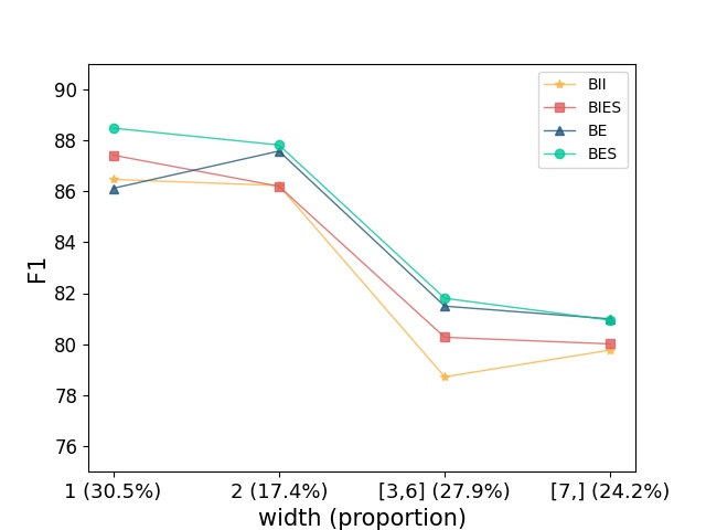
Figure 6: Analysis of the arguments with different width. The horizontal axis denotes the width of arguments and the proportion of arguments of the same width in the data set. The vertical axis denotes the $\mathrm{F}_{1}$ value.

As shown in Figure 6, we divide arguments into four categories according to their width, and report $\mathrm{F}_{1}$ values for each category. The proportion of each category in the gold-standard data is also reported. First, we can see that BES and BIES perform much better on 1-width arguments. This further shows that it is necessary to use “S-$r$” alone to represent arguments of width 1. Then, we can clearly find that BE and BES perform better than BII and BIES on arguments containing multiple words. And we know that BE and BES are resulted from the boundary-attach strategy which pays more attention to boundary information. So, we may conclude that boundary information is more helpful to the recognition of multi-word arguments.

Through analyzing the performance of different schemata, we find that BES is more suitable for converting span-based SRL into word-based graphs than other schemata. So, the rest of the experiments are conducted in BES schema.

6.2 Efficiency

Model	Type	Sents/sec
He et al. (2018)	SGP	44
Strubell et al. (2018)	BIO-based	45
Zhang et al. (2022)	TP	214
Zhang et al. (2022)${}_{\mathrm{\texttt{BERT}}}$		113
Ours	WGP	669
Ours${}_{\mathrm{\texttt{BERT}}}$		252

Table 2: Speed comparison on CoNLL05. “SGP” and “WGP”denote the span-based graph parsing and word-based graph parsing approach respectively; “TP” means the tree parsing approach.

Model	CoNLL05-WSJ				CoNLL05-Brown			CoNLL12
	Dev.$\textrm{F}_{1}$	P	R	$\textrm{F}_{1}$	P	R	$\textrm{F}_{1}$	Dev.$\textrm{F}_{1}$	P	R	$\textrm{F}_{1}$
The end-to-end setting
He et al. (2017)†	80.30	80.20	82.30	81.20	67.60	69.60	68.50	75.50	78.60	75.10	76.80
Strubell et al. (2018)† ∗	81.72	81.77	83.28	82.51	68.58	70.10	69.33	-	-	-	-
He et al. (2018)‡	81.60	81.20	83.90	82.50	69.70	71.90	70.80	79.40	79.40	80.10	79.80
Li et al. (2019)‡	-	-	-	83.00	-	-	-	-	-	-	-
Zhou et al. (2020)	82.27	-	-	-	-	-	-	-	-	-	-
Zhang et al. (2022)	83.91	83.26	86.20	84.71	70.70	74.16	72.39	81.16	79.27	83.24	81.21
Ours	83.17	85.28	83.66	84.46	74.10	70.76	72.39	80.79	82.10	79.76	80.91
Strubell et al. (2018)† ∗ + ELMo	84.73	83.86	85.98	84.91	73.01	75.61	74.31	-	-	-	-
He et al. (2018)‡ + ELMo	85.30	84.80	87.20	86.00	73.90	78.40	76.10	83.00	81.90	84.00	82.90
Li et al. (2019)‡ + ELMo	-	85.20	87.50	86.30	74.70	78.10	76.40	-	84.90	81.40	83.10
Ours + ELMo	85.72	86.19	86.91	86.55	76.57	77.77	77.17	83.72	83.53	83.56	83.54
Zhang et al. (2022) + BERT	87.03	87.00	88.76	87.87	79.08	81.50	80.27	85.53	84.53	86.41	85.45
Ours + BERT	86.79	87.15	88.44	87.79	79.44	80.85	80.14	84.74	83.91	85.61	84.75
The predicate-given setting
He et al. (2017)†	81.60	83.10	83.00	83.10	72.90	71.40	72.10	81.50	81.70	81.60	81.70
Strubell et al. (2018)†	-	84.70	84.24	84.47	73.89	72.39	73.13	-	-	-	-
He et al. (2018)‡	-	-	-	83.90	-	-	73.70	-	-	-	82.10
Tan et al. (2018)†	83.10	84.50	85.20	84.80	73.50	74.60	74.10	82.90	81.90	83.60	82.70
Zhou et al. (2020)	83.16	-	-	-	-	-	-	-	-	-	-
Zhang et al. (2021)	84.45	85.30	85.17	85.23	74.98	73.85	74.41	82.83	83.09	83.71	83.40
Zhang et al. (2022)	84.65	85.47	86.40	85.93	74.92	75.00	74.96	83.39	83.02	84.31	83.66
Ours	84.39	87.01	84.36	85.66	77.86	72.53	75.10	83.83	85.74	82.95	84.32
Li et al. (2019)‡ + ELMo	-	87.90	87.50	87.70	80.60	80.40	80.50	-	85.70	86.30	86.00
Shi and Lin (2019)† + BERT	-	88.60	89.00	88.80	81.90	82.10	82.00	-	85.90	87.00	86.50
Jindal et al. (2020)† + BERT	87.10	87.70	88.00	87.90	80.30	80.10	80.20	86.60	86.30	86.80	86.60
Zhang et al. (2021) + BERT	87.38	87.70	88.15	87.93	81.52	81.36	81.44	86.27	86.00	86.84	86.42
Blloshmi et al. (2021) + BART	-	-	-	-	-	-	-	-	87.80	86.80	87.30
Zhang et al. (2022) + BERT	88.05	89.00	89.03	89.02	82.81	82.35	82.58	87.52	87.52	87.79	87.66
Ours + BERT	87.54	89.03	88.53	88.78	83.22	81.81	82.51	86.97	87.26	87.05	87.15

Table 3: Results on CoNLL05 and CoNLL12 datasets. We mark BIO-based models by $\dagger$ and span-based graph ones by $\ddagger$. For Strubell et al. (2018) and Zhou et al. (2020), we list their syntax-agnostic results to compare fairly. Moreover, we mark the results of Strubell et al. (2018) by ^∗ to indicate that we report corrected evaluation results after re-testing their released models.

Table 2 compares different models in terms of decoding speed. For fair comparison, we re-run all previous models on the same GPU environment (Nvidia GeForce 1080 Ti 11G). The results are averaged over 3 runs. In terms of batch size during evaluation, our model and Strubell et al. (2018) use 5000 tokens (about 134 sentences), while He et al. (2018) and Li et al. (2019) use 40 sentences by default.

We can see that our model improves the efficiency of previous span-based SRL models by large margin. Compared with the span-based graph parsing approach (He et al., 2018; Li et al., 2019), our graph-based parser only has a $O(n^{2})$ search space. As for the BIO-based model of Strubell et al. (2018), the encoder contains $12$ self-attention layers, and they adopts a pipeline framework by first predicting all predicates via sequence labeling and then recognizing arguments, leading to its low parsing speed. And when augmented with BERT, our methods can still parse about 250 sentences per second.

As discussed in Section 2, Zhang et al. (2022) reduce the SRL to a tree parsing task and get good results. However, they have to build a dependency tree for each predicate, which greatly reduces the efficiency of their approach. Specifically, the speed of our model is respectively three and twice times as fast as theirs under the setting without and with BERT.

6.3 Comparison with previous results

End-to-end.

Our work mainly focuses on the end-to-end setting, i.e, requiring predicting predicates and arguments simultaneously. So we first go into this scenario. The first part of the Table 3 shows the comparison with previous works under the end-to-end setting.

First, when compared with models without PLMs, our model surpasses previous approaches with the large gap, getting comparable results with recently released work (Zhang et al., 2022). Then, most previous works usually use ELMo to improve the performance. In order to make a fair comparison, we also report the results with ELMo. We can find that our model also reaches better results, with +0.25 $\textrm{F}_{1}$ on WSJ, +0.77 $\textrm{F}_{1}$ on Brown, and +0.44 $\textrm{F}_{1}$ on CoNLL12-test when using ELMo. And when augmented with the more powerful PLM BERT, the performance of our model can be further improved. It shows that our method not only has high efficiency, but also performs better than previous works.

As discussed in Section 2, please kindly notice that Strubell et al. (2018) and Zhou et al. (2020) use extra syntactic knowledge to boost SRL performance. We only list their syntax-agnostic results here for fair comparison. It is worth noting that Strubell et al. (2018) incidentally wrongly used the official script in the end-to-end setting, leading to much higher precision scores. We reported this issue to their github repository and they confirmed this mistake. In this work, we report their results by evaluating their released models with the correct evaluation process.

Predicate-given.

Recent works (Jindal et al., 2020; Zhang et al., 2021; Blloshmi et al., 2021) usually assume that predicates have been given, thus they only need to recognize the arguments and semantic roles. To compare with these works, we also report the results under the predicate-given setting. In our work, following Cai et al. (2018), during training procedure, the model is informed which word is the predicate using a predicate embedding. The embedding is added to the input vector.

Finally, from the second part of the Table 3, we can see that our model reaches the best results on most test datasets when compared with models without PLMs. When it comes to models with PLMs, we can see that the BIO-based Shi and Lin (2019) is a strong baseline. Our model lags behind them slightly on WSJ, but is much higher than them on other datasets. And even compared with recent seq-to-seq model (Blloshmi et al., 2021), which uses more powerful BART (Lewis et al., 2020), our model still has strong competitiveness.

Comparison with Zhang et al. (2022). As discussed in Section 2, Zhang et al. (2022) propose a tree parsing approach to span-based SRL, which also appears in COLING-2022. We can see that performance of our model is slightly inferior to theirs, possibly due to more careful hyper-parameter tuning according to personal discussion between the two first authors. For example, Zhang confirms that fine-tuning BERT for 20 iterations leads to higher performance, while we only did 10 iterations.

7 Conclusions

This paper proposes four new graph representation schemata for transforming raw span-based SRL structures to word-based graphs. Based on the schema, we cast the span-based SRL as a word-based graph parsing task and present a fast and accurate parser. Moreover, we propose a simple post-processing method based on constrained Viterbi to handle conflicts in the output graphs. Experiments show that our parser 1) is much more efficient than previous parsers, and can parse over 600 sentences per second; 2) reaches consistently better performance than previous results on CoNLL05, CoNLL12 datasets. The in-depth comparison between four schemata shows that the boundary information counts a lot when recognizing arguments. In addition, distinguishing single-word arguments from multi-words arguments can also improve the final performance. These clear findings may help researchers think about SRL from a new perspective in the future.

8 Acknowledgments

We thank our anonymous reviewers for their valuable suggestions. This work was supported by National Natural Science Foundation of China (No. 62176173 and 62076174) and a project funded by the Priority Academic Program Development of Jiangsu Higher Education Institutions.

Appendices

Appendix A More examples of other schemata

In order to save space, we only show the transition matrix of BES in the main body. Here, we present the transition matrix of others in Figure 7. In addition, we provide more examples to improve the comprehensibility of our schemata and the constrained viterbi. Figure 8, 9, and 10 show the outputs of models using different schemata respectively. For example, in Figure 8, there is missing an edge from “pilling” to “falling” in the raw output. After the viterbi procedure, an I-AM-ADV edge will be added since we disallow the transition from O to I-$\ast$. Thus we can get the legal SRL structure.

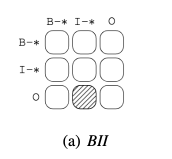
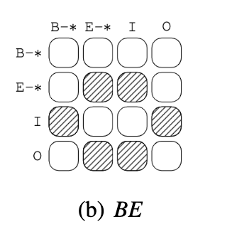
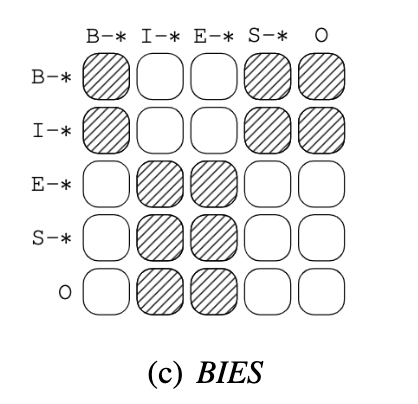
Figure 7: Transition matrices of BII, BE, and BIES.

[arc angle=80] [row sep=0.2cm, column sep=.3cm, font=] Root & pilling & … & while & falling & sharply

[edge style=black,thick]12PRD [edge style=black,thick, edge height=3ex]24B-AM-ADV [edge style=red,dashed, edge height=6ex]25I-AM-ADV [edge style=black,thick, edge height=8ex]26I-AM-ADV

(a) w/o Constrained Viterbi

[arc angle=80] [row sep=0.2cm, column sep=.3cm, font=] Root & pilling & … & while & falling & sharply

[edge style=black,thick]12PRD [edge style=black,thick, edge height=3ex]24B-AM-ADV [edge style=black,thick, edge height=6ex]25I-AM-ADV [edge style=black,thick, edge height=8ex]26I-AM-ADV

(b) w/ Constrained Viterbi

Figure 8: BII schema.

[arc angle=80] [row sep=0.2cm, column sep=.3cm, font=] Root & “ & take & another & … & two & ”

[edge style=black,thick, edge height=3ex]13PRD [edge style=black,thick, edge height=3ex]34B-A1 [edge style=black,thick, edge height=6ex]36E-A1 [edge style=red,thick, edge height=8ex]37E-A1

(a) w/o Constrained Viterbi

[arc angle=80] [row sep=0.2cm, column sep=.3cm, font=] Root & “ & take & another & … & two & ”

[edge style=black,thick, edge height=3ex]13PRD [edge style=black,thick, edge height=3ex]34B-A1 [edge style=black,thick, edge height=6ex]36E-A1

(b) w/ Constrained Viterbi

Figure 9: BE schema.

[arc angle=80] [row sep=0.2cm, column sep=.3cm, font=] Root & fix & … & later & … & when & … & home

[edge style=black,thick]12PRD [edge style=black,thick,edge height=3ex]24B-AM-TMP [edge style=black,thick,edge height=6ex]25I-AM-TMP [edge style=red,thick,edge height=9ex]26B-AM-TMP [edge style=black,thick,edge height=12ex]27I-AM-TMP [edge style=black,thick,edge height=15ex]28E-AM-TMP

(a) w/o Constrained Viterbi

[arc angle=80] [row sep=0.2cm, column sep=.3cm, font=] Root & fix & … & later & … & when & … & home

[edge style=black,thick]12PRD [edge style=black,thick,edge height=3ex]24B-AM-TMP [edge style=black,thick,edge height=6ex]25I-AM-TMP [edge style=black,thick,edge height=9ex]26I-AM-TMP [edge style=black,thick,edge height=12ex]27I-AM-TMP [edge style=black,thick,edge height=15ex]28E-AM-TMP

(b) w/ Constrained Viterbi

Figure 10: BIES schema.

References

- Blloshmi et al. (2021) Rexhina Blloshmi, Simone Conia, Rocco Tripodi, and Roberto Navigli. 2021. Generating senses and roles: An end-to-end model for dependency- and span-based semantic role labeling. In Proceedings of IJCAI, pages 3786–3793.
- Cai et al. (2018) Jiaxun Cai, Shexia He, Zuchao Li, and Hai Zhao. 2018. A full end-to-end semantic role labeler, syntactic-agnostic over syntactic-aware? In Proceedings of ACL, pages 2753–2765.
- Devlin et al. (2019) Jacob Devlin, Ming-Wei Chang, Kenton Lee, and Kristina Toutanova. 2019. Bert: Pre-training of deep bidirectional transformers for language understanding. In Proceedings of NAACL-HLT, pages 4171–4186.
- Dozat and Manning (2018) Timothy Dozat and Christopher D. Manning. 2018. Simpler but more accurate semantic dependency parsing. In Proceedings of ACL, pages 484–490.
- Hajič et al. (2012) Jan Hajič, Eva Hajičová, Jarmila Panevová, Petr Sgall, Ondřej Bojar, Silvie Cinková, Eva Fučíková, Marie Mikulová, Petr Pajas, Jan Popelka, Jiří Semecký, Jana Šindlerová, Jan Štěpánek, Josef Toman, Zdeňka Urešová, and Zdeněk Žabokrtský. 2012. Announcing Prague Czech-English Dependency Treebank 2.0. In Proceedings of LREC, pages 3153–3160.
- He et al. (2018) Luheng He, Kenton Lee, Omer Levy, and Luke Zettlemoyer. 2018. Jointly predicting predicates and arguments in neural semantic role labeling. In Proceedings of ACL, pages 364–369.
- He et al. (2017) Luheng He, Kenton Lee, Mike Lewis, and Luke Zettlemoyer. 2017. Deep semantic role labeling: What works and what’s next. In Proceedings of ACL, pages 473–483.
- Ivanova et al. (2012) Angelina Ivanova, Stephan Oepen, Lilja Øvrelid, and Dan Flickinger. 2012. Who did what to whom? A contrastive study of syntacto-semantic dependencies. In Proceedings of LAW, pages 2–11.
- Jindal et al. (2020) Ishan Jindal, Ranit Aharonov, Siddhartha Brahma, Huaiyu Zhu, and Yunyao Li. 2020. Improved semantic role labeling using parameterized neighborhood memory adaptation. arXiv preprint arXiv:2011.14459.
- Lample et al. (2016) Guillaume Lample, Miguel Ballesteros, Sandeep Subramanian, Kazuya Kawakami, and Chris Dyer. 2016. Neural architectures for named entity recognition. In Proceedings of NAACL-HLT, pages 260–270.
- Lewis et al. (2020) Mike Lewis, Yinhan Liu, Naman Goyal, Marjan Ghazvininejad, Abdelrahman Mohamed, Omer Levy, Veselin Stoyanov, and Luke Zettlemoyer. 2020. BART: Denoising sequence-to-sequence pre-training for natural language generation, translation, and comprehension. In Proceedings of ACL, pages 7871–7880.
- Li et al. (2019) Zuchao Li, Shexia He, Hai Zhao, Yiqing Zhang, Zhuosheng Zhang, Xi Zhou, and Xiang Zhou. 2019. Dependency or span, end-to-end uniform semantic role labeling. In Proceedings of AAAI, pages 6730–6737.
- Li et al. (2020) Zuchao Li, Hai Zhao, Rui Wang, and Kevin Parnow. 2020. High-order semantic role labeling. In Findings of EMNLP, pages 1134–1151.
- Liu and Gildea (2010) Ding Liu and Daniel Gildea. 2010. Semantic role features for machine translation. In Proceedings of COLING, pages 716–724.
- Marcheggiani et al. (2018) Diego Marcheggiani, Jasmijn Bastings, and Ivan Titov. 2018. Exploiting semantics in neural machine translation with graph convolutional networks. In Proceedings of NAACL-HLT, pages 486–492.
- Miyao and Tsujii (2004) Yusuke Miyao and Jun’ichi Tsujii. 2004. Deep linguistic analysis for the accurate identification of predicate-argument relations. In Proceedings of COLING.
- Oepen et al. (2015) Stephan Oepen, Marco Kuhlmann, Yusuke Miyao, Daniel Zeman, Silvie Cinková, Dan Flickinger, Jan Hajic, and Zdenka Uresova. 2015. Semeval 2015 task 18: Broad-coverage semantic dependency parsing. In Proceedings of SemEval, pages 915–926.
- Oepen et al. (2014) Stephan Oepen, Marco Kuhlmann, Yusuke Miyao, Daniel Zeman, Dan Flickinger, Jan Hajič, Angelina Ivanova, and Yi Zhang. 2014. SemEval 2014 task 8: Broad-coverage semantic dependency parsing. In Proceedings of SemEval, pages 63–72.
- Palmer et al. (2005) Martha Palmer, Daniel Gildea, and Paul Kingsbury. 2005. The proposition bank: An annotated corpus of semantic roles. Computational linguistics, 31(1):71–106.
- Pennington et al. (2014) Jeffrey Pennington, Richard Socher, and Christopher Manning. 2014. GloVe: Global vectors for word representation. In Proceedings of EMNLP, pages 1532–1543.
- Peters et al. (2018) Matthew E. Peters, Mark Neumann, Mohit Iyyer, Matt Gardner, Christopher Clark, Kenton Lee, and Luke Zettlemoyer. 2018. Deep contextualized word representations. In Proceedings of NAACL-HLT, pages 2227–2237.
- Pradhan et al. (2012) Sameer Pradhan, Alessandro Moschitti, Nianwen Xue, Olga Uryupina, and Yuchen Zhang. 2012. CoNLL-2012 shared task: Modeling multilingual unrestricted coreference in OntoNotes. In Proceedings of EMNLP-CoNLL, pages 1–40.
- Shi and Lin (2019) Peng Shi and Jimmy Lin. 2019. Simple bert models for relation extraction and semantic role labeling. arXiv preprint arXiv:1904.05255.
- Strubell et al. (2018) Emma Strubell, Patrick Verga, Daniel Andor, David Weiss, and Andrew McCallum. 2018. Linguistically-informed self-attention for semantic role labeling. In Proceedings of EMNLP, pages 5027–5038.
- Tan et al. (2018) Zhixing Tan, Mingxuan Wang, Jun Xie, Yidong Chen, and Xiaodong Shi. 2018. Deep semantic role labeling with self-attention. In Proceedings of AAAI.
- Wang et al. (2015) Hai Wang, Mohit Bansal, Kevin Gimpel, and David McAllester. 2015. Machine comprehension with syntax, frames, and semantics. In Proceedings of ACL-IJCNLP, pages 700–706.
- Wang et al. (2019) Xinyu Wang, Jingxian Huang, and Kewei Tu. 2019. Second-order semantic dependency parsing with end-to-end neural networks. In Proceedings of ACL, pages 4609–4618.
- Xia et al. (2019) Qingrong Xia, Zhenghua Li, Min Zhang, Meishan Zhang, Guohong Fu, Rui Wang, and Luo Si. 2019. Syntax-aware neural semantic role labeling. In Proceedings of AAAI, pages 7305–7313.
- Zhang et al. (2020) Yu Zhang, Zhenghua Li, and Min Zhang. 2020. Efficient second-order TreeCRF for neural dependency parsing. In Proceedings of ACL, pages 3295–3305.
- Zhang et al. (2022) Yu Zhang, Qingrong Xia, Shilin Zhou, Yong Jiang, Guohong Fu, and Min Zhang. 2022. Semantic role labeling as dependency parsing: Exploring latent tree structures inside arguments. In Proceedings of COLING.
- Zhang et al. (2021) Zhisong Zhang, Emma Strubell, and Eduard Hovy. 2021. Comparing span extraction methods for semantic role labeling. In Proceedings of SPNLP, pages 67–77.
- Zhou and Xu (2015) Jie Zhou and Wei Xu. 2015. End-to-end learning of semantic role labeling using recurrent neural networks. In Proceedings of ACL-IJCNLP, pages 1127–1137.
- Zhou et al. (2020) Junru Zhou, Zuchao Li, and Hai Zhao. 2020. Parsing all: Syntax and semantics, dependencies and spans. In Findings of EMNLP, pages 4438–4449.