DANets: Deep Abstract Networks for Tabular Data Classification and Regression

Abstract

Tabular data are ubiquitous in real world applications. Although many commonly-used neural components (e.g., convolution) and extensible neural networks (e.g., ResNet) have been developed by the machine learning community, few of them were effective for tabular data and few designs were adequately tailored for tabular data structures. In this paper, we propose a novel and flexible neural component for tabular data, called Abstract Layer (AbstLay), which learns to explicitly group correlative input features and generate higher-level features for semantics abstraction. Also, we design a structure re-parameterization method to compress the trained AbstLay, thus reducing the computational complexity by a clear margin in the reference phase. A special basic block is built using AbstLays, and we construct a family of Deep Abstract Networks (DANets) for tabular data classification and regression by stacking such blocks. In DANets, a special shortcut path is introduced to fetch information from raw tabular features, assisting feature interactions across different levels. Comprehensive experiments on seven real-world tabular datasets show that our AbstLay and DANets are effective for tabular data classification and regression, and the computational complexity is superior to competitive methods. Besides, we evaluate the performance gains of DANet as it goes deep, verifying the extendibility of our method. Our code is available at https://github.com/WhatAShot/DANet.

Introduction

Data organized in tabular structures, e.g., medical indicators (Hassan et al. 2020; Mirroshandel et al. 2016) and banking records (Roy et al. 2018; Babaev et al. 2019; Addo et al. 2018), are ubiquitous in daily life. However, unlike the boom of deep learning in the computer vision and natural language processing fields, very few neural networks were adequately designed for tabular data (Arik and Pfister 2020; Yang et al. 2018; Ke et al. 2018; Roy et al. 2018; Babaev et al. 2019; Nair and Hinton 2010; Guo, Tang et al. 2017), and hence the performances (e.g., in classification and regression tasks) of such neural networks were still somewhat inferior (Katzir, Elidan et al. 2021). Inspired by the success of ensemble learning (e.g., XGBoost) (Friedman 2001; Chen and Guestrin 2016; Ke et al. 2017; Prokhorenkova et al. 2018; Ho 1995) on tabular data, some recent work resorted to combining multiple neural networks within the framework of ensemble learning (Popov et al. 2019; Katzir, Elidan et al. 2021; Ke et al. 2019). Although ensemble learning can boost the performances of neural networks on tabular data (in the cost of increased computational resources), with such methods, the power of neural networks in tabular feature processing is not yet fully exploited. Besides, there are not many efficient neural components specifically designed for tabular data (analogous to convolution for computer vision). Consequently, known neural networks were mainly based on sundry components and thus were not very extensible.

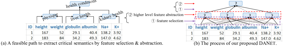
Figure 1: A running example of health assessment for illustrating our insights. (a) A feasible semantics-oriented feature abstraction process. There are three underlying feature groups that can be found to compute high-level features measuring physique, liver health, and kidney health; then these three features are further grouped to estimate the health conditions. (b) An AbstLay  learns a proper feature selection bias to group correlative features and then  abstracts meaningful higher-level features, and DANets organize AbstLays to repeat this process until finally obtaining global semantics for health assessment. The blue rectangles denote the computed high-level features, the grey lines indicate the candidates for feature selection, and the black arrows mark the features eventually selected.

In this paper, we present a flexible neural component called Abstract Layer (AbstLay) for tabular feature abstraction, and build Deep Abstract Networks (DANets) based on AbstLays for tabular data classification and regression. Since tabular features are generally irregular, it is hard to introduce fixed inductive biases (such as dependency among spatially neighboring features in images) in designing neural networks for tabular data processing (e.g., classification and regression). To this end, we assume that there are some underlying feature groups in a tabular data structure, and the features in the groups are correlative and can be exploited to attain higher-level features relevant to the prediction targets. We propose to decouple the process of higher-level tabular feature abstraction into two steps: (i) correlative feature grouping, and (ii) higher-level feature abstraction from grouped features. We employ an AbstLay to perform these two steps, and DANets repeat these two steps by stacking AbstLays to represent critical semantics of tabular data.

Fig. 1 gives a running example to illustrate our insights. As shown in Fig. 1(a), feasible underlying feature groups and the potential feature abstraction paths are organized as follows. The height and weight can be grouped together to compute more comprehensive features that represent the physique. Similarly, features representing liver health and kidney health can be abstracted from the raw features, and the features representing health conditions can further be abstracted from the three high-level features. The semantics are hierarchically aggregated, and the whole process is presented as a parse tree. In contrast, in Fig. 1(b), our method learns to find and group correlative features and then abstract them into higher-level features. This process repeats until global semantics are obtained. The higher-level tabular features are abstracted by one neural layer (AbstLay), and the hierarchical abstraction process is realized with deep learning networks. That is why we call them Abstract Layer and Deep Abstract Networks, respectively.

In designing AbstLay, we contemplate how to group features and abstract them into higher-level features. Since it is hard to find a metric space to measure the feature diversities for feature grouping due to the heterogeneity of tabular data, our AbstLay learns to group the features through employing learnable sparse weight masks, without introducing any explicit distance measurement. Then, subsequent feature learners (in the AbstLay) are utilized to abstract higher-level features from the respective feature groups. Further, motivated by the structure re-parameterization (Ding et al. 2021), we develop a specific re-parameterization method to merge the two step operations of AbstLay into one step in the inference phase, reducing the computational complexity.

Our DANets are built mainly by stacking AbstLays sequentially, and thus tabular features are recursively abstracted layer by layer to obtain the global semantics. To replenish useful features and increase the feature diversity, we also introduce a shortcut path (similar to the residual shortcut (He et al. 2016)), which directly injects the information of raw tabular features into the higher-level features. Specifically, we package the higher-level feature abstraction operation of AbstLay and the feature fetching operation of the shortcut path into a basic block (as specified in Fig. 2(b)), and our DANets are built by stacking such blocks (see Fig. 2(c)). Note that various empirical evidences (He et al. 2016; Qi et al. 2017) have suggested that the successes of deep neural networks (DNNs) are partially benefited from the model depth. Thus, we design DANets with deep architectures, and further discuss the benefits and choices of the model depths by extensive experiments.

In summary, the contributions of this paper are as follows.

• The proposed AbstLay automatically extracts higher-level tabular feature from lower-level ones. AbstLay is simple, and its computational complexity can be reduced in inference by our structure re-parameterization method.

• We introduce a special shortcut path, which fetches raw features for higher levels, promoting the feature diversity for finding meaningful feature groups.

• Based on AbstLays, we build DANets to cope with tabular data classification and regression tasks by recursively abstracting features in order to obtain critical semantics of tabular features.

Related Work

Tabular data processing.

Various conventional machine learning methods (He et al. 2014; Breiman et al. 1984; Chen and Guestrin 2016; Zhang, Kang et al. 2006; Zhang and Honavar 2003) were proposed for tabular data classification and learn-to-rank (regression). Decision tree models (Quinlan 1979; Breiman et al. 1984) can present clear decision paths and are robust on simple tabular datasets. Ensemble models based on decision trees, such as GBDT (Friedman 2001), LightGBM (Ke et al. 2017), XGBoost (Chen and Guestrin 2016), and CatBoost (Prokhorenkova et al. 2018), are currently top choices for tabular data processing, and their performances were comparable (Anghel et al. 2018).

Currently, a research trend aimed to apply DNNs (Guo, Tang et al. 2017; Yang et al. 2018) onto tabular datasets. Some neural networks under the ensemble learning frameworks were presented in (Lay et al. 2018; Feng et al. 2018). Recently, NODE (Popov et al. 2019) combined neural oblivious decision trees with dense connections and obtained comparable performances as GBDTs (Friedman 2001). Net-DNF (Katzir, Elidan et al. 2021) implemented soft versions of logical boolean formulas to aggregate the results of a large number of shallow fully-connected models. Both NODE and Net-DNF essentially followed ensemble learning, employing many (e.g., 2048) shallow neural networks, and thus were computing-complex. Such strategies did not explore the potential of deep models, and their performances should be attributed largely to the number of sub-networks. TabNet (Arik and Pfister 2020) computed sparse attentions sequentially to imitate the sequential feature splitting procedure of tree models. However, TabNet was verified to attain slightly inferior performances, as noted in (Katzir, Elidan et al. 2021).

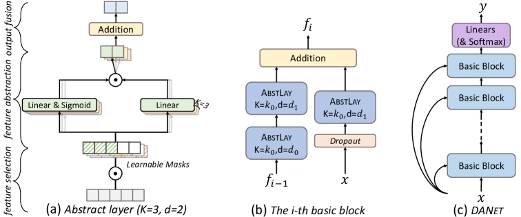
Figure 2: Our proposed architecture for tabular data processing. (a) Illustrating an AbstLay, which performs three steps: feature selection, feature abstracting, and output fusion. In the example of (a), the number of masks, $K$, is set to 3 (see Eq. (3)), the output feature dimension, $d$, is set to 2, and $\odot$ indicates the element-wise multiplication. (b) Illustrating a basic block specification. (c) The architecture of DANet is built mainly by stacking several basic blocks.

Feature selection.

Since tabular features are heterogeneous and irregular, various feature selection methods were applied previously. Classical tree models often used information metrics to guide feature selection, such as information gain (Quinlan 1979), information gain ratio (Quinlan 2014), and Gini index (Breiman et al. 1984), which are essentially greedy algorithms and may require branch pruning (Quinlan 2014) or early stopping strategy. Decision tree ensemble methods often applied random feature sampling to promote diversity. To further assist feature selection, some bagging methods utilized the out-of-bag estimate (James et al. 2013), and gcForest (Zhou and Feng 2017) used sliding windows to scan and group raw features for different forests. A fully-connected neural network (Nair and Hinton 2010) blindly took in all the features, and TabNN (Ke et al. 2018) selected features based on “data structural knowledge” learned by GBDTs. Most of tree models selected one single feature in a step, ignoring the underlying feature correlations.

At present, some neural networks introduced neural operations to select features. NODE (Popov et al. 2019) employed learnable feature selection matrices with Heaviside functions for hard feature selection, imitating the processing of oblivious decision trees. A key to NODE is that the back-propagation optimization is used to replace the information metrics in training the “tree” models. However, the parameters specified by Heaviside functions are hard to update via back-propagation, and thus NODE may take many iterations before convergence. Net-DNF used a straight-through trick (Bengio et al. 2013) to optimize this issue, but it required extra loss functions in training feature selection masks and was inconvenient for users. TabNet (Arik and Pfister 2020) employed an attention mechanism for feature selection, but selected different features for different instances; hence, it is difficult to capture stable feature correlations. In contrast, this paper seeks to find the underlying feature groups representing target-relevant semantics and develop the corresponding operations that are simple and user-friendly.

Problem Statement

Suppose $\mathcal{X}=(\mathcal{F},X,y)$ is one type of specific tabular data structure, where $\mathcal{F}$ specifies the raw feature type space, $X$ is the feasible instance space, and $y$ is the target space. In a tabular dataset of the $\mathcal{X}$ type, an instance $x\in\mathbb{R}^{n}$ in $X$ is defined as an $n$-element vector representing $n$ scalar raw features in $\mathcal{F}$ ($n=\lvert\mathcal{F}\rvert$). Notably, tabular data features are irregular, and the feature permutation in $x$ is predefined. In this paper, we assume that there are some underlying feature groups in a tabular data structure, and the features in a group are correlative and target-relevant. Note that some features may be in no group and some in multiple groups. We are interested in learning mapping functions that take $x\in X$ as input, dig out and address the underlying feature groups for target semantic interests (determined by the classification/regression tasks).

Abstract Layer

Key Functions and Operation

We propose an Abstract layer (AbstLay), which learns to find some underlying feature groups and abstract higher-level features by processing the grouped features. The AbstLay is also desired to be flexible and simple as a basic layer. In our design, the AbstLay comprises feature selection functions to find feature groups, subsequent feature abstracting functions to abstract higher-level features from groups, and an output fusion operation to fuse features abstracted from various groups, as shown in Fig. 2(a).

Feature selection function.

Given an input vector $f\in\mathbb{R}^{m}$ containing $m$ scalar features, a learnable sparse mask $M\in\mathbb{R}^{m}$ selects a subset of scalar features from $f$ for one group. Specifically, this learnable mask is defined as a learnable parameter vector $W_{\text{mask}}$ followed by the Entmax sparsity mapping (Peters et al. 2019), and the features are selected by element-wise multiplying with the sparse mask $M$. The Entmax is a variational form (Wainwright and Jordan 2008) of the Softmax, which introduces sparsity to the output probability. Formally, the feature selection is defined by

$$M=\text{entmax}_{\alpha}(W_{\text{mask}})\ ,\quad f^{\prime}=M\odot f\ ,$$ (1)

where the parameter vector $W_{\text{mask}}\in\mathbb{R}^{m}$, $\odot$ denotes element-wise multiplication, and the selected features are presented in $f^{\prime}\in\mathbb{R}^{m}$. In the Entmax sparsity mapping, we use the default setting with $\alpha=1.5$. With the multiplication, there are some zero values in $f^{\prime}$, and a zero value for the $i$-th scalar feature of the vector $f^{\prime}$ means that the $i$-th scalar feature in $f$ is not selected. This feature selection is simple and can select identical features for different instances.

Feature abstracting function.

Given the selected features in $f^{\prime}\in\mathbb{R}^{m}$ (as defined above), we define the feature abstracting function using a fully connected layer with a simple attention mechanism (Dauphin et al. 2017). Formally, the output $f^{*}$ of a feature abstracting function is computed by

$$q=\text{sigmoid}(\text{BN}(W_{1}f^{\prime}))\ ,\quad f^{*}=\text{ReLU}(q\odot\text{BN}(W_{2}f^{\prime}))\ ,$$ (2)

where the two learnable parameters $W_{c}\in\mathbb{R}^{d\times m}$ ($c=1,2$) are equal-sized, and $q$ denotes the computed attention vector. $W_{c}f^{\prime}$ were implemented by 1D convolutions, and the parametric biases were ignored in Eq.(2). Since tabular data are often trained with a large batch size, we use the ghost batch normalization (Hoffer et al. 2017) to operate “BN”. In this way, the selected features in the vector $f^{\prime}\in\mathbb{R}^{m}$ are projected to $f^{*}\in\mathbb{R}^{d}$, and we treat the $d$ values in the feature vector $f^{*}$ as independent scalar features representing various semantics. Note that all the $d$ features of $f^{*}$ are abstracted from the same group (determined by the same $M$ in Eq. (1)).

Parallel processing and output fusion.

The effect of the AbstLay is realized primarily by the feature selection function and feature abstracting function. These two functions work in sequence to abstract higher-level features from the lower-level feature groups. Yet, we consider that more than one group can be found in a given feature vector $f$. Also, it is common that informative output features are typically obtained by applying some unit operations in parallel (e.g., a convolution layer often contains many kernels). Motivated by these, our AbstLay is designed to find and process multiple low-level feature groups in parallel. Formally, we specify its computation by

$$f_{o}=\sum^{K}_{k=1}p_{k}\circ s_{k}(f)\ ,$$ (3)

where $p\ \circ\ s$ denotes the composite function of a feature selection function $s$ and a feature abstracting function $p$, and $K$ is the number of feature groups that AbstLay manages to get and is a hyper-parameter. We set the output feature sizes of all $p_{k}\circ s_{k}$ identical. The output features of all the composite functions $p_{k}\circ s_{k}$ are element-wise added to form the output features $f_{o}$ of AbstLay (see Fig. 2(a)).

Similar to the convolution layers in a model, several AbstLays can be stacked together and operate as a whole. Thus, the output scalar features of one AbstLay may be further grouped by its subsequent AbstLay for further information abstraction, and the useless output features from the preceding AbstLay can be abandoned. Different from the complicated “feature transformation” function in TabNet (Arik and Pfister 2020), the ability of the AbstLays is largely due to their co-operation (e.g., layer-by-layer processing).

AbstLay Complexity Reduction

To reduce the computational complexity of our proposed AbstLay, we develop a re-parameterization method following (Ding et al. 2021) to reformulate the AbstLays. Note that $W_{1}\in\mathbb{R}^{d\times m}$ and $W_{2}\in\mathbb{R}^{d\times m}$ are weights of feature abstracting function, and $M\in\mathbb{R}^{m}$ is also a weight vector. Substituting Eq. (1) into Eq. (2), we have

$$q=\text{sigmoid}(\text{BN}(W_{1}(M\odot f)))\ ,$$ (4)

$$f^{*}=\text{ReLU}(q\odot\text{BN}(W_{2}(M\odot f)))\ .$$

Thus, we can use $W_{c}^{\prime}\in\mathbb{R}^{d\times m}$ to replace the multiplication term $W_{c}M$ ($c=1,2$) in Eq. (4), by

$$W_{c}^{\prime}[:,j]=W_{c}[:,j]*M[j]\ ,$$

where $j=1,2,\ldots,m$, and $m$ is the input feature dimension. Besides, we can further merge the batch normalization operation into the weights $W^{\prime}_{c}$, by

$$W^{*}_{c}[i,:]=\frac{\gamma[i]}{\sigma[i]}W_{c}^{\prime}[i,:]\ , b^{*}_{c}[i]=(\beta[i]-\frac{\mu[i]\gamma[i]}{\sigma[i]})\ ,$$ (5)

where $i=1,2,\ldots,d$ and $d$ is the output feature dimension, $\gamma\in\mathbb{R}^{d}$ and $\beta\in\mathbb{R}^{d}$ are the learnable parameters of the batch normalization followed $W_{c}$ (the formula is $z^{\prime}=\frac{\gamma}{\sigma}z+(\beta-\frac{\mu\gamma}{\sigma})$ for a feature vector $z$), and $\mu\in\mathbb{R}^{d}$ and $\sigma\in\mathbb{R}^{d}$ are the computed mean and standard deviation. Then, the operation in an AbstLay (see Eq. (3)) can be simplified as

$$f_{o}=\sum^{K}_{k=1}\text{ReLU}(\text{sigmoid}(W^{*}_{k,1}f+b^{*}_{k,1})\odot(W^{*}_{k,2}f+b^{*}_{k,2}))\ ,$$ (6)

where $W^{*}_{k,c}$ ($c=1,2$) is the weights $W^{*}_{c}$ re-parameterized by Eq. (5) for the $k$-th feature abstracting function in an AbstLay (see Eq. (3), an AbstLay has $K$ functions), and $b^{*}_{k,c}$ is the $b^{*}_{c}$ in Eq.(5) for the $k$-th feature abstracting function. In this way, a lighter model can be used in inference by re-parameterization.

Deep Abstract Networks

Based on the proposed AbstLay, we introduce Deep Abstract Networks (DANets) for tabular data processing. DANets stack AbstLays to repeatedly find and process some meaningful feature groups for higher-level feature abstraction. Besides, we allow features in different levels to be grouped together, thus increasing the model capability. Hence, we design a new shortcut path that allows a high-level layer to fetch raw features. Specifically, we propose a basic block based on AbstLays containing the shortcut path, and our DANets are built by sequentially stacking such blocks.

A Basic Block

Our basic block is mainly built using AbstLays, and a new shortcut can add features abstracted from the groups of raw features to the main model path. Fig. 2(b) illustrates the specification of the basic block in DANets. Formally, we define the $i$-th basic block $f_{i}$ by

$$f_{i}=\mathcal{G}_{i}(f_{i-1})+g_{i}(x)\ ,$$ (7)

where $g_{i}$ is the shortcut consists of an AbstLay and a Dropout layer (Srivastava et al. 2014) and takes raw features $x$ as input. The term $\mathcal{G}_{i}$ is on the main path containing multiple AbstLays and its input is the features produced by the previous basic block (see Fig. 2(c)). For the first basic block $f_{1}$, we let $f_{0}=x$. Unlike the residual block in ResNet (He et al. 2016) whose shortcut path brings the features of the preceding layers, our shortcut fetches the raw features.

In a DANet with many basic blocks (see Fig. 2(c)), the combination of $\mathcal{G}_{i}$’s of the basic blocks acts as the main path of the model, which extracts and forwards target-relevant information. The target-relevant information is replenished continuously via the shortcut terms $g_{i}$ of the basic blocks. From Fig. 2(c), it is obvious that a raw feature can be used by a high-level basic block via a shortcut directly, while the information of some raw features may be taken by a higher-level layer through the main path after the layer-by-layer processing. Thus, the feature diversity in a layer increases compared to a layer in a model without such shortcuts. Notably, we include a Dropout operation in the shortcut path, which encourages the subsequent AbstLay to focus on the core information that the basic block requires.

Table 1: A summary of the seven public datasets. The datasets marked with “†” are randomly split into training and test sets by a ratio of 8:2. (“Forest”: “Forest Cover Type”; “Cardio.”: “Cardiovascular Disease”; “L2R”: “Learn to Rank”; “Clas.”: “Classification”.)

Datasets	YearPrediction	Microsoft	Yahoo	Epsilon	Click	Cardio.†	Forest†
# Features	90	136	699	2K	11	11	54
Size of train data	463K	723K	544K	400K	900K	56K	400K
Size of test data	51.6K	241K	165K	100K	100K	14K	100K
Task types	L2R	L2R	L2R	Clas.	Clas.	Clas.	Clas.
Metric	MSE	MSE	MSE	Acc.	Acc.	Acc.	Acc.

Table 2: Performance comparison on the seven tabular datasets. The best performances are marked in orange, and the second and third best ones are marked in blue and green, respectively. Note that for classification tasks, a better method gets a higher accuracy, and for learn-to-rank tasks, a better method gets a lower MSE.

Methods	Rank	Classification				Learn-to-rank
		Forest	Cardio.	Epsilon	Click	Microsoft	YearP.	Yahoo
XGBoost (Chen and Guestrin 2016)	4	97.13%$\pm$2e-4	73.97%$\pm$2e-4	88.89%$\pm$6e-4	66.66%$\pm$2e-3	0.5544$\pm$1e-4	78.53$\pm$0.09	0.5420$\pm$4e-4
CatBoost (Prokhorenkova et al. 2018)	5	95.67%$\pm$4e-4	74.02%$\pm$1e-4	88.87%$\pm$4e-4	65.99%$\pm$2e-3	0.5565$\pm$2e-4	79.67$\pm$0.12	0.5632$\pm$3e-4
gcForest (Zhou and Feng 2017)	–	96.29%	73.27%	88.21%	66.67%	–	–	–
Net-DNF (Katzir, Elidan et al. 2021)	–	97.21%$\pm$2e-4	73.75%$\pm$2e-4	88.23%$\pm$3e-4	66.94%$\pm$4e-4	–	–	–
TabNet (Arik and Pfister 2020)	7	96.99%$\pm$8e-4	73.70%$\pm$6e-4	89.65%$\pm$8e-5	66.84%$\pm$2e-4	0.5707$\pm$3e-4	77.36$\pm$0.37	0.5925$\pm$1e-3
NODE (Popov et al. 2019)	3	96.95%$\pm$3e-4	73.93%$\pm$7e-4	89.66%$\pm$3e-4	66.88%$\pm$2e-3	0.5570$\pm$2e-4	76.21$\pm$0.12	0.5692$\pm$2e-4
FCNN (Nair and Hinton 2010)	8	96.83%$\pm$1e-4	73.86%$\pm$4e-4	89.59%$\pm$2e-4	66.75%$\pm$2e-3	0.5608$\pm$4e-4	79.99$\pm$0.47	0.5773$\pm$1e-3
FCNN + $l^{1}$-norm	5	96.85%$\pm$1e-3	73.90%$\pm$5e-4	89.49%$\pm$2e-3	67.01%$\pm$2e-4	0.5694$\pm$1e-3	76.52$\pm$0.02	0.6016$\pm$1e-3
DANet-20 (ours)	2	97.23%$\pm$2e-4	74.04%$\pm$5e-4	89.58%$\pm$4e-4	67.11%$\pm$2e-4	0.5550$\pm$7e-4	76.76$\pm$0.15	0.5678$\pm$4e-4
DANet-32 (ours)	1	97.27%$\pm$5e-4	73.98%$\pm$2e-4	89.67%$\pm$2e-4	67.19%$\pm$5e-4	0.5557$\pm$3e-4	75.93$\pm$0.17	0.5703$\pm$6e-5

Network Architectures and Training

We stack the basic blocks in sequence to build a DANet architecture, as shown in Fig. 2(c). In our setting, we fix the basic block specification that contains three AbstLays, as shown in Fig. 2(b). That is, in Eq. (7), $\mathcal{G}_{i}$ is composed of two AbstLays, and $g_{i}$ contains one. Then, a three-layer MLP (a multi-layer perceptron network) with ReLU activation is used at the end of a DANet for classification (with Softmax) or regression. We have tested various network architecture specifications, and observed consistent patterns. Here, we present some concrete architectures, such as DANet-20 and DANet-32, to analyze the effects of DANets.

Similar to the previous DNNs for tabular data (Arik and Pfister 2020; Popov et al. 2019), our DANets can deal with classification and learn-to-rank (regression) tasks on tabular data. DANets are trained with the specification of the Cross-Entropy loss function for classification, and are trained with the mean squared error (MSE) for regression. Note that the feature names are not used in this paper.

Experiments

In this section, we present extensive experiments to compare the effects of our DANets and the known state-of-the-art models. Also, we present several empirical studies to analyze the effects of some critical DANet components, including the learnable sparse masks, shortcut paths, model depth, and model width (the $K$ value in Eq. (3)). Besides, we evaluate the effects of our proposed sparse masks on correlative feature grouping using three synthesized datasets.

Experimental Setup

Datasets.

We conduct experiments on seven open-source tabular datasets: Microsoft (Qin and Liu 2013), YearPrediction (Bertin-Mahieux et al. 2011), and Yahoo (Mohan et al. 2011) for regression; Forest Cover Type, Click, Epsilon, and Cardiovascular Disease for classification. The details of the datasets are listed as in Table 1. Most of the datasets provide train-test splits. For Click, we follow the train-test split provided by the open-source of NODE (Popov et al. 2019). In all the experiments, we fix the train-test split for fair comparison. For the tasks on learning to rank, we use regression similar to the previous work. For Click, the categorical features were pre-processed with the Leave-One-Out encoder of the scikit-learn library. We used the official validation set of every dataset if it is given. On the datasets that do not provide official validation sets, we stratified to sample $20\%$ of instances from the full training datasets for validation.

Implementation details.

We implement our various DANet architectures with PyTorch on Python 3.7. All the experiments are run on NVIDIA Tesla V100. In training, the batch size is 8,192 with the ghost batch size 256 in the ghost batch normalization layers, and the learning rate is initially set to $0.008$ and is decayed by $5\%$ in every 20 epochs. The optimizer is the QHAdam optimizer (Ma and Yarats 2019) with default configurations except for the weight decay rate $10^{-5}$ and discount factors $(0.8,1.0)$. For the other methods, the performances are obtained with their specific settings. Unlike previous methods requiring carefully setting their hyper-parameters (e.g., NODE (Popov et al. 2019)), we fix the primary setting of DANets: We set $k_{0}=5$, $d_{0}=32$, and $d_{1}=64$ as default (see Fig. 2(b)). For the datasets with large amounts of raw features (e.g., Yahoo with 699 features and Epsilon with 2K features), we set $k_{0}=8$, $d_{0}=48$, and $d_{1}=96$. We use the dropout rate $0.1$ for all the datasets except for Forest Cover Type without using dropout. The performances of the other methods are hyperparameter-tuned for best possible results using the Hyperopt library and performed 50 steps of the Tree-structured Parzen Estimator (TPE) optimization algorithm, similar to the settings in (Popov et al. 2019). We set the hyper-parameter search spaces and search algorithms of XGBoost (Chen and Guestrin 2016), CatBoost (Prokhorenkova et al. 2018), NODE (Popov et al. 2019), and FCNN (Nair and Hinton 2010) as in (Popov et al. 2019), while the hyperparameter search settings of Net-DNF (Katzir, Elidan et al. 2021) and TabNet (Arik and Pfister 2020) followed their original papers. The hyperparameters of gcForest (Zhou and Feng 2017) followed its default values. The architectures of FCNN with or without $l^{1}$-norm regularization were constructed following the FCNN in (Popov et al. 2019). The hyper-parameters of these compared methods are selected according to the validation performances, and the performances are obtained on the corresponding test sets.

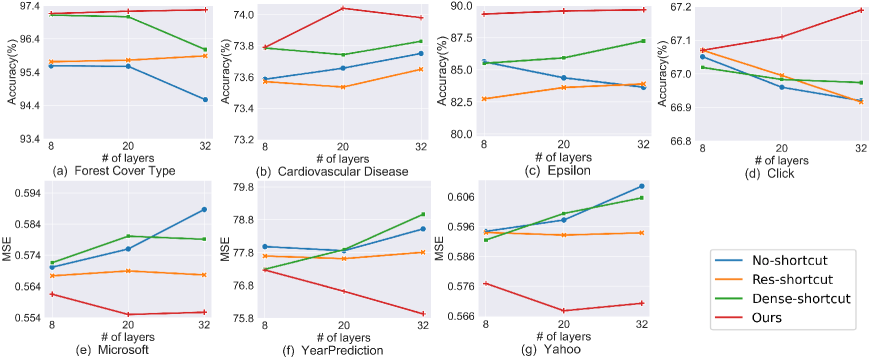
Figure 3: The performances on various datasets with different kinds of shortcuts. For classification (shown in (a), (b), (c), and (d)), the higher accuracy, the better. For regression (shown in (e), (f), and (g)), the lower MSE, the better. It is obvious that our shortcuts are superior.

Comparison baselines.

To evaluate the performances, we compare our DANet-20 and DANet-32 with several common conventional methods, including XGBoost (Chen and Guestrin 2016), gcForest (Zhou and Feng 2017), and CatBoost (Prokhorenkova et al. 2018), and the best-known neural networks, including TabNet (Arik and Pfister 2020), FCNN (Nair and Hinton 2010) with and without the $l^{1}$-norm regularization, and NODE (Popov et al. 2019).

Results and Analyses

Performance comparison.

The comparison performances on the seven tabular datasets are reported in Table 2. One can see that our methods (i.e., DANet-20 and DANet-32) outperform or are comparable with the previous neural networks and GBDTs. Note that the parameters of our DANets are pre-set, while the other methods are specifically hyperparameter-tuned for each dataset. This implies that our DANets are not only better-performing but also easy-to-use. Further, we rank all the methods (except gcForest (Zhou and Feng 2017) and Net-DNF (Katzir, Elidan et al. 2021), since they can only work on classification) based on the averaged performance ranks on the datasets, and our methods DANet-20 and DANet-32 attain the best performances among all the methods. Besides, the overall performances of DANet-32 are better than DANet-20, obtaining performance gain by increasing the model depth.

The effects of shortcuts.

A key design of our DANets is the special shortcut connections in the basic blocks. To inspect the effects of our proposed shortcuts, we compare DANets with the models with conventional residual shortcuts (Res-shortcut), the models without any shortcuts, and the models with densely connected shortcuts (Dense-shortcut) (Huang et al. 2017). For fairness, we only replace our shortcuts with other shortcuts in DANet-8, DANet-20, and DANet-32. The performances are shown in Fig. 3. It is evident that DANets with our shortcuts significantly outperform the models with other shortcuts in all the model depth specifications. Besides, one might see that the effects of our proposed shortcuts are more evident in most the cases with deeper DANets. For example, in Fig. 3(b), (d), (e), (f), and (g), the performance differences on DANet-32 are more noticeable than those on DANet-8. This might be because information can be efficiently replenished via our shortcuts, thus helping promote the effectiveness of the deeper models.

Table 3: The mask activation on three synthesized datasets. Each heatmap has two rows: The top row is for the mask in the main model path, and the bottom row is for the mask in the shortcut path.

Formulas	Learn-to-rank	Classification
$y=\sum^{5}_{i=2}(v^{2}_{i})$
$y=|\log{|v_{0}-v_{2}|}+\cos{(v_{5}+\sin{v_{6}})-(10^{-8}\times v_{10})}|$
$y=\sum\limits_{(i,j)\in{\{(6,7),(5,8)\}}}{-10}\sin{\frac{(v_{i}+v_{j})}{10}}+(v_{i}+v_{j})^{2}$
$y=$ if $v_{1}<0$; $y=$ if $v_{1}>0$

The effects of model depth.

We show the effects of the DANet model depths on the Forest Cover Type dataset in Fig. 4, and we also examined similar phenomena on the other datasets. From Fig. 4, one can see that DANets yield better performances with increasing model depths. However, when DANets get very deep (e.g., deeper than DANet-32), the performance gain becomes diminutive. We think this is because tabular data usually have much fewer features than image/text data for very deep networks to exploit. We observe that for DANets, the depths of 20–32 are promising choices.

The effects of model width.

The number of feature groups, $K$, in an AbstLay acts as the model width for DANets. To evaluate the effect of the width $K$, we show the performances of DANet-20 with different widths on Click (11 features), Forest Cover Type (54 features), and Epsilon (2K features) in Table 4. DANet-20 yields considerable performances with width $K=5$. For the datasets with less features (e.g., Click and Forest Cover Type), we only see slight gains with width $K>5$. For the dataset with more features (Epsilon), $K=8$ seems to be a reasonable choice, which outperforms $K=5$ by $0.13\%$. This may be because a dataset with more features tends to have more feature groups, and thus a larger model width may help in such scenarios.

The effects of sparse masks.

We inspect the effects of the masks on three synthesized datasets with three different dataset settings. Each dataset contains $7k$ input items with 11 scalar features ($x=\{v_{i}|i=0,\ldots,10\}$) generated from an $11$-dimensional Gaussian distribution without feature correlation. Four formulas are used to compute the target $y$ in the first column of Table 3. As for the learn-to-rank tasks, $y$ is used as the prediction targets; as for the classification tasks, $y$ is further transformed into “0” or “1” using the median of $y$ as the threshold value. We build an DANet-2 with $K=1$, and train it with the synthesized datasets. This model has only one basic block, and there are two masks whose input is the raw features (i.e., the mask of the first AbstLay in the main model path and the mask of the AbstLay in the shortcut). In this study, we only inspect these two masks after training to convergence, and check whether the mask activation matches the formulas. The mask activation is visualized in Table 3.

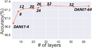
Figure 4: DANet performances in different model depths on Forest Cover Type.

Table 4: DANet-20 performances with different widths.

$K$	Click	Forest	Epsilon
1	67.03%	96.18%	89.13%
5	67.11%	97.23%	89.45%
8	67.12%	97.21%	89.58%
14	67.15%	97.22%	89.61%
20	67.15%	97.23%	89.63%

Taking the learn-to-rank tasks as example, our first question is: Can our masks distinguish the target-relevant and target-irrelevant features? For Formula , one can see that only the features $v_{2},v_{3},v_{4}$, and $v_{5}$ are target-relevant, and the corresponding values in the masks are highly responding to them. Similar results can be seen in the other cases. Especially, we introduce a term with regard to $v_{10}$ tending to zero in Formula , and one can see that the masks do not respond to it, which shows that our proposed mask is data-driven and robust. Our second question is: Can our masks group correlative features? In Formula , we can regard $v_{0}$ and $v_{2}$ as in one group, and $v_{5}$ and $v_{6}$ as in another group. We can see that in the masks, the values representing $v_{0}$ and $v_{2}$ have close values, and so do $v_{5}$ and $v_{6}$. In Formula , there are two feature groups: $(v_{6},v_{7})$ and $(v_{5},v_{8})$. Correspondingly, a mask “selects” $v_{6}$ and $v_{7}$, and the other one “selects” $v_{5}$ and $v_{8}$. As for the piecewise function in Formula , $v_{1}$ (as a condition) and all the features used in Formulas and are considered by the masks. In summary, one can see that our proposed masks not only can find target-relevant features, but also have the ability to dig out feature relations. Similar conclusions can be drawn for the classification tasks.

Computational complexity comparison.

We compare the computational complexities in the inference phases of DANets with the performance-competitive neural networks, TabNet, NODE (Popov et al. 2019), and Net-DNF (Katzir, Elidan et al. 2021) (see Fig. 5). The FLOPS of ensemble learning based methods (i.e., NODE and Net-DNF) are generally several times those of DANets and TabNet. Besides, it is obvious that, under some identical complexities, our models are often the best-performed ones. Seeing the grey curve in Fig. 5, TabNet cannot obtain the performance gains when keeping enlarging the model size, which are not very extensible compared to ours. After model compression by the structure re-parameterization performed on AbstLays, the FLOPS of our DANets are reduced by $14.8\%$–$23.0\%$ (compared the red and green curves). As for one single AbstLay, the FLOPS are reduced by $49.02\%$ with the input and output feature sizes of 32.

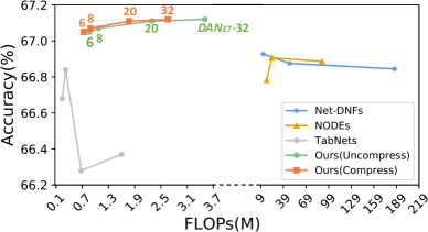
Figure 5: The computational complexity comparison on the Click dataset among DANets and other methods.

Conclusions

In this paper, we proposed a family of parse-tree-like deep neural networks, DANets, for tabular learning. We designed a novel neural component, AbstLay, for tabular data, which automatically selects correlative features and abstracts higher-level features from the grouped features. We also provided a structure re-parameterization method which can largely reduce the computational complexity of AbstLay. We developed a basic block based on AbstLays, and DANets in various depths were built by stacking such blocks. A special shortcut in the basic block was introduced, increasing the diversity of feature groups. Experiments on several public datasets verified that our DANets are effective and efficient in processing tabular data, for both classification and learn-to-rank tasks. Besides, using synthesized datasets, we show that the proposed masks can find feature correlations. Besides, the ablation studies explored the effectiveness of model depths and widths, which suggested that a wider and deeper DANet is beneficial but the extreme depth and width architectures were not recommended due to the limited spaces of tabular features.

References

- Addo et al. (2018) Addo, P. M.; et al. 2018. Credit risk analysis using machine and deep learning models. Risks.
- Anghel et al. (2018) Anghel, A.; et al. 2018. Benchmarking and optimization of gradient boosting decision tree algorithms. In NeurIPS.
- Arik and Pfister (2020) Arik, S. O.; and Pfister, T. 2020. TabNet: Attentive interpretable tabular learning. In AAAI.
- Babaev et al. (2019) Babaev, D.; et al. 2019. E.T.-RNN: Applying deep learning to credit loan applications. In KDD.
- Bengio et al. (2013) Bengio, Y.; et al. 2013. Estimating or propagating gradients through stochastic neurons for conditional computation. arXiv preprint arXiv:1308.3432.
- Bertin-Mahieux et al. (2011) Bertin-Mahieux, T.; et al. 2011. The million song dataset. In ISMIR.
- Breiman et al. (1984) Breiman, L.; et al. 1984. Classification and Regression Trees. CRC press.
- Chen and Guestrin (2016) Chen, T.; and Guestrin, C. 2016. XGBoost: A scalable tree boosting system. In KDD.
- Dauphin et al. (2017) Dauphin, Y. N.; et al. 2017. Language modeling with gated convolutional networks. In ICML.
- Ding et al. (2021) Ding, X.; et al. 2021. RepVGG: Making VGG-style ConvNets great again. In CVPR.
- Feng et al. (2018) Feng, J.; et al. 2018. Multi-layered gradient boosting decision trees. In NeurIPS.
- Friedman (2001) Friedman, J. H. 2001. Greedy function approximation: A gradient boosting machine. Annals of Statistics.
- Guo, Tang et al. (2017) Guo, H.; Tang, R.; et al. 2017. DeepFM: A factorization-machine based neural network for CTR prediction. In IJCAI.
- Hassan et al. (2020) Hassan, M. R.; et al. 2020. A machine learning approach for prediction of pregnancy outcome following IVF treatment. Neural Computing and Applications.
- He et al. (2016) He, K.; et al. 2016. Deep residual learning for image recognition. In CVPR.
- He et al. (2014) He, X.; et al. 2014. Practical lessons from predicting clicks on Ads at Fackbook. In DMOA Workshop.
- Ho (1995) Ho, T. K. 1995. Random decision forests. In ICDAR.
- Hoffer et al. (2017) Hoffer, E.; et al. 2017. Train longer, generalize better: Closing the generalization gap in large batch training of neural networks. In NeurIPS.
- Huang et al. (2017) Huang, G.; et al. 2017. Densely connected convolutional networks. In CVPR.
- James et al. (2013) James, G.; et al. 2013. An Introduction to Statistical Learning. Springer.
- Katzir, Elidan et al. (2021) Katzir, L.; Elidan, G.; et al. 2021. DNF-Net: Effective deep modeling of tabular data. In ICLR.
- Ke et al. (2017) Ke, G.; et al. 2017. LightGBM: A highly efficient gradient boosting decision tree. In NeurIPS.
- Ke et al. (2018) Ke, G.; et al. 2018. TabNN: A universal neural network solution for tabular data. In ICLR OpenReview.
- Ke et al. (2019) Ke, G.; et al. 2019. DeepGBM: A deep learning framework distilled by GBDT for online prediction tasks. In KDD.
- Lay et al. (2018) Lay, N.; et al. 2018. Random hinge forest for differentiable learning. In ICML.
- Ma and Yarats (2019) Ma, J.; and Yarats, D. 2019. Quasi-hyperbolic momentum and Adam for deep learning. In ICLR.
- Mirroshandel et al. (2016) Mirroshandel, S. A.; et al. 2016. Applying data mining techniques for increasing implantation rate by selecting best sperms for intra-cytoplasmic sperm injection treatment. Computer Methods and Programs in Biomedicine.
- Mohan et al. (2011) Mohan, A.; et al. 2011. Web-search ranking with initialized gradient boosted regression trees. In Proceedings of the Learning to Rank Challenge.
- Nair and Hinton (2010) Nair, V.; and Hinton, G. E. 2010. Rectified linear units improve restricted Boltzmann machines. In ICML.
- Peters et al. (2019) Peters, B.; et al. 2019. Sparse sequence-to-sequence models. In ACL.
- Popov et al. (2019) Popov, S.; et al. 2019. Neural oblivious decision ensembles for deep learning on tabular data. In ICLR.
- Prokhorenkova et al. (2018) Prokhorenkova, L.; et al. 2018. CatBoost: Unbiased boosting with categorical features. In NeurIPS.
- Qi et al. (2017) Qi, C. R.; et al. 2017. PointNet++: Deep hierarchical feature learning on point sets in a metric space. In NeurIPS.
- Qin and Liu (2013) Qin, T.; and Liu, T. 2013. Introducing LETOR 4.0 Datasets. CoRR.
- Quinlan (1979) Quinlan, J. R. 1979. Discovering rules by induction from large collections of examples. Expert Systems in the Micro Electronics Age.
- Quinlan (2014) Quinlan, J. R. 2014. C4.5: Programs for Machine Learning. Elsevier.
- Roy et al. (2018) Roy, A.; et al. 2018. Deep learning detecting fraud in credit card transactions. In Systems and Information Engineering Design Symposium.
- Srivastava et al. (2014) Srivastava, N.; et al. 2014. Dropout: A simple way to prevent neural networks from overfitting. JMLR.
- Wainwright and Jordan (2008) Wainwright, M. J.; and Jordan, M. I. 2008. Graphical Models, Exponential Families, and Variational Inference. Now Publishers Inc.
- Yang et al. (2018) Yang, Y.; et al. 2018. Deep neural decision trees. In ICML Workshop.
- Zhang and Honavar (2003) Zhang, J.; and Honavar, V. 2003. Learning from attribute value taxonomies and partially specified instances. In ICML.
- Zhang, Kang et al. (2006) Zhang, J.; Kang, D.-K.; et al. 2006. Learning accurate and concise naïve Bayes classifiers from attribute value taxonomies and data. Knowledge and Information Systems.
- Zhou and Feng (2017) Zhou, Z.-H.; and Feng, J. 2017. Deep Forest: Towards an alternative to deep neural networks. In IJCAI.