Phase shift in periodically driven non-equilibrium systems: Its identification and a bound

Abstract

Time-dependently driven stochastic systems form a vast and manifold class of non-equilibrium systems used to model important applications on small length scales such as bit erasure protocols or microscopic heat engines. One property that unites all these quite different systems is some form of lag between the driving of the system and its response. For periodic steady states, we quantify this lag by introducing a generalized phase difference and prove a tight upper bound for it. In its most general version, this bound depends only on the relative speed of the driving.

Keywords: lag, phase, periodic steady state

1 Introduction

Recent technological advancements allowing a precise manipulation and fabrication on the micro- and nanoscale led to a growing interest in small stochastic non-equilibrium systems in which fluctuations play a fundamental role. Time-dependently driven systems constitute the arguably largest and most diverse class of such non-equilibrium systems containing a variety of systems such as microscopic heat engines [1, 2, 3, 4, 5, 6, 7], applications of bit erasure processes [8, 9, 10, 11], stochastic pumps [12, 13, 14, 15, 16], as well as biological or chemical systems exposed to time-dependent stimuli, see, e.g., Refs. [17, 18]. One common property of such time-dependently driven systems is some form of lag between the driving and the response of the system. Time-dependent driving is generally accompanied by a change in the instantaneous steady state to which the system tends to relax. The relaxation is not immediate and inevitably leads to a lag or delay between the system and its driving. Previously, this lag has been quantified by comparing the time-dependent probability density with the instantaneous steady state leading to relations about dissipated work and drift [19, 20].

Exact solutions for non-equilibrium systems are rarely feasible, even less so for time-dependently driven systems. However, major progress has been achieved by establishing inequalities and bounds for various dynamic quantities. One vast family of bounds are the so-called thermodynamic uncertainty relations [21], which cover a wide range of different system classes such as non-equilibrium steady states [22, 23], systems relaxing to equilibrium [24, 25], periodically driven systems [26, 27, 28, 29] or arbitrarily driven systems [30, 31]. Besides the thermodynamic uncertainty relations speed limits [32, 33, 34, 35, 36] form another large group of bounds. The general idea of these speed limits is often related to the aforementioned notion of lag since there are inherent limitations for the speed of certain processes due to ”inertia” of these systems.

It is often desirable to minimize the lag in time-dependently driven systems. For example, biological systems need to readily adapt to changing circumstances. A fast response to changing concentrations of nutrients can pose a significant advantage for the organism [37]. Another example can be found among measuring devices, such as molecular sensors. For many applications they need to operate with small lag [38].

In this paper, we address the question of quantifying the lag in periodically driven systems. As a first main result, we introduce a quantity that measures the lag in a Markov network, for which the energy of each state varies periodically. In contrast to the approach in Refs. [19, 20] this quantity is not time-dependent but rather poses a phase difference between the driving and the response of the system. As the second main result of this paper, we will prove a universal upper bound on this phase that only depends on the speed at which the system is driven.

2 Setup

We consider a discrete Markovian system with $N$ states. The time evolution of the probability $p_{i}(t)$ to find the system in state $i$ at time $t$ is governed by the master equation

$$\partial_{t}p_{i}(t)=-\sum_{j\neq i}\left[p_{i}(t)k_{ij}(t)-p_{j}(t)k_{ji}(t)\right],$$ (1)

where $k_{ij}(t)$ denotes the transition rate between states $i$ and $j$. The transition rates must fulfill the local detailed balance relation in order to model the system in a thermodynamically consistent way. They are parametrized as

$$k_{ij}(t) =k_{0,ij}e^{\alpha_{ij}\Delta E_{ij}(t)},$$ (2)

$$k_{ji}(t) =k_{0,ij}e^{-(1-\alpha_{ij})\Delta E_{ij}(t)}$$ (3)

with time-dependent energy difference $\Delta E_{ij}(t)\equiv E_{i}(t)-E_{j}(t)$. The parameter $\alpha_{ij}\in\left[0,1\right]$ determines its splitting in forward and backward rate. The rate amplitude $k_{0,ij}$ sets the time scale of the transition. We set $k_{B}T=1$ throughout this paper. The system is driven by periodically varying the energies

$$E_{i}(t)=E_{i}^{0}+E\sum_{n}\left[c^{n}_{i}\sin\left(n\Omega t\right)+d^{n}_{i}\cos\left(n\Omega t\right)\right]$$ (4)

for each state $i$ with the frequency $\Omega=2\pi/\mathcal{T}$. The energy amplitude $E$ sets the general scale of the driving and allows us to keep the Fourier coefficients $\left\{c_{i}^{n},d_{i}^{n}\right\}$ of the order of $1$. The parameters $E_{i}^{0}$ are the constant energy offsets. In the long-time limit, the system will reach the periodic steady state $p_{i}^{\mathchoice{\hbox{{ps}}}{\hbox{{ps}}}{\hbox{{ps}}}{\hbox{{ps}}}}(t)=p_{i}^{\mathchoice{\hbox{{ps}}}{\hbox{{ps}}}{\hbox{{ps}}}{\hbox{{ps}}}}(t+\mathcal{T})$. In the following, we will focus on this periodic steady state and omit the superscript $p_{i}(t)\equiv p_{i}^{\mathchoice{\hbox{{ps}}}{\hbox{{ps}}}{\hbox{{ps}}}{\hbox{{ps}}}}(t)$.

The framework of stochastic thermodynamics allows us to identify thermodynamic quantities, such as heat, work and entropy production [39]. Since we consider the periodic steady state, we focus on the rates of these quantities averaged over one period. The rate of work, i.e. power, applied to state $i$ is defined as

$$P_{i}\equiv\frac{1}{\mathcal{T}}\int_{0}^{\mathcal{T}}{\mathchoice{\hbox{{d}}}{\hbox{{d}}}{\hbox{{d}}}{\hbox{{d}}}}tp_{i}(t)\partial_{t}E_{i}(t).$$ (5)

The total entropy production rate in these systems is identical to the medium entropy production rate, since the stochastic entropy production vanishes in the average over one period, which leaves us with

$$\sigma\equiv\frac{1}{\mathcal{T}}\int_{0}^{\mathcal{T}}{\mathchoice{\hbox{{d}}}{\hbox{{d}}}{\hbox{{d}}}{\hbox{{d}}}}t\sum_{i,j}p_{i}(t)k_{ij}(t)\ln\left(\frac{k_{ij}(t)}{k_{ji}(t)}\right).$$ (6)

The entropy production rate is equal to the heat flux in the system and due to conservation of energy we have

$$\sigma=\sum_{i=1}^{N}P_{i}.$$ (7)

3 Definition of the phase for a two-state system

First, we identify the phase that quantifies the lag in a two-state system. In this case there is only one timescale $k_{0}$ for the transitions and one energy difference $\Delta E(t)$, which determines the driving. To motivate the definition of the phase, we first consider a general Fourier series with coefficients $\left\{f_{n},g_{n}\right\}$. Such a Fourier series can also be expressed in terms of amplitudes $\left\{A_{n}\right\}$ and phases $\left\{\Phi_{n}\right\}$

$$\sum_{n}f_{n}\sin\left(n\Omega t\right)+g_{n}\cos\left(n\Omega t\right)=\sum_{n}A_{n}\sin\left(n\Omega t+\Phi_{n}\right)$$ (8)

with

$$\Phi_{n} =\left\{\begin{array}[]{lr}\arctan\left(g_{n}/f_{n}\right),&{\mathchoice{\hbox{{for }}}{\hbox{{for }}}{\hbox{{for }}}{\hbox{{for }}}}f_{n}\geq 0\\ \arctan\left(g_{n}/f_{n}\right)-\pi,&{\mathchoice{\hbox{{for }}}{\hbox{{for }}}{\hbox{{for }}}{\hbox{{for }}}}f_{n}<0\end{array}\right..$$ (11)

The phase $\Phi_{n}$ follows from the coefficients of the Fourier series and denotes the phase difference between the terms of the Fourier series and, in this case, $\sin\left(n\Omega t\right)$.

Similarly, the idea behind our definition of the phase that quantifies the lag in the periodic steady state of a two-state system is to expand the probability $p_{1}(t)$ into a Fourier-like series

$$p_{1}(t)=\sum_{n}a_{n}v_{n}(t)+b_{n}w_{n}(t)$$ (12)

with basis functions $\left\{v_{n}(t),w_{n}(t)\right\}$ and coefficients $\left\{a_{n},b_{n}\right\}$. The two crucial basis functions are $v_{1}(t)$ and $w_{1}(t)$, which we choose as functions of the driving (4). The ratio of the corresponding coefficients defines a phase analogous to equation (11). This phase can be interpreted as a phase difference between the driving and the response of the system expressed in terms of $p_{1}(t)$. All further basis vectors appearing in the series (12) complement $v_{1}(t)$ and $w_{1}(t)$ so that $\left\{v_{n}(t),w_{n}(t)\right\}$ defines a complete and orthogonal basis for functions with periodicity $\mathcal{T}$.

We now need to find suitable choices for the functions $v_{1}(t)$ and $w_{1}(t)$. Since the phase is supposed to quantify a lag, slow driving $\Omega/k_{0}\to 0$ is expected to minimize this quantity and fast driving $k_{0}/\Omega\to 0$ is expected to maximize it. To fulfill these criteria, the coefficients $b_{1}$ and $a_{1}$ need to vanish in the limit of slow driving and in the limit of fast driving, respectively. We start with the first case. In the quasistatic limit $p_{1}(t)$ converges to the instantaneous equilibrium distribution

$$p_{1}(t)=p_{1}^{{\mathchoice{\hbox{{qs}}}{\hbox{{qs}}}{\hbox{{qs}}}{\hbox{{qs}}}}}(t)=\frac{1}{1+e^{\Delta E(t)}}$$ (13)

with $\Delta E(t)\equiv\Delta E_{12}(t)$. The condition that the coefficient $b_{1}$ vanishes for slow driving is equivalent to $w_{1}(t)$ being orthogonal to $p_{1}^{{\mathchoice{\hbox{{qs}}}{\hbox{{qs}}}{\hbox{{qs}}}{\hbox{{qs}}}}}(t)$

$$\int_{0}^{\mathcal{T}}p_{1}^{{\mathchoice{\hbox{{qs}}}{\hbox{{qs}}}{\hbox{{qs}}}{\hbox{{qs}}}}}(t)w_{1}(t){\mathchoice{\hbox{{d}}}{\hbox{{d}}}{\hbox{{d}}}{\hbox{{d}}}}t=\int_{0}^{\mathcal{T}}\frac{1}{1+e^{\Delta E(t)}}w_{1}(t){\mathchoice{\hbox{{d}}}{\hbox{{d}}}{\hbox{{d}}}{\hbox{{d}}}}t\stackrel{{\scriptstyle!}}{{=}}0.$$ (14)

This condition suggests the choice $w_{1}(t)\equiv\partial_{t}\Delta E(t)/N_{2}$ with an arbitrary constant $N_{2}$. The integral (14) becomes zero with this choice, since the integrand is a function of the periodic $\Delta E(t)$ multiplied with its derivative $\partial_{t}\Delta E(t)$. Any integral over one period $\mathcal{T}$ of an integrand $f\left(g(t)\right)\partial_{t}{g}(t)$ with periodic function $g(t)=g(t+\mathcal{T})$ vanishes as shown through a substitution $t\to u=g(t)$. With this choice the integral (14) becomes proportional to the entropy production $\sigma$, which generically vanishes in the limit of slow driving. Thus, we have found the first basis function $w_{1}(t)$.

Finding $v_{1}(t)$ is slightly more involved. The criterion for $a_{1}$ to vanish in the limit of fast driving translates into the condition that $v_{1}(t)$ is orthogonal to $p_{1}(t)$ in the limit $k_{0}/\Omega\to 0$. To calculate the leading orders of $p_{1}(t)$ in $k_{0}/\Omega$, we use a perturbative expansion of the probability

$$p_{1}(\tau)=p_{1}^{(0)}(\tau)+\frac{k_{0}}{\Omega}p_{1}^{(1)}(\tau)+\mathcal{O}\left(\frac{k_{0}^{2}}{\Omega^{2}}\right)$$ (15)

with dimensionless time variable $\tau\equiv\Omega t$. Inserting (15) into the master equation (1) yields

$$\partial_{\tau}p_{1}^{(0)}(\tau) =0,$$ (16)

$$\partial_{\tau}p_{1}^{(1)}(\tau) =-\left[\tilde{k}_{12}(\tau)+\tilde{k}_{21}(\tau)\right]p_{1}^{(0)}(\tau)+\tilde{k}_{21}(\tau)$$ (17)

with $\tilde{k}_{ij}(t)=k_{ij}(t)/k_{0}$. Equation (16) shows that the zeroth order is time-independent. Thus, we consider the integral

$$\int_{0}^{\mathcal{T}}p_{1}^{(1)}(t)v_{1}(t){\mathchoice{\hbox{{d}}}{\hbox{{d}}}{\hbox{{d}}}{\hbox{{d}}}}t=-\int_{0}^{2\pi}\partial_{\tau}p_{1}^{(1)}(\tau)V_{1}(\tau){\mathchoice{\hbox{{d}}}{\hbox{{d}}}{\hbox{{d}}}{\hbox{{d}}}}\tau$$

$$=\int_{0}^{2\pi}\left[\left(\tilde{k}_{12}(\tau)+\tilde{k}_{21}(\tau)\right)p_{1}^{(0)}(\tau)-\tilde{k}_{21}(\tau)\right]V_{1}(\tau){\mathchoice{\hbox{{d}}}{\hbox{{d}}}{\hbox{{d}}}{\hbox{{d}}}}\tau\stackrel{{\scriptstyle!}}{{=}}0$$ (18)

with $\partial_{t}V_{1}(t)=v_{1}(t)$. Since $p_{1}^{(0)}(\tau)$ is a constant in time, the expression in square brackets in the integral (18) is a function of $\Delta E(\tau)$ only. This suggests the choice $V_{1}(\tau)=\partial_{\tau}\Delta E(\tau)/N_{1}$, which translates into $v_{1}(t)=\partial_{t}^{2}\Delta E(t)/(N_{1}\Omega)$ with arbitrary constant $N_{1}$ with similar reasoning as previously discussed for slow driving. To summarize, we have found the suitable first two basis functions

$$v_{1}(t) =\frac{\partial_{t}^{2}\Delta E(t)}{N_{1}\Omega}\;\;\;\;\;\;{\mathchoice{\hbox{{and}}}{\hbox{{and}}}{\hbox{{and}}}{\hbox{{and}}}}\;\;\;\;\;\;w_{1}(t) =\frac{\partial_{t}\Delta E(t)}{N_{2}}.$$ (19)

These basis functions lead to our first main result. Analogous to equation (11), the phase can be identified as

$$\Delta\varphi=\arctan\left(\frac{b_{1}}{a_{1}}\right)=\arctan\left(\frac{\langle\partial_{t}E(t)\rangle\Omega}{\langle\partial_{t}^{2}{E}(t)\rangle}\right).$$ (20)

Here, we have chosen the constants

$$N_{1}=\frac{1}{\mathcal{T}}\int_{0}^{\mathcal{T}}\frac{\left(\partial_{t}^{2}\Delta E(t)\right)^{2}}{\Omega^{2}}{\mathchoice{\hbox{{d}}}{\hbox{{d}}}{\hbox{{d}}}{\hbox{{d}}}}t\;\;\;\;\;\;{\mathchoice{\hbox{{ and }}}{\hbox{{ and }}}{\hbox{{ and }}}{\hbox{{ and }}}}\;\;\;\;\;\;N_{2}=\frac{1}{\mathcal{T}}\int_{0}^{\mathcal{T}}\left(\partial_{t}\Delta E(t)\right)^{2}{\mathchoice{\hbox{{d}}}{\hbox{{d}}}{\hbox{{d}}}{\hbox{{d}}}}t$$ (21)

such that the coefficients are given by

$$a_{1}=\frac{1}{\mathcal{T}}\int_{0}^{\mathcal{T}}p_{1}(t)\frac{\partial_{t}^{2}\Delta E(t)}{\Omega}{\mathchoice{\hbox{{d}}}{\hbox{{d}}}{\hbox{{d}}}{\hbox{{d}}}}t=\langle\partial_{t}^{2}{E}(t)\rangle/\Omega$$ (22)

and

$$b_{1}=\frac{1}{\mathcal{T}}\int_{0}^{\mathcal{T}}p_{1}(t)\partial_{t}\Delta E(t){\mathchoice{\hbox{{d}}}{\hbox{{d}}}{\hbox{{d}}}{\hbox{{d}}}}t=\langle\partial_{t}E(t)\rangle.$$ (23)

The average $\langle\cdot\rangle$ is defined over many realizations and over one period as

$$\langle X_{i}\rangle\equiv\sum_{i=1}^{N}\frac{1}{\mathcal{T}}\int_{0}^{\mathcal{T}}p_{i}(t)X_{i}(t){\mathchoice{\hbox{{d}}}{\hbox{{d}}}{\hbox{{d}}}{\hbox{{d}}}}t.$$ (24)

Furthermore, $b_{1}$ is the total applied power (5) and, hence, coincides with the total entropy production rate (6). We note that the second case of equation (11) can be omitted in equation (20) since $a_{1}$ and $b_{1}$ are both positive as shown in A. Equation (20) shows that in the limit of slow driving $\Delta\varphi$ vanishes due to $b_{1}=0$. For fast driving, the phase approaches its maximum with $\Delta\varphi=\pi/2$ due to $a_{1}=0$.

We now consider the simplest non-trivial case of a single driving frequency to get a better understanding of the quantity $\Delta\varphi$. The driving can be written as

$$\Delta E(t)=\Delta E_{0}+E\sin\left(\Omega t\right)$$ (25)

with $\Delta E_{0}\equiv E^{0}_{1}-E^{0}_{2}$. In this case, the series in equation (12) reduces to a Fourier series, since ${v_{1}(t)=-2\sin\left(\Omega t\right)/(E\Omega)}$ and ${w_{1}(t)=2\cos\left(\Omega t\right)/(E\Omega)}$. The quantity $\Delta\varphi$ is then the ordinary phase difference between the driving $\Delta E(t)$ and the probability $p_{1}(t)$ at the frequency of the driving as illustrated in Figure 1. The example demonstrates the geometric aspect that is related to the delay in a periodically driven system. In the more general case of an arbitrary number of driving frequencies the idea of expressing the probability in terms of the driving remains the same.

Figure 1: Illustration of the phase $\Delta\varphi$ for the case of a single driving frequency (25). The green and blue lines show the periodic stationary state as a function of time for one period. The red line shows the first order of the series (12) shifted along the $y$-axis by a constant offset. The dashed line indicates the driving $\Delta E(t)$ scaled along the $y$-axis. The phase $\Delta\varphi$ as defined in (20) is the difference between the extremum of the driving and the extremum of $a_{1}v_{1}(t)+b_{1}w_{1}(t)$.

Notably, the phase difference does not scale with the amplitude of the driving $\Delta E(t)$ or the probability $p_{1}(t)$, neither in the aforementioned simplest case (25), nor in the general case (4). However, there is an indirect dependence, because the amplitude of $\Delta E(t)$ influences the shape of the probability $p_{1}(t)$ and, therefore, also the phase. Two functions $A\Delta E(t)$ and $Bp_{1}(t)$ yield the same value of $\Delta\varphi$ independently of the arbitrary constants $A$ and $B$. This is in contrast to the definition of lag in Refs. [19, 20] where small amplitudes inevitably lead to a small lag. However, the lag does not necessarily vanish for weak driving. As it turns out it rather becomes maximal as we will discuss in section 4. We argue that this phase $\Delta\varphi$, which allows a lag of the order of $1$ even for small driving, is a meaningful way of quantifying the physical lag.

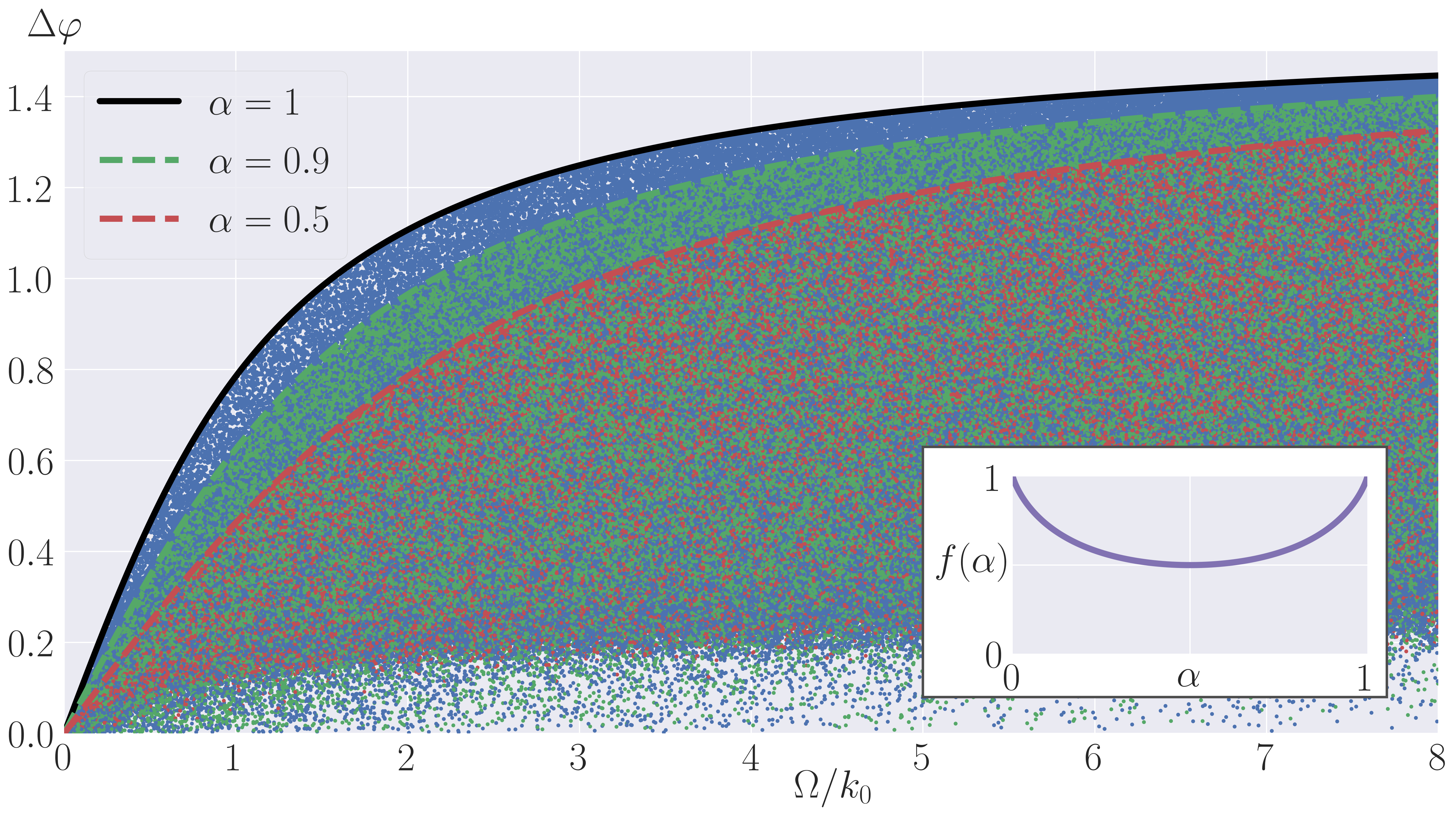
Figure 2: Illustration of the bounds (26) and (27). The colors indicate the value of $\alpha$; blue: $\alpha\in\left\{0,1\right\}$, green: $\alpha\in\left\{0.1,0.9\right\}$, red: $\alpha=0.5$. For each system the parameters are drawn randomly from uniform distributions with $\alpha\in\left\{0,0.1,0.5,0.9,1\right\}$, $E\in\left[0,4\right]$, $\Omega/k_{0}\in\left[0.01,8\right]$, $c_{i}^{n},d_{i}^{n}\in\left[-1,1\right]$ and $E_{i}^{0}\in\left[-4,4\right]$. The solid black line shows the bound (26). The dashed blue and green lines show the bound (27) for $\alpha=0.5$ and $\alpha=0.9$ respectively. The inset shows the $\alpha$ dependency of the bound (27).

4 Bounds on the phase

Our second main result is an upper bound on the phase,

$$\Delta\varphi\leq\arctan\left(\frac{\Omega}{k_{0}}\right),$$ (26)

that depends only on the relative speed of the driving and holds for arbitrary periodic driving (4) in a two-state system. Since $\Omega$ determines the time scale of the driving and $k_{0}$ the time scale at which transitions in the system occur, the ratio of these two quantities gives an effective speed of driving. Figure 2 illustrates the quality of this bound through numerical results. Each dot represents the numerically calculated phase $\Delta\varphi$ in a system with randomly chosen parameters. Obviously, the bound (26) can be saturated for any relative driving speed $\Omega/k_{0}$.

The information about the relative speed of the driving alone, encoded in the parameter $\Omega/k_{0}$, is sufficient to bound the lag $\Delta\varphi$. However, by including additional information, specifically about the distribution of the rates in forward and backward rate as quantified by the parameter $\alpha$, a stronger bound follows as

$$\Delta\varphi\leq\arctan\left(f\left(\alpha\right)\frac{\Omega}{k_{0}}\right)\leq\arctan\left(\frac{\Omega}{k_{0}}\right)$$ (27)

with

$$f\left(\alpha\right)\equiv\alpha^{\alpha}\left(1-\alpha\right)^{1-\alpha}\leq 1$$ (28)

for all $\alpha\in\left[0,1\right]$. For any $\alpha$ in the relevant interval $\left[0,1\right]$, the relation $1/2\leq f\left(\alpha\right)\leq 1$ applies. More specifically, $f\left(\alpha\right)$ is maximized at the boundaries $\alpha=0,1$ and minimized at the center $\alpha=1/2$ while being monotonous in between and symmetrical with respect to the center, see inset of Figure 2. The stronger bound is illustrated for a few values of $\alpha$ in Figure 2.

For a proof of these bounds, it is sufficient to derive the more detailed bound (27), from which the main result (26) follows due to $f\left(\alpha\right)\leq 1$, the positivity of the arguments of the arctan-function and its monotonicity. To derive the bound (27), we consider the putative inequality

$$\gamma\langle\partial_{t}^{2}E(t)\rangle/\Omega-\langle\partial_{t}E(t)\rangle\geq 0$$ (29)

with the additional free parameter $\gamma$. Any choice for $\gamma$ that fulfills the inequality (29) implies a bound of the form

$$\Delta\varphi\leq\arctan\gamma,$$ (30)

due to (20). To obtain the best bound, we optimize with respect to $\gamma$ while still preserving the inequality (29) as further detailed in A. This procedure leads to the optimal value of $\gamma$ given by

$$\gamma^{*}=f\left(\alpha\right)\frac{\Omega}{k_{0}},$$ (31)

which implies the bound (27) by using (30). To summarize, we have derived two bounds on the phase $\Delta\varphi$, one general bound, which only depends on the relative speed of the driving and one more detailed bound that additionally takes information about the rate splitting into account.

As the numerical data shown in Figure 2 demonstrates, the bound (27) can be saturated for any relative driving speed $\Omega/k_{0}$. We now discuss the conditions leading to saturation. Saturating the bound is equivalent to constructing a system with maximum lag. As shown in detail in B, the two key parameters to construct such a system are the amplitude of the driving $E$ and the energy offset $\Delta E_{0}$. Remarkably, the exact form of the driving defined through its Fourier coefficients (4) does not matter in this case. The energy amplitude needs to be small $E\ll 1$, leading to an overall weak driving in a linear response regime. The energy offset has to be chosen according to the splitting of the rates as

$$\Delta E_{0}=\log\left(\frac{1-\alpha}{\alpha}\right).$$ (32)

Qualitatively, both of these conditions are expected for a system with maximum lag. The system always relaxes towards the instantaneous equilibrium state but ultimately always lags behind. The speed at which it relaxes and, therefore, tries to follow the instantaneous equilibrium state is determined by the transition rates. While the transition rates scale exponentially with the amplitude $E$ of the driving, the instantaneous equilibrium state has a weaker scaling, especially since it is limited to values between $0$ and $1$. Thus, a high energy amplitude generally reduces the lag or, conversely, a low energy amplitude generally leads to a higher lag.

The energy offset $\Delta E_{0}$ that leads to the maximum lag depends on the splitting parameter $\alpha$. The splitting determines which rate is more sensitive to the energy difference between the states. Choosing $\alpha$ close to $1$ implies that $k_{12}(t)$ is more sensitive than $k_{21}(t)$ and vice versa for $\alpha$ close to $0$. A positive $\Delta E_{0}$ increases the rate $k_{12}(t)$ and decreases the rate $k_{21}(t)$, whereas a negative $\Delta E_{0}$ has the opposing effect on the rates. To maximize the lag, the energy offset $\Delta E_{0}$ has to increase the rate that is less dependent on the energy difference and decrease the rate that is more dependent on it. In the extreme cases of $\alpha=0,1$ one rate does not scale with the energy difference at all. Here, $\Delta E_{0}$ diverges with the expected sign, as shown by equation (32).

5 $N$-state system

In this section, we consider an arbitrary Markov network with $N$ states. We aim to generalize the definition of the phase to quantify the inherent lag in any periodically driven Markov network. Multiple challenges arise when dealing with these more complex systems. First, the driving cannot be described by a single scalar quantity comparable to $\Delta E(t)$. Instead, there are individual energy differences for all links of the system. Second, there is no single characteristic time scale of the system. The local detailed balance relation allows one to have different rate amplitudes $k_{0,ij}$ for every link. Third, similar to the rate amplitudes, local detailed balance also allows for a different splitting of rates $\alpha_{ij}$ at any available link.

In the definitions (22) and (23) we have written the coefficients as averages of the second and first derivative of the energies. A natural generalization of the definitions in (20), (22) and (23) is to keep these notions and apply the general average

$$a_{1}(N) =\frac{\langle\partial_{t}^{2}{E}(t)\rangle}{\Omega}=\sum_{i=1}^{N}\int_{0}^{\mathcal{T}}p_{i}(t)\frac{\partial_{t}^{2}{E}_{i}(t)}{\Omega}{\mathchoice{\hbox{{d}}}{\hbox{{d}}}{\hbox{{d}}}{\hbox{{d}}}}t=\int_{0}^{\mathcal{T}}\mathbf{p}(t)\cdot\partial_{t}^{2}{\mathbf{E}}(t)\frac{1}{\Omega}{\mathchoice{\hbox{{d}}}{\hbox{{d}}}{\hbox{{d}}}{\hbox{{d}}}}t,$$ (33)

$$b_{1}(N) =\langle\partial_{t}E(t)\rangle=\sum_{i=1}^{N}\int_{0}^{\mathcal{T}}p_{i}(t)\partial_{t}E_{i}(t){\mathchoice{\hbox{{d}}}{\hbox{{d}}}{\hbox{{d}}}{\hbox{{d}}}}t=\int_{0}^{\mathcal{T}}\mathbf{p}(t)\cdot\partial_{t}{\mathbf{E}}(t){\mathchoice{\hbox{{d}}}{\hbox{{d}}}{\hbox{{d}}}{\hbox{{d}}}}t$$ (34)

with

$$\textbf{p}(t)=\left(p_{1}(t),\cdots,p_{N}(t)\right)^{T}$$ (35)

and

$$\textbf{E}(t)=\left(E_{1}(t),\cdots,E_{N}(t)\right)^{T}$$ (36)

to obtain a similar expression

$$\Delta\varphi=\arctan\left(\frac{b_{1}(N)}{a_{1}(N)}\right)$$ (37)

for the phase. The interpretation of expressing the phase in terms of the driving still remains valid. However, the driving is now described by an $N$-component vector instead of a scalar quantity.

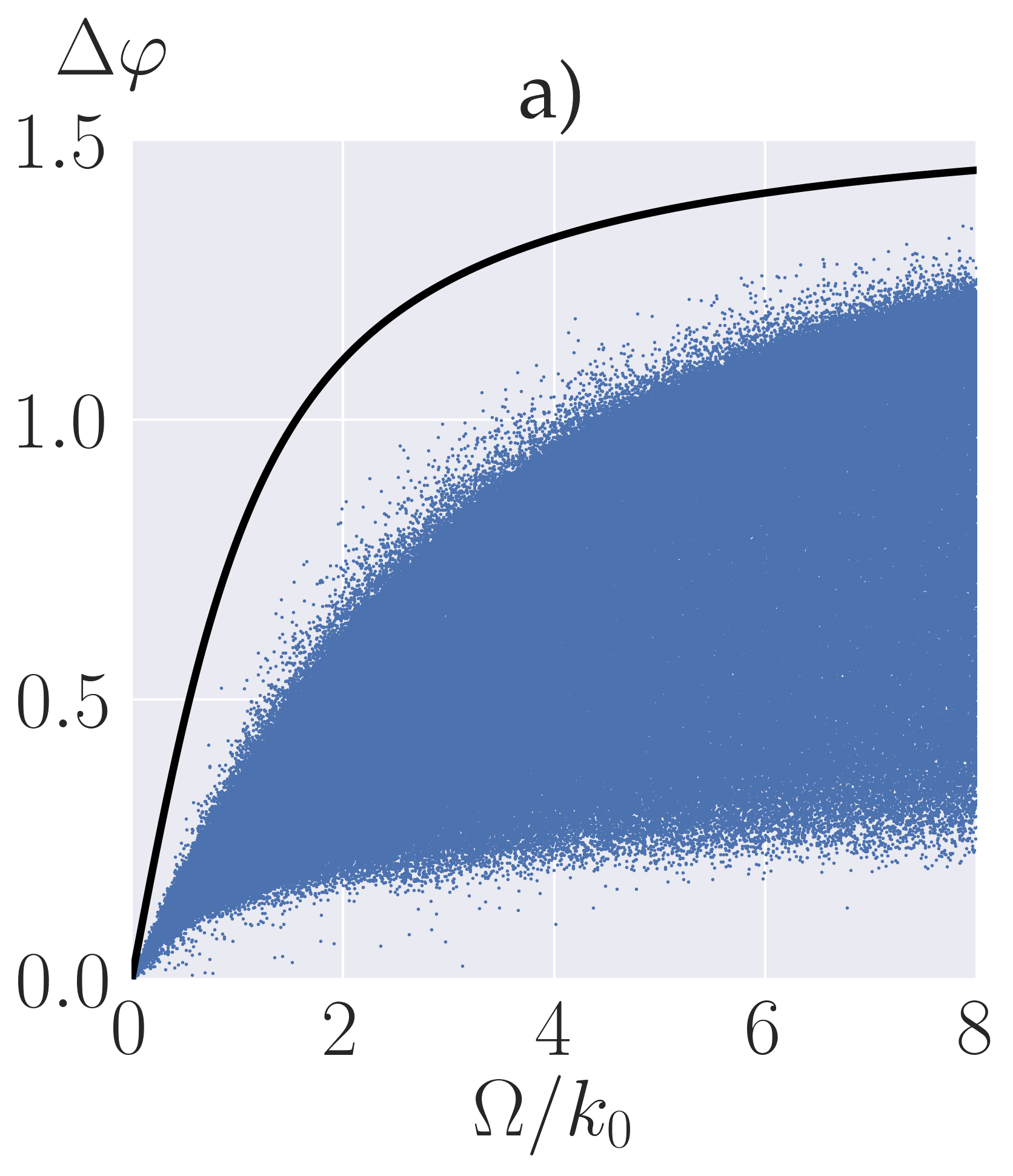
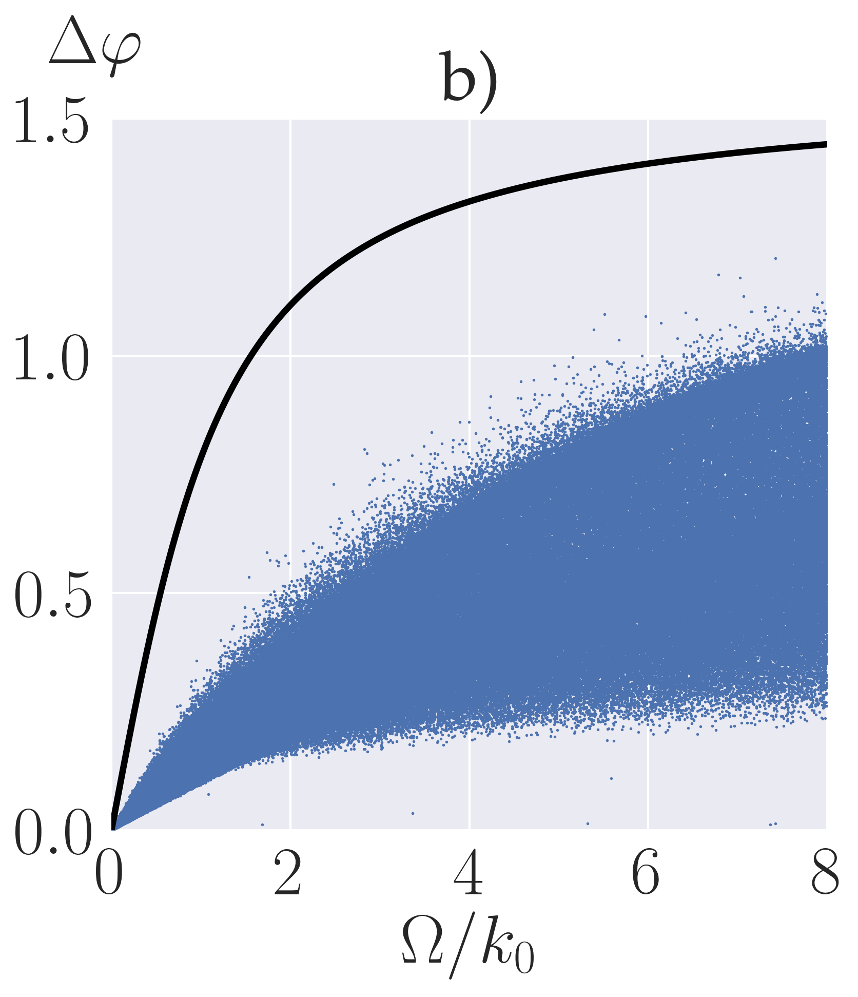
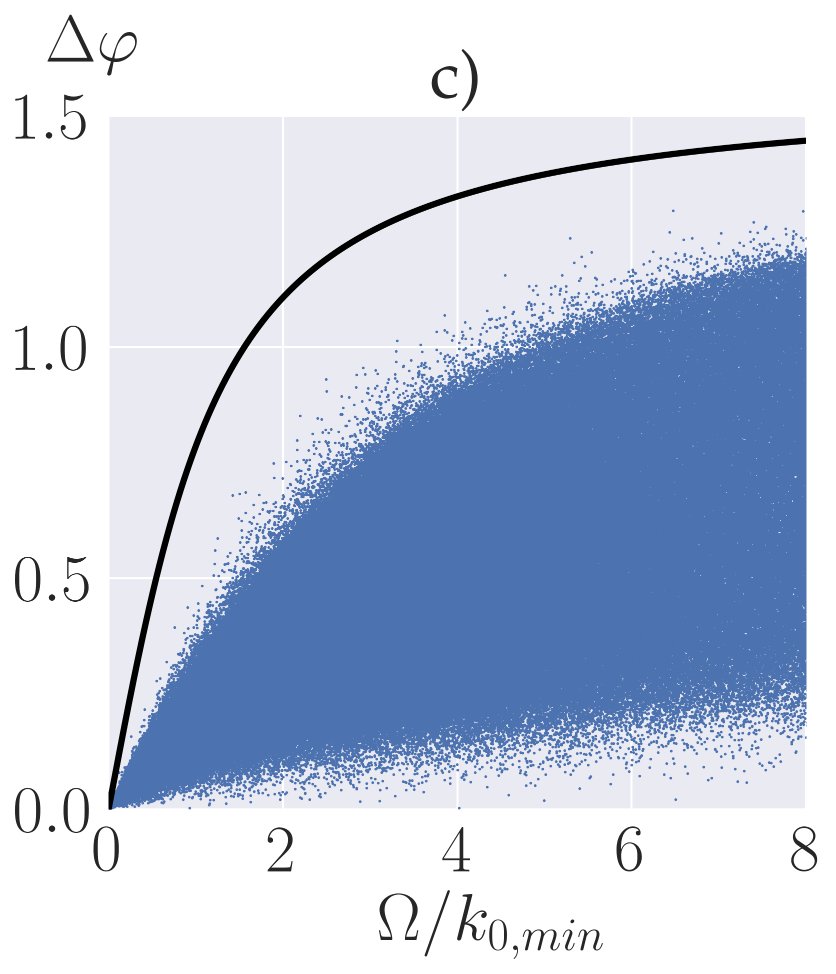
Figure 3: Illustration of the bound (26) for the phase (37) for $N$-state systems. Each point represents the numerically calculated phase of a system in dependence of the relative driving speed. For each system the numerical parameters $\alpha_{ij}\in\left[0,1\right]$, $E\in\left[0,4\right]$, $c_{i}^{n},d_{i}^{n}\in\left[-1,1\right]$ and $E_{i}^{0}\in\left[-4,4\right]$ are drawn randomly from uniform distributions. a) $N=3$ state systems with common rate amplitude $k_{0}$. $\Omega/k_{0}\in\left[0.01,8\right]$ is drawn from a uniform distribution. b) $N=5$ and $N=10$ state systems with common rate amplitude $k_{0}$. $\Omega/k_{0}\in\left[0.01,8\right]$ is drawn from a uniform distribution. c) $N=3$ state system with inhomogeneous rate amplitudes $k_{0,ij}\in\left[0.01,8\right]$. The relative driving speed is the ratio of the frequency $\Omega$ and the minimal rate amplitude $k_{0,{\mathchoice{\hbox{{min}}}{\hbox{{min}}}{\hbox{{min}}}{\hbox{{min}}}}}=\min_{i,j}k_{0,ij}$. The distribution for $k_{0,ij}$ was modified to more closely resemble a uniform distribution in $1/k_{0,{\mathchoice{\hbox{{min}}}{\hbox{{min}}}{\hbox{{min}}}{\hbox{{min}}}}}$.

We now analyze the bound (26) in the context of such $N$-state systems. We consider the more general version which allows us to disregard the rate-splitting $\alpha_{ij}$. In the simplest case, we assume a common rate amplitude $k_{0,ij}=k_{0}$ for every available link which ensures a common time scale. The bound (26) seems to hold in this case as well. Although a proof remains to be found, we demonstrate numerical evidence for $N=3$ state systems in Figure 3 a) and for $N=5$ and $N=10$ state systems in Figure 3 b) with random parameters. The analysis of systems with other numbers of states $N$ yields similar results. For systems with many states, the majority of the numerical data is farther from the bound. However, we can always create an effective $(N-1)$-state system by shifting the time-independent part of the energy of one state towards infinity. Thus, any $N$-state system can accomplish the same saturation as a two-state system through an appropriate choice of parameters.

In a more general case, every link has its own rate amplitude $k_{0,ij}$ and, therefore, also its own time scale on which transitions along that specific link $(i,j)$ occur. To establish a bound similar to (26), we need a single parameter representing the time scale of the transitions. We choose the minimal rate amplitude $k_{0,{\mathchoice{\hbox{{min}}}{\hbox{{min}}}{\hbox{{min}}}{\hbox{{min}}}}}\equiv\min_{i,j}k_{0,ij}$ since the bound (26) is an upper bound. We thus conjecture

$$\Delta\varphi\leq\arctan\left(\frac{\Omega}{k_{0,{\mathchoice{\hbox{{min}}}{\hbox{{min}}}{\hbox{{min}}}{\hbox{{min}}}}}}\right).$$ (38)

The speed of transitions is approximated by the slowest link in the network. Numerical evidence suggests (38) to hold as demonstrated with examples in Figure 3 c). Note that a missing link $(i,j)$ means that the corresponding rates $k_{ij}(t)$, $k_{ji}(t)$ and, therefore, the rate amplitude $k_{0,ij}$ vanishes. Thus, the bound (38) becomes trivial. A missing link leads to an effective barrier between areas of the network by shaping the energy landscape accordingly. These barriers influence and increase the lag additionally which is not captured by the rate amplitudes alone. Thus, it is not surprising that the bound (38) becomes trivial in this case.

We trust that the phase $\Delta\varphi$ as defined in (37) remains a suitable quantity to capture the lag even in this most general case. However, any non-trivial bound for this quantity requires information about the topology of the network. One possible approach would be to establish effective transition rates between any two states, even if they do not share a direct link. This would allow one to account for barriers or other topological aspects that additionally influence the lag in the system. The challenge would be to find the correct way to compute these effective rates.

6 Conclusion

In this paper, we have introduced a phase shift that allows one to quantify the lag for periodic steady states. The phase shift describes the phase difference between the driving and the corresponding response of the system. As such, it quantifies less the overall similarity between the driving and the response but rather focuses specifically on the lag in the system along the time-axis. For two-state systems, we have analyzed and proven two upper bounds on this phase. The first bound requires only the relative driving speed of the system as input. The second bound is stronger since it additionally takes the splitting in forward and backward rate into account. Both bounds are tight and can be saturated as we have illustrated, first, by numerical examples and second, by constructing a family of special linear response cases that always saturate the bounds. For systems with an arbitrary number of states we conjecture a bound similar to the general bound in the two-state case based on numerical evidence. However, a rigorous proof remains to be achieved since the essential steps of our proof for two-state systems cannot be applied to systems with an arbitrary number of states in a straightforward way. Last but not least, a more detailed bound taking into account information about the topology of the network remains to be found for systems with missing links between states.

Appendix A Derivation of the bound (27)

We write equation (29) as

$$\int_{0}^{\mathcal{T}}\frac{\gamma}{\Omega}(\partial_{t}^{2}\Delta E(t))p_{1}(t)-(\partial_{t}\Delta E(t))p_{1}(t){\mathchoice{\hbox{{d}}}{\hbox{{d}}}{\hbox{{d}}}{\hbox{{d}}}}t\geq 0.$$ (39)

We note that the second term of the integral is the total entropy production rate as defined in (6). Due to the second law of thermodynamics, proving the inequality (39) for positive $\gamma$ implies $\langle\partial_{t}^{2}{E}(t)\rangle/\Omega\geq 0$.

The first step to proof inequality (39) is to find the extremal point of the left hand side with arbitrary but fixed driving $\Delta E(t)$ by calculating the variations with respect to the probabilities and the rates. We require the probabilities and rates to fulfill the master equation (1) and, hence, we introduce a Lagrange multiplier $\lambda(t)$ leading to the Lagrange functional

$$G[k_{12},p_{1}] \equiv\int_{0}^{\mathcal{T}}\left[\frac{\gamma}{\Omega}(\partial_{t}^{2}\Delta E(t))-(\partial_{t}\Delta E(t))\right]p_{1}(t)$$

$$+\lambda(t)\biggl{[}\partial_{t}{p}_{1}(t)+k_{12}(t)\Bigl{\{}\left(1+e^{-\Delta E(t)}\right)p_{1}(t)-e^{-\Delta E(t)}\Bigr{\}}\biggr{]}{\mathchoice{\hbox{{d}}}{\hbox{{d}}}{\hbox{{d}}}{\hbox{{d}}}}t,$$

where we already inserted the normalization conditions for the probabilities and the local detailed balance condition to eliminate the rate $k_{21}(t)$. By calculating the functional derivatives with respect to $p_{1}(t)$, $k_{12}(t)$ and $\lambda(t)$ we obtain the equations

$$\frac{\delta G\left[k_{12},p_{1}\right]}{\delta k_{12}(t)}=\lambda(t)\Bigl{[}\left(1+e^{-\Delta E(t)}\right)p_{1}(t)-e^{-\Delta E(t)}\Bigr{]}=0,$$ (41)

$$\frac{\delta G\left[k_{12},p_{1}\right]}{\delta p_{1}(t)}=\frac{\gamma}{\Omega}\partial_{t}^{2}\Delta E(t)-\partial_{t}\Delta E(t)-\partial_{t}{\lambda}(t)$$ (42)

$$\quad\quad\quad\quad\quad\quad+\lambda(t)k_{12}(t)\left(1+e^{-\Delta E(t)}\right)=0$$

and the master equation as third condition. Equation (41) can be solved either by choosing

$$p_{1}(t)=\frac{1}{1+e^{\Delta E(t)}}=p_{1}^{{\mathchoice{\hbox{{qs}}}{\hbox{{qs}}}{\hbox{{qs}}}{\hbox{{qs}}}}}(t)\;\;\;\;{\mathchoice{\hbox{{or}}}{\hbox{{or}}}{\hbox{{or}}}{\hbox{{or}}}}\;\;\;\;\lambda(t)=0.$$ (43)

The latter solution, $\lambda(t)=0$, fails to satisfy the condition (42). In contrast, when choosing $p_{1}(t)=p_{1}^{{\mathchoice{\hbox{{qs}}}{\hbox{{qs}}}{\hbox{{qs}}}{\hbox{{qs}}}}}(t)$ the only requirement for $\lambda(t)$ is to solve the ordinary first order differential equation (42). A solution can formally be obtained by variation of constants with the boundary condition $\lambda(0)=\lambda(\mathcal{T})$. The probability $p_{1}^{{\mathchoice{\hbox{{qs}}}{\hbox{{qs}}}{\hbox{{qs}}}{\hbox{{qs}}}}}(t)$ is the solution to the master equation in the limit of slow driving. Thus, the only extremal point of the left hand side of (39) is obtained in the limit of slow driving $\Omega/k_{0}\to 0$.

The second step of the proof is to show that the functional (A) has a minimum for $\Omega/k_{0}\to 0$. Since the extremum is reached for $\Omega/k_{0}\to 0$ independently of all other parameters, we use a perturbation theory around the slow driving limit. Rewriting (39) with a dimensionless time variable $\tau\equiv\Omega t$ leads to

$$I\equiv\int_{0}^{2\pi}\gamma(\partial_{\tau}^{2}\Delta E(\tau))p_{1}(\tau)-(\partial_{\tau}\Delta E(\tau))p_{1}(\tau){\mathchoice{\hbox{{d}}}{\hbox{{d}}}{\hbox{{d}}}{\hbox{{d}}}}\tau.$$ (44)

The perturbation series

$$p_{1}(\tau)=p_{1}^{{\mathchoice{\hbox{{qs}}}{\hbox{{qs}}}{\hbox{{qs}}}{\hbox{{qs}}}}}(\tau)+\frac{\Omega}{k_{0}}p_{1}^{(1)}(\tau)+\mathcal{O}\left(\frac{\Omega^{2}}{k_{0}^{2}}\right)$$ (45)

shows that the leading order of the second term in $I$ vanishes in the limit $\Omega/k_{0}\to 0$. The first order of $p_{1}(t)$ in $\Omega/k_{0}$ can be calculated by inserting the perturbation series (45) into the master equation and is thus given by

$$p_{1}^{(1)}(\tau)=p_{1}^{{\mathchoice{\hbox{{qs}}}{\hbox{{qs}}}{\hbox{{qs}}}{\hbox{{qs}}}}}(\tau)-\frac{\partial_{\tau}p_{1}^{{\mathchoice{\hbox{{qs}}}{\hbox{{qs}}}{\hbox{{qs}}}{\hbox{{qs}}}}}(\tau)}{\tilde{k}_{12}(\tau)+\tilde{k}_{21}(\tau)}$$ (46)

with $\tilde{k}_{ij}(t)=k_{ij}(t)/k_{0}$. Using (46), expanding (44) up to first order in $\Omega/k_{0}$ and integrating the first term by parts yields

$$I=\int_{0}^{2\pi}{\mathchoice{\hbox{{d}}}{\hbox{{d}}}{\hbox{{d}}}{\hbox{{d}}}}\tau\frac{\left(\partial_{\tau}\Delta E(\tau)\right)^{2}\exp\left(\Delta E(\tau)\right)}{\left[1+\exp\left(\Delta E(\tau)\right)\right]^{2}}\left[\gamma-\frac{\Omega}{k_{0}}\frac{1}{\tilde{k}_{12}(\tau)+\tilde{k}_{21}(\tau)}\right]$$ (47)

$$\quad\quad+\mathcal{O}\left(\frac{\Omega^{2}}{k_{0}^{2}}\right).$$

The functional (A) has a minimum for $\Omega/k_{0}\to 0$ if the leading order of (47) is positive. The first term of the integrand is always positive. To make the entire integrand and, thus, also the integral $I$ positive we require the free parameter $\gamma$ to fulfill the relation

$$\gamma\geq\frac{\Omega}{k_{0}}\frac{1}{\tilde{k}_{12}(\tau)+\tilde{k}_{21}(\tau)}$$ (48)

for all $\tau$. This still yields the optimal $\gamma$. For the integral (47) to be positive the integrand does not have to be positive everywhere. However, we can always construct systems that lead to $I<0$ if $\gamma$ does not fulfill the condition (48) by choosing $\Delta E(t)$ accordingly as we show in B. Assuming arbitrary values of $\Delta E(\tau)$ we calculate the maximum of the right hand side of (48). The condition

$$\frac{{\mathchoice{\hbox{{d}}}{\hbox{{d}}}{\hbox{{d}}}{\hbox{{d}}}}}{{\mathchoice{\hbox{{d}}}{\hbox{{d}}}{\hbox{{d}}}{\hbox{{d}}}}\Delta E(\tau)}\left[\frac{\Omega}{k_{0}}\frac{1}{\tilde{k}_{12}(\tau)+\tilde{k}_{21}(\tau)}\right]_{\Delta E(\tau)=\Delta E^{*}}=0$$ (49)

leads to the maximum

$$\frac{\Omega}{k_{0}}\frac{1}{\tilde{k}_{12}(\tau)+\tilde{k}_{21}(\tau)}\leq\frac{\Omega}{k_{0}}\left.\frac{1}{\tilde{k}_{12}(\tau)+\tilde{k}_{21}(\tau)}\right|_{\Delta E(\tau)=\Delta E^{*}}$$ (50)

$$=\frac{\Omega}{k_{0}}\alpha^{\alpha}\left(1-\alpha\right)^{1-\alpha}\equiv\gamma^{*}$$ (51)

with $\Delta E^{*}=\log\left((1-\alpha)/\alpha\right)$ independently of $\tau$. The parameter $\gamma^{*}$ is the optimal choice that still leads to a minimum of $I$ in the limit $\Omega/k_{0}\to 0$. To summarize, we have derived the optimal bound (27) on $\Delta\varphi$ and, thus, our second main result (26).

Appendix B Saturating the bound (27)

In this section, we calculate the phase $\Delta\varphi$ for specific parameters that lead to the saturation of the bound (27). We consider systems with small energy amplitudes $E\ll 1$ in a linear response regime around equilibrium and calculate the periodic steady state by using perturbation theory for small $E$ to obtain an expression for the phase. We consider a driving of the form

$$\Delta E(t)=\Delta E_{0}+E\Delta\tilde{E}(t)$$ (52)

where $\Delta\tilde{E}(t)\equiv\sum_{n=1}^{\infty}\left[c_{n}\sin\left(\Omega t\right)+d_{n}\cos\left(\Omega t\right)\right]$ is the time-dependent part of the driving. We expand the rates up to linear order in $E$

$$k_{12}(t) =k_{0}e^{\alpha\Delta E_{0}}\left(1+\alpha E\Delta\tilde{E}(t)\right)+\mathcal{O}\left(E^{2}\right),$$ (53)

$$k_{21}(t) =k_{0}e^{-(1-\alpha)\Delta E_{0}}\left(1-\left(1-\alpha\right)E\Delta\tilde{E}(t)\right)+\mathcal{O}\left(E^{2}\right)$$ (54)

and use the ansatz

$$p_{1}(t)=p_{1}^{(0)}(t)+Ep_{1}^{(1)}(t)+\mathcal{O}\left(E^{2}\right)$$ (55)

for the probability. We plug these into the master equation (1) together with the normalization condition $p_{1}(t)+p_{2}(t)=1$. In zeroth order we obtain the equation

$$\partial_{t}p_{1}^{(0)}(t)=-\left[k_{0}e^{\alpha\Delta E_{0}}+k_{0}e^{-(1-\alpha)\Delta E_{0}}\right]p_{1}^{(0)}(t)+e^{-(1-\alpha)\Delta E_{0}}.$$ (56)

The solution is the equilibrium distribution for $E=0$ and reads

$$p_{1}^{(0)}(t)=\frac{1}{1+e^{\Delta E_{0}}},$$ (57)

where we additionally used the condition $p_{1}^{(0)}(0)=p_{1}^{(0)}(\mathcal{T})$ for the periodic steady state. To first order in $E$ we obtain

$$p_{1}^{(1)}(t)=\sum_{n=1}^{\infty}\frac{-B}{A^{2}+n^{2}\Omega^{2}} \Bigl{[}\left(c_{n}A-d_{n}n\Omega\right)\sin\left(n\Omega t\right)$$

$$+\left(c_{n}n\Omega+d_{n}A\right)\cos\left(n\Omega t\right)\Bigr{]}$$

with the constants

$$A =-\left[k_{0}e^{\alpha\Delta E_{0}}+k_{0}e^{-(1-\alpha)\Delta E_{0}}\right],$$ (59)

$$B =-k_{0}e^{-\left(1-\alpha\right)\Delta E_{0}}\left[1-\alpha+\left(\alpha-1+\alpha e^{\Delta E_{0}}p_{1}^{(0)}\right)\right].$$ (60)

Since the zeroth order is time-independent the phase $\Delta\varphi$ is determined by the first order of $p_{1}(t)$. Calculating the coefficients $a_{1}$ and $b_{1}$ from the definition of the phase (20) according to equations (22) and (23) leads to

$$\langle\partial_{t}E(t)\rangle =\sum_{n=1}^{\infty}\frac{-B}{A^{2}+n^{2}\Omega^{2}}n^{2}\Omega\pi\left(c_{n}^{2}+d_{n}^{2}\right),$$ (61)

$$\langle\partial_{t}^{2}{E}(t)/\Omega\rangle =\sum_{n=1}^{\infty}\frac{B}{A^{2}+n^{2}\Omega^{2}}An^{2}\pi\left(c_{n}^{2}+d_{n}^{2}\right)$$ (62)

and, thus,

$$\Delta\varphi_{\mathchoice{\hbox{{lr}}}{\hbox{{lr}}}{\hbox{{lr}}}{\hbox{{lr}}}}=\arctan\left(\frac{\Omega}{-A}\right)$$ (63)

for the phase in the linear response regime.

Next, we optimize all parameters in the expression (63) for the phase that are not present in the bound (27). Through this procedure, we obtain the maximum phase $\Delta\varphi$ in the linear response regime. In this case the only remaining parameter is the energy offset $\Delta E_{0}$. The condition

$$\left.\frac{{\mathchoice{\hbox{{d}}}{\hbox{{d}}}{\hbox{{d}}}{\hbox{{d}}}}}{{\mathchoice{\hbox{{d}}}{\hbox{{d}}}{\hbox{{d}}}{\hbox{{d}}}}\Delta E_{0}}\arctan\left(\frac{\Omega}{-A}\right)\right|_{\Delta E_{0}=\Delta E_{0}^{*}}=0$$ (64)

leads to the optimal energy offset given by

$$\Delta E_{0}^{*}=\log\left(\frac{1-\alpha}{\alpha}\right).$$ (65)

Inserting this optimal energy offset into the expression for the phase in the linear response regime (63) yields the maximal phase

$$\Delta\varphi_{{\mathchoice{\hbox{{lr}}}{\hbox{{lr}}}{\hbox{{lr}}}{\hbox{{lr}}}},{\mathchoice{\hbox{{max}}}{\hbox{{max}}}{\hbox{{max}}}{\hbox{{max}}}}}=\arctan\left(\frac{\Omega}{k_{0}}\alpha^{\alpha}\left(1-\alpha\right)^{1-\alpha}\right),$$ (66)

which is exactly the right hand side of the bound (27). This also implies that the more general bound (26) can be saturated in linear response for systems where the parameter for the rate splitting is additionally restricted to $\alpha=0,1$.

References

References

- [1] Schmiedl T and Seifert U 2008 EPL 81 20003
- [2] Esposito M, Kawai R, Lindenberg K and van den Broeck C 2010 Phys. Rev. E 81 041106
- [3] Blickle V and Bechinger C 2012 Nature Phys. 8 143
- [4] Abah O, Roßnagel J, Jacob G, Deffner S, Schmidt-Kaler F, Singer K and Lutz E 2012 Phys. Rev. Lett. 109(20) 203006
- [5] Zhang K, Bariani F and Meystre P 2014 Phys. Rev. Lett. 112 150602
- [6] Brandner K, Saito K and Seifert U 2015 Phys. Rev. X 5(3) 031019
- [7] Campisi M and Fazio R 2016 J. Phys. A 49 345002
- [8] Bérut A, Arakelyan A, Petrosyan A, Ciliberto S, Dillenschneider R and Lutz E 2012 Nature 483 187–189
- [9] Proesmans K, Ehrich J and Bechhoefer J 2020 Phys. Rev. Lett. 125(10) 100602
- [10] Proesmans K, Ehrich J and Bechhoefer J 2020 Phys. Rev. E 102(3) 032105
- [11] Zhen Y Z, Egloff D, Modi K and Dahlsten O 2021 Phys. Rev. Lett. 127(19) 190602
- [12] Rahav S, Horowitz J and Jarzynski C 2008 Phys. Rev. Lett. 101 140602
- [13] Chernyak V Y and Sinitsyn N A 2008 Phys. Rev. Lett. 101 160601
- [14] Asban S and Rahav S 2015 New Journal of Physics 17 055015
- [15] Raz O, Subasi Y and Jarzynski C 2016 Phys. Rev. X 6(2) 021022
- [16] Rotskoff G M 2017 Phys. Rev. E 95(3) 030101(R)
- [17] Hayashi K, de Lorenzo S, Manosas M, Huguet J M and Ritort F 2012 Phys. Rev. X 2 031012
- [18] Erbas-Cakmak S, Leigh D A, McTernan C T and Nussbaumer A L 2015 Chem. Rev. 115 10081–10206
- [19] Vaikuntanathan S and Jarzynski C 2009 EPL 87 60005
- [20] Frezzato D 2017 Phys. Rev. E 96(6) 062113
- [21] Horowitz J M and Gingrich T R 2020 Nature Physics 16 15–20
- [22] Barato A C and Seifert U 2015 Phys. Rev. Lett. 114(15) 158101
- [23] Gingrich T R, Horowitz J M, Perunov N and England J L 2016 Phys. Rev. Lett. 116(12) 120601
- [24] Dechant A and Sasa S I 2018 J. Stat. Mech. Theor. Exp. 063209
- [25] Liu K, Gong Z and Ueda M 2020 Phys. Rev. Lett. 125 140602
- [26] Proesmans K and van den Broeck C 2017 EPL 119 20001
- [27] Barato A C, Chetrite R, Faggionato A and Gabrielli D 2018 New J. Phys. 20 103023
- [28] Koyuk T and Seifert U 2019 Phys. Rev. Lett. 122 230601
- [29] Barato A C, Chetrite R, Faggionato A and Gabrielli D 2019 J. Stat. Mech. 084017
- [30] Proesmans K and Horowitz J M 2019 J. Stat. Mech.: Theor. Exp. 2019 054005
- [31] Koyuk T and Seifert U 2020 Phys. Rev. Lett. 125(26) 260604
- [32] Shiraishi N, Funo K and Saito K 2018 Phys. Rev. Lett. 121(7) 070601
- [33] Shiraishi N and Saito K 2019 Phys. Rev. Lett. 123(11) 110603
- [34] Ito S and Dechant A 2020 Phys. Rev. X 10(2) 021056
- [35] Vo V T, Van Vu T and Hasegawa Y 2020 Phys. Rev. E 102(6) 062132
- [36] Yoshimura K and Ito S 2021 Phys. Rev. Lett. 127(16) 160601
- [37] Stocker R, Seymour J R, Samadani A, Hunt D E and Polz M F 2008 Proc. Natl. Acad. Sci. U.S.A. 105 4209–4214
- [38] Zhang Y, Zhang Q, Cheng F, Chang Y, Liu M and Li Y 2021 Chem. Sci. 12(24) 8282–8287
- [39] Seifert U 2012 Rep. Prog. Phys. 75 126001