AdaSTE: An Adaptive Straight-Through Estimator to Train Binary Neural Networks

Abstract

We propose a new algorithm for training deep neural networks (DNNs) with binary weights. In particular, we first cast the problem of training binary neural networks (BiNNs) as a bilevel optimization instance and subsequently construct flexible relaxations of this bilevel program. The resulting training method shares its algorithmic simplicity with several existing approaches to train BiNNs, in particular with the straight-through gradient estimator successfully employed in BinaryConnect and subsequent methods. In fact, our proposed method can be interpreted as an adaptive variant of the original straight-through estimator that conditionally (but not always) acts like a linear mapping in the backward pass of error propagation. Experimental results demonstrate that our new algorithm offers favorable performance compared to existing approaches.

1 Introduction

Deploying deep neural networks (DNNs) to computing hardware such as mobile and IoT devices with limited computational and storage resources is becoming increasingly relevant in practice, and hence training methods especially dedicated to quantized DNNs have emerged as important research topics in recent years [9]. In this work, we are particularly interested in the special case of DNNs with binary weights limited to $\{+1,-1\}$, since in this setting the computations at inference time largely reduce to sole additions and subtractions. Very abstractly, the task of learning in such binary weight neural networks (BiNNs) can be formulated as an optimization program with binary constraints on the network paramters, i.e.,

$$\min\nolimits_{w}\ell(w)\qquad\text{s.t. }w\in\{-1,1\}^{d},$$ (1)

$$=\min\nolimits_{w\in\{-1,1\}^{d}}\mathbb{E}_{(x,y)\sim p_{\text{data}}}\left[\psi(f(x,w),y)\right],$$ (2)

where $d$ is the dimensionality of the underlying parameters (i.e. all network weights), $p_{\text{data}}$ is the training distribution and $\psi$ is the training loss (such as the cross-entropy or squared Euclidean error loss). $f(x;w)$ is the prediction of the DNN with weights $w$ for input $x$.

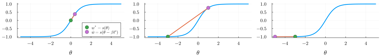
Figure 1: Adaptive straight-through estimation illustrated when $s$ is the $\tanh$ mapping. $\ell^{\prime}$ is the incoming back-propagated error signal. Left: $\theta\approx 0$. The finite difference slope $(\hat{w}-w^{*})/\beta$ matches the derivative of $\tanh$ very well. Middle: $\theta\ll 0$ and $\ell^{\prime}<0$. A nearly vanishing derivative of $\tanh$ is boosted and $\tanh$ becomes “leaky.” Right: $\theta\ll 0$ and $\ell^{\prime}>0$. No boosting of the gradient in this case. The case $\theta\gg 0$ is symmetrical.

In practice, one needs to address problem settings where the parameter dimension $d$ is very large (such as deep neural networks with many layers). However, addressing the binary constraints in the above program is a challenging task, which is due to the combinatorial and non-differentiable nature of the underlying optimization problem. In view of large training datasets, (stochastic) gradient-based methods to obtain minimizers of (1) are highly preferable. Various techniques have been proposed to address the above difficulties and convert (1) into a differentiable surrogate. The general approach is to introduce real-valued “latent” weights $\theta\in\mathbb{R}^{d}$, from which the effective weights $w=\operatorname{sgn}(\theta)$ are generated via the sign function (or a differentiable surrogate thereof). One of the simplest and nevertheless highly successful algorithms to train BiNNs termed BinaryConnect [10] is based on straight-through estimators (STE), which ignore the sign mapping entirely when forming the gradient w.r.t. the latent weights $\theta$. Although this appears initially not justified, BinnaryConnect works surprisingly well and is still a valid baseline method for comparison. More recently, the flexibility in choosing the distance-like mapping leveraged in the mirror descent method [32] (and in particular the entropic descent algorithm [7]) provides some justification of BinaryConnect-like methods [3] (see also Sec. 3.2).

In this work, we propose a new framework for training binary neural networks. In particular, we first formulate the training problem shown in (1) as a bilevel optimization task, which is subsequently relaxed using an optimal value reformulation. Further, we propose a novel scheme to calculate meaningful gradient surrogates in order to update the network parameters. The resulting method strongly resembles BinaryConnect but leverages an adaptive variant of the straight-through gradient estimator: the sign function is conditionally replaced by a suitable linear but data-dependent mapping. Fig. 1 illustrates the underlying principle for the $\tanh$ mapping: depending on the incoming error signal, vanishing gradients induced by $\tanh$ are conditionally replaced by non-vanishing finite-difference surrogates. We finally point out that our proposed method can be cast as a mirror descent method using a data-dependent and varying distance-like mapping.

2 Related Work

The practical motivation for exploring weight quantization is to reduce the computational costs of deploying (and in some cases training) neural networks. This can be particularly attractive in the case of edge computing and IoT devices [9]. Even when retaining floating point precision for activations $z$, using binarized weights matrices $W$ means that the omnipresent product $Wz$ reduces to cheaper additions and subtractions of floating point values.

Already in the early 1990s, [15, 44] trained BiNNs using fully local learning rules with layerwise targets computed via node perturbations. In order to avoid the limited scalability of node perturbations, [39] instead employed a differentiable surrogate of the sign function for gradient computation. Recently the use of differentiable surrogates in the backwards pass has been coined the Backward Pass Differentiable Approximation (BPDA) in the context of adversarial attacks [5]. However, the same principle is at the core of many network quantization approaches, most notably the STE for gradient estimation.

Recent approaches have mainly focused on variations of the STE. A set of real valued (latent) weights are binarized when computing the forward pass, but during the backwards pass the identity mapping is used as its differentiable surrogate (which essentially makes the STE a special case of BPDA). The computed gradients are then used to update the latent weights. The STE was presented by Hinton (and acredited to Krizhevsky) in a video lecture in 2012 [21]. Subsequently it was employed for training networks with binary activations in [8], and to train networks with binary weights (and floating point activations) in the BinaryConnect (BC) model [10]. BinaryConnect also used heuristics such as clipping the latent weights and employing Batch Normalization [24] (including its use at the output layer) to improve the performance of STE based training. Further and recent analysis of the straight-through estimator is provided in [47], where its origin is traced back to early work on perceptrons Rosenblatt [37, 38]. The STE has also been applied to training fully binarized neural networks (e.g. [23]). Moreover, Rastegari et al. [36] employ the STE for training fully binarized as well as mixed precision networks, and achieve improved performance by introducing layer and channel-wise scaling factors. An interesting line of research has explored adapting the STE for variable bit-width quantization with learnable quantization step sizes in [14] and learnable bit width in [43]. [43] also introduces a regularization based method for constraining the learned bit-width to conform to a user-specified memory budget.

Subsequent approaches have focused on deriving similar but less heuristic learning algorithms for networks with binary weights. ProxQuant (PQ) [6], Proximal Mean-Field (PMF) [2], Mirror Descent (MD) [3] and Rotated Binary Neural Networks (RBNN) [28] formulate the task of training DNNs with binary weights as a constrained optimization problem and propose different conversion functions used for moving between real-valued latent weights and binarized weights. A common feature among these methods is that they belong to the class of homotopy methods by gradually annealing the conversion mapping. Qin et al [35] introduce a novel technique for minimizing the information loss (caused by binarization) in the forward pass, and also aims to address gradient error by employing a gradually annealed tanh function as a differentiable surrogate during the backwards pass along with a carefully chosen gradient clipping schedule. Similar to early research, [20] does not introduce latent real-valued weights, but rather updates the binary weights directly using a momentum based optimizer designed specifically for BiNNs. Several authors have approached the training of quantized neural networks via a variational approach [31, 41, 1, 29]. Among those, BayesBiNN [31] is particularly competitive: instead of optimizing over binary weights, the parameters of Bernoulli distributions are learned by employing both a Bayesian learning rule [26] and the Gumbel-softmax trick [25, 30] (therefore requiring an inverse temperature parameter to convert the concrete distribution to a Bernoulli one).

For additional surveys of weight quantization we refer to the review papers [17, 34] as well as section III of [12]. For a review of the efficacy of various ad-hoc techniques commonly employed for training BiNNs we refer to [4].

3 Background

After clarifying some mathematical notations we summarize the mirror descent method (and its use to train BiNNs) and the Prox-Quant approach in order to better establish similarities and differences with our proposed method later.

3.1 Notation

A constraint such as $w\in C$ is written as $\imath_{C}(w)$ in functional form. We use $\odot$ to denote element-wise multiplication and $\oslash$ for element-wise division. The derivative of a function $\ell$ at $w$ is written as $\ell^{\prime}(w)$. Many mappings will be piece-wise differentiable but continuous. Therefore, in those cases $\ell^{\prime}(w)$ is a suitable element in the sub- or super-derivative. We use an arrow over some variable names (especially $\vec{\beta}$) to emphasize that this is a vector and not a scalar. For the same reason we use e.g. $\vec{s}$ and $\vec{\operatorname{sgn}}$ to indicate the vectorized form of a scalar mapping $s$ (or $\operatorname{sgn}$) that is applied element-wise.

3.2 Mirror Descent

In short, mirror descent [32, 7] successively generates new iterates by minimizing a regularized first-order surrogate of the target objective. The most common quadratic regularizer (which leads to the gradient descent method) is replaced by a more general Bregmen divergence penalizing large deviations from the previous iterate. The main motivation is to accelerate convergence of first-order methods, but it can also yield very elegant methods such as the entropic descent algorithm, where the utilized Bregman divergence based on the (negated) Shannon entropy is identical to the KL divergence. The entropic descent method is very natural when optimizing unknowns constrained to remain in the probability simplex $\Delta$. The algorithm repeats updates of the form

$$w^{(t+1)} \leftarrow\arg\min_{w\in\Delta}w^{\top}\ell^{\prime}(w^{(t)})+\tfrac{1}{\eta}D_{KL}(w\|w^{(t)})$$ (3)

with the associated first-order optimality condition

$$w_{j}^{(t+1)}\propto w_{j}^{(t)}e^{-\eta\ell^{\prime}(w^{(t)})_{j}}.$$ (4)

Reparametrizing $w$ as $w=\sigma(\theta)$, where $\sigma$ is the soft-arg-max function, $\sigma(u)_{j}=e^{u_{j}}/\sum_{j^{\prime}}e^{u_{j^{\prime}}}$, yields

$$\theta^{(t+1)} \leftarrow\theta^{(t)}-\eta\ell^{\prime}(w^{(t)})=\theta^{(t)}-\eta\ell^{\prime}(\sigma(\theta^{(t)})).$$ (5)

Interestingly, mirror descent modifies the chain rule by bypassing the inner derivative, since the update is based on $\ell^{\prime}(\sigma(\theta^{(t)}))$ and not on $\frac{d}{d\theta}\ell(\sigma(\theta^{(t)}))$ as in regular gradient descent. Hence, mirror descent is one way to justify the straight-through estimator. The entropic descent algorithm is leveraged in [3] to train networks with binary (and also generally quantized) weights. The soft-arg-max function $\sigma$ is slowly modified towards a hard arg-max mapping in order to ultimately obtain strictly quantized weights.

3.3 ProxQuant

ProxQuant [6] is based on the observation that the straight-through gradient estimator is linked to proximal operators via the dual averaging method [45]. The proximal operator for a function $\phi$ is the solution of the following least-squares regularized optimization problem,

$$\text{prox}_{\lambda\phi}(\theta)=\arg\min\nolimits_{\theta^{\prime}}\lambda\phi(\theta^{\prime})+\tfrac{1}{2}\|\theta^{\prime}-\theta\|^{2},$$ (6)

where $\lambda>0$ controls the regularization strength. If $\phi$ is a convex and lower semi-continuous mapping, the minimizer of the r.h.s. is always unique and $\text{prox}_{\lambda\phi}$ is a proper function (and plays an crucial role in many convex optimization methods). ProxQuant uses a non-convex mappings for $\phi$, which is far more uncommon for proximal steps than the convex case (see e.g. [42] for another example). In order to train DNNs with binary weights, $\phi$ is chosen as W-shaped function,

$$\phi(\theta)=\sum\nolimits_{j=1}^{d}\min\left\{|\theta_{j}-1|,|\theta_{j}+1|\right\}.$$ (7)

$\phi$ has $2^{d}$ isolated global minima and is therefore not convex. Note that $\text{prox}_{\lambda\phi}(\theta)$ is uniquely defined as long as all elements in $\theta$ are non-zero. The network weights are updated according to

$$\theta^{(t+1)}\leftarrow\text{prox}_{\lambda^{(t)}\phi}\left(\theta^{(t)}-\eta\ell^{\prime}(\theta^{(t)})\right),$$ (8)

and the regularization weight $\lambda^{(t)}$ is increased via an annealing schedule, which makes ProxQuant an instance of homotopy methods: strictly quantized weights are only obtained for a sufficiently large value of $\lambda^{(t)}$.

4 Adaptive Straight-Through Estimator

In this section, we propose a new approach to tackle the optimization problem given in (1). Reformulating and relaxing an underlying bilevel minimization problem is at the core of the proposed method.

4.1 Bilevel Optimization Formulation

We start by rewriting the original problem (1) as the following bilevel minimization program,

$$\min\nolimits_{\theta,w}\ell(w^{*})\quad\text{s.t. }w^{*}=\arg\min\nolimits_{w}\mathcal{E}(w;\theta)$$ (9)

where $\mathcal{E}(w;\theta)$ can be any function that favors $w^{*}$ to be binary. Two classical choices for $\mathcal{E}$ are given by

$$\mathcal{E}_{\text{tanh}}(w;\theta) =-\tfrac{1}{\tau}\sum\nolimits_{j}H\left(\tfrac{1}{2}(1-w_{j})\right)-w^{\top}\theta$$ (10)

$$\mathcal{E}_{\text{hard-tanh}}(w;\theta) =\tfrac{1}{2\tau}\lVert w\rVert^{2}-w^{\top}\theta+\imath_{[-1,1]^{d}}(w),$$ (11)

where $H$ is the Shannon entropy of a Bernoulli random variable, $H(u)=u\log u+(1-u)\log(1-u)$. The minimizer $w^{*}$ for given $\theta$ is the $\tanh$ mapping in the case of $\mathcal{E}_{\text{tanh}}$, $w_{j}^{*}=\tanh(\theta_{j}/\tau)$, and the second option yields the hard-tanh mapping, $w_{j}^{*}=\Pi_{[-1,1]}(\theta_{j}/\tau)$. $\tau>0$ is a parameter steering how well these mappings approximate the sign function $\vec{\operatorname{sgn}}(\theta)$.

In order to apply a gradient-based learning method we require that $\mathcal{E}$ is differentiable w.r.t. $\theta$ for all $w$. In the above examples we have $\frac{\partial}{\partial\theta}\mathcal{E}(w;\theta)=-w$. It will be sufficient for our purposes to assume that $\mathcal{E}$ is of the form

$$\mathcal{E}(w;\theta)=-w^{\top}\theta+\mathcal{G}(w)$$ (12)

for a coercive function $\mathcal{G}$ bounded from below. That is, $w$ and $\theta$ only interact via their (separable) inner product. Further, it is sufficient to assume that $\mathcal{G}$ is fully separable, $\mathcal{G}(w)=\sum_{j}G(w_{j})$, since each latent weight $\theta_{j}$ can be mapped to its binarized surrogate $w_{j}$ independently (an underlying assumption in the majority of works but explicitly deviated from in [18]). Thus, the general form for $\mathcal{E}$ assumed in the following is given by

$$\mathcal{E}(w;\theta)=\sum\nolimits_{j}\big{(}G(w_{j})-w_{j}\theta_{j}\big{)}.$$ (13)

Therefore in this setting the solution $w^{*}=(w_{1}^{*},\dotsc,w_{d}^{*})^{\top}$ is given element-wise,

$$w_{j}^{*}=\arg\min\nolimits_{w_{j}}G(w_{j})-w_{j}\theta_{j}.$$ (14)

4.2 Relaxing by Optimal Value Reformulation

The optimal value reformulation (e.g. [33, 48]), which is a commonly used reformulation approach in bilevel optimization, allows us to rewrite the bilevel problem (9) as follows,

$$\min\nolimits_{\theta,w}\ell(w)\quad\text{s.t. }\mathcal{E}(w;\theta)\leq\min\nolimits_{w^{\prime}}\mathcal{E}(w^{\prime};\theta).$$ (15)

Observe that the $w^{*}$ in the outer objective of (9) was replaced by a new unknown $w$, while the difficult equality constraint in (9) has been replaced by a somewhat easier inequality constraint. Due to the separable nature of $\mathcal{E}$ in (13), it is advantageous to introduce an inequality constraint for each element $w_{j}$. Thus, we obtain

$$\min\nolimits_{\theta,w}\ell(w)\quad\text{s.t. }E(w_{j};\theta_{j})\leq\min\nolimits_{w_{j}^{\prime}}E(w_{j}^{\prime};\theta_{j}),$$ (16)

where $E$ (independent of $j$) is given as

$$E(w_{j};\theta_{j}):=G(w_{j})-w_{j}\theta_{j}.$$ (17)

This first step enables us to straightforwardly relax (16) by fixing positive Lagrange multipliers for the inequality constraints:

$$\min_{\theta,w}\ell(w)+\sum\nolimits_{j}\tfrac{1}{\beta_{j}}\big{(}E(w_{j};\theta_{j})-\min\nolimits_{w_{j}^{\prime}}E(w_{j}^{\prime};\theta_{j})\big{)}.$$ (18)

We parametrize the non-negative multipliers via $\beta_{j}^{-1}$ for $\beta_{j}>0$, which will be convenient in the following. Since we are interested in gradient-based methods, we replace the typically highly non-convex “loss” $\ell$ (which subsumes the target loss and the mapping induced by the network) by its linearization at $w^{*}$, $\ell(w^{*})+(w-w^{*})^{\top}\ell^{\prime}(w^{*})$. Recall that $w^{*}=\arg\min_{w}\mathcal{E}(w;\theta)$ is the effective weight used in the DNN and is ideally close to $\vec{\operatorname{sgn}}(\theta)$. Overall, we arrive at the following relaxed objective to train a network with binary weights:

$$\mathcal{L}(\theta) =\ell(w^{*})-(w^{*})^{\top}\ell^{\prime}(w^{*})$$

$$+\sum\nolimits_{j}\min_{w_{j}}\left\{w_{j}\ell^{\prime}_{j}(w^{*})+\tfrac{1}{\beta_{j}}E(w_{j};\theta_{j})\right\}$$

$$-\sum\nolimits_{j}\min_{w_{j}}\left\{\tfrac{1}{\beta_{j}}E(w_{j};\theta_{j})\right\},$$ (19)

The inner minimization problems have the solutions

$$w_{j}^{*} =\arg\min\nolimits_{w_{j}}E(w_{j};\theta_{j})\qquad\text{and}$$

$$\hat{w}_{j} :=\arg\min\nolimits_{w_{j}}\beta_{j}\ell^{\prime}_{j}(w^{*})w_{j}+E(w_{j};\theta_{j}).$$ (20)

$\hat{w}=(\hat{w}_{1},\dotsc,\hat{w}_{d})^{\top}$ is based on a perturbed objective that incorporates the local (first-order) behavior of the outer loss $\ell$. Both $w^{*}$ and $\hat{w}$ implicitly depend on the current value of $\theta$, and $\hat{w}$ depends on a chosen “step size” vector $\vec{\beta}:=(\beta_{j})_{j=1}^{d}$ with each $\beta_{j}>0$. If $\mathcal{E}(\cdot;\theta)$ is continuous at $w=w^{*}$, then $\lim_{\beta_{j}\to 0^{+}}\hat{w}_{j}=w_{j}^{*}$. Further, if $\mathcal{E}$ is of the form given in (12), then $\hat{w}$ is as easy to compute as $w^{*}$:

Proposition 1.

Let $\mathcal{E}(w;\theta)=G(w)-w^{\top}\theta$ and $w^{*}=\arg\min_{w}\mathcal{E}(w;\theta)$ be explicitly given as $w^{*}=\vec{s}(\theta)$. Then

$$\hat{w}=\vec{s}\big{(}\theta-\vec{\beta}\odot\ell^{\prime}(w^{*})\big{)}.$$ (21)

Proof.

We simply absorb the linear perturbation term into $\theta$, yielding $\tilde{\theta}:=\theta-\vec{\beta}\odot\ell^{\prime}(w^{*})$, and therefore $\hat{w}$ solves

$$\hat{w}=\arg\min\nolimits_{w}G(w)-w^{\top}\tilde{\theta}=\arg\min\nolimits_{w}\mathcal{E}(w;\tilde{\theta}).$$ (22)

Hence, $\hat{w}=\vec{s}(\tilde{\theta})=\vec{s}(\theta-\vec{\beta}\odot\ell^{\prime}(w^{*}))$ as claimed. ∎

All of the interesting choices $\mathcal{E}$ lead to efficient forward mappings $s$ (like the choices $\mathcal{E}_{\text{tanh}}$ and $\mathcal{E}_{\text{hard-tanh}}$ given earlier that resulted in tanh and hard tanh functions).

4.3 Updating the latent weights $\theta$

For a fixed choice of $\vec{\beta}=(\beta_{1},\dotsc,\beta_{d})^{\top}$ with $\beta_{j}>0$, the relaxed objective $\mathcal{L}(\theta)$ in (19) is a nested minimization instance with a “min-min-max” structure. In some cases it is possible to obtain a pure “min-min-min” instance via duality [49], but in practice this is not necessary. Let $\theta^{(t)}$ be the current solution at iteration $t$, then our employed local model to determine the new iterate $\theta^{(t+1)}$ is given by

$$Q(\theta;\theta^{(t)}) =\sum\nolimits_{j}\tfrac{1}{\beta_{j}}\big{(}E(\hat{w}_{j};\theta_{j})-E(w_{j}^{*};\theta_{j})\big{)}$$

$$+\tfrac{1}{2\eta}\lVert\theta-\theta^{(t)}\rVert^{2},$$ (23)

where $w^{*}=\vec{s}(\theta^{(t)})$ and $\hat{w}=\vec{s}(\theta^{(t)}-\vec{\beta}\odot\ell^{\prime}(w^{*}))$ are the effective weights and its perturbed instance, respectively, evaluated at $\theta^{(t)}$. The last term in $Q$ regularizes deviations from $\theta^{(t)}$, and $\eta$ plays the role of the learning rate. Minimizing $Q(\theta;\theta^{(t)})$ w.r.t. $\theta$ yields a gradient descent-like update,

$$\theta^{(t+1)} =\arg\min\nolimits_{\theta}Q(\theta;\theta^{(t)})$$

$$=\theta^{(t)}-\eta\big{(}w^{*}-\hat{w}\big{)}\oslash\vec{\beta}$$ (24)

for the assumed form of $\mathcal{E}$ in (12). Each element of $(w^{*}-\hat{w})\oslash\vec{\beta}$, i.e. $(w_{j}^{*}-\hat{w}_{j})/\beta_{j}$, corresponds to a finite difference approximation (using backward differences) of

$$-\tfrac{d}{d\beta_{j}}s\big{(}\theta^{(t)}_{j}-\beta_{j}\ell^{\prime}_{j}(w^{*})\big{)}\big{|}_{\beta_{j}=0^{+}}$$ (25)

with spacing parameter $h_{j}=\beta_{j}\ell^{\prime}_{j}(w^{*})$. If $s$ is at least one-sided differentiable, then it can be shown that these finite differences converge to a derivative given by the chain rule when $\beta_{j}\to 0^{+}$ [48],

$$\tfrac{1}{\beta_{j}}\big{(}w_{j}^{*} -\hat{w}_{j}\big{)}\stackrel{{\scriptstyle\beta_{j}\to 0^{+}}}{{\to}}-\tfrac{d}{d\beta}s(\theta^{(t)}_{j}-\beta_{j}\ell^{\prime}_{j}(w^{*}))\big{|}_{\beta_{j}=0^{+}}$$

$$=\ell_{j}^{\prime}(s(\theta^{(t)}_{j}))s^{\prime}(\theta^{(t)}_{j})=\tfrac{d}{d\theta_{j}}\ell(s(\theta^{(t)})).$$ (26)

For non-infintesimal $\beta_{j}>0$ the finite difference slope $(w_{j}^{*}-\hat{w}_{j})/\beta_{j}$ corresponds to a perturbed chain rule,

$$\tfrac{1}{\beta_{j}}\big{(}w^{*}_{j}-\hat{w}_{j}\big{)}=\ell^{\prime}_{j}(w^{*})s^{\prime}\big{(}\theta_{j}^{(t)}-\gamma_{j}\ell^{\prime}_{j}(w^{*})\big{)}$$ (27)

(recall that $w^{*}=s(\theta^{(t)})$), where the inner derivative is evaluated at a perturbed argument $\theta^{(t)}-\vec{\gamma}\odot\ell^{\prime}(w^{*})$ for a $\vec{\gamma}\in[0,\vec{\beta}]$. This is a consequence of the mean value theorem. Moreover, if each $\beta_{j}$ is a stationary point of the mapping

$$\beta\mapsto\tfrac{1}{\beta}\big{(}w_{j}^{*}-\hat{w}_{j}\big{)}=\tfrac{1}{\beta}\big{(}w_{j}^{*}-s(\theta_{j}^{(t)}-\beta\ell^{\prime}_{j}(w^{*}))\big{)},$$ (28)

then by using the quotient rule it is easy to see that $\vec{\gamma}=\vec{\beta}$, and therefore

$$\tfrac{1}{\beta_{j}}\big{(}w_{j}^{*}-\hat{w}_{j}\big{)}=\ell_{j}^{\prime}(w^{*})s^{\prime}\big{(}\theta^{(t)}_{j}-\beta_{j}\ell^{\prime}_{j}(w^{*})\big{)}.$$ (29)

Additionally, the relation in (27) can be interpreted as a particular instance of mirror descent (recall Sec. 3.2) as shown in the appendix. Overall, the above means that we can relatively freely select where $s^{\prime}$ is actually evaluated. Since $s$ is naturally a “squashing” function mapping $\mathbb{R}$ to the bounded interval $[-1,1]$, gradient-based training using $s^{\prime}$ usually suffers from the vanishing gradient problem. Using the relaxed reformulation for bilevel programs allows us to select $\beta_{j}$ to obtain a desired descent direction as it will be described in Section 4.5.

The resulting gradient-based training method is summarized in Alg. 1. The algorithm is stated as full batch method, but the extension to stochastic variants working with mini-batches drawn from $p_{\text{data}}$ is straightforward. In the following section we discuss our choice of $\mathcal{E}$ and how to select suitable spacing parameters $\vec{\beta}^{(t)}>0$ in each iteration. Since $\vec{\beta}^{(t)}$ is chosen adaptively based on the values of $\theta^{(t)}$ and $\ell^{\prime}(w^{*})$ and used to perturb the chain rule, we call the resulting algorithm the adaptive straight-through estimator (AdaSTE) training method.

1:  Initialize $\theta^{(0)}$, choose learning rates $\eta^{(t)}$, $t=1,\dotsc$

2:  for $t=1,\dotsc$ do

3:     $w^{*}\leftarrow\vec{s}(\theta^{(t)})$

4:     Run regular back-propagation to determine $\ell^{\prime}(w^{*})$

5:     Determine $\vec{\beta}^{(t)}$ using (39)

6:     $\hat{w}\leftarrow\vec{s}\big{(}\theta^{(t)}-\vec{\beta}^{(t)}\odot\ell^{\prime}(w^{*})\big{)}$

7:     $\theta^{(t+1)}\leftarrow\theta^{(t)}-\eta^{(t)}(w^{*}-\hat{w})\oslash\vec{\beta}^{(t)}$

8:  end for

Algorithm 1 AdaSTE training method.

4.4 Our choice for the inner objective $\cal E$

In this section we will specify our choice for $\mathcal{E}$ (and thus the mapping $\vec{s}:\theta\mapsto\arg\min_{w}\mathcal{E}(w;\theta)$). The straightforward options of $\mathcal{E}_{\text{tanh}}$ and $\mathcal{E}_{\text{hard-tanh}}$ (Section 4.1) suffer from the fact that the induced arg-min mappings coincide exactly with the sign function only when the hyper-parameter $\tau^{-1}\to\infty$. We are interested in an inner objective $\mathcal{E}$ that yields perfect quanitized mappings for finite-valued choices of hyper-parameters. Inspired by the double-well cost used in ProxQuant [6], we design $\mathcal{E}$ as follows,

$$\mathcal{E}(w;\theta) =\tfrac{1+\mu}{2}\lVert w\rVert^{2}-w^{\top}\theta-\mu(1\!+\!\alpha)\lVert w\rVert_{1}+\imath_{[-1,1]^{d}}(w),$$ (30)

where $\mu>0$ and $\alpha\in(0,1)$ are free parameters. Note that $\mathcal{E}$ is only piecewise convex in $w$ for fixed $\theta$, but it is fully separable in $w_{j}$ with

$$E(w_{j};\theta_{j})=\tfrac{1+\mu}{2}w_{j}^{2}-w_{j}\theta_{j}-\mu(1\!+\!\alpha)|w_{j}|+\imath_{[-1,1]}(w_{j}).$$ (31)

Via algebraic manipulations we find the following closed-form expression for $\hat{w}_{j}$ (where we abbreviate $\ell^{\prime}$ for $\ell^{\prime}(w^{*})$),

$$\hat{w}_{j} =\arg\min_{w_{j}}\beta_{j}\ell^{\prime}_{j}w_{j}+E(w_{j};\theta_{j})$$

$$=\Pi_{[-1,1]}\left(\frac{\tilde{\theta}_{j}+\mu(1+\alpha)\operatorname{sgn}(\tilde{\theta}_{j})}{1+\mu}\right),$$ (32)

with $\tilde{\theta}_{j}:=\theta_{j}-\beta_{j}\ell_{j}^{\prime}$. In other words, the forward mapping $\vec{s}:\theta\mapsto w^{*}=s(\theta)$ for our choice of $\mathcal{E}$ is given by

$$\vec{s}(\theta) =\Pi_{[-1,1]^{d}}\left(\frac{\theta+\mu(1+\alpha)\vec{\operatorname{sgn}}(\theta)}{1+\mu}\right).$$ (33)

The piece-wise linear graph of this mapping is illustrated in Fig. 2 for $\alpha=1/100$ and three different choices of $\mu$. Let $\alpha\in(0,1)$ be given, then $\vec{s}(\theta)$ attains only values in $\{-1,1\}^{d}$ even for finite $\mu$, since

$$\frac{|\theta_{j}|+\mu(1+\alpha)}{1+\mu}\geq 1\iff|\theta_{j}|+\mu(1+\alpha)\geq 1+\mu$$

$$\iff|\theta_{j}|+\alpha\mu\geq 1,$$ (34)

which implies that any $\theta_{j}$ is always mapped to +1 or -1 when $\mu\geq 1/\alpha$ (and the exact values of $\mu$ and $\alpha$ do not matter in this case). Consequently we have both the option to train with strictly binary weights from the beginning, or to train via a homotopy method by adjusting $\alpha$ or $\mu$. Both choices lead to competitive results with the homotopy-based method having a small advantage in some cases as demonstrated in Section 5.

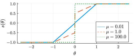
Figure 2: The graph of the mapping $w^{*}=s(\theta)$ given in (32) for $\alpha=1/100$ and three different values of $\mu$.

Implementation	CIFAR-10		CIFAR-100		TinyImageNet
	VGG-16	ResNet-18	VGG-16	ResNet-18	ResNet-18
Full-precision ($\dagger$)	93.33	94.84	71.50	76.31	58.35
BinaryConnect (*)	89.75$\pm$0.26	91.92$\pm$0.23	54.61$\pm$2.37	68.67$\pm$0.7	-
BinaryConnect ($\dagger$)	89.04	91.64	59.13	72.14	49.65
ProxQuant($\dagger$)	90.11	92.32	55.10	68.35	49.97
PMF($\dagger$)	91.40	93.24	64.71	71.56	51.52
MD-softmax ($\dagger$)	90.47	91.28	56.25	68.49	46.52
MD-softmax-s ($\dagger$)	91.30	93.28	63.97	72.18	51.81
MD-softmax-s (*)	83.69$\pm$0.33	91.56$\pm$0.14	48.23$\pm$0.55	68.35$\pm$0.96	-
MD-tanh ($\dagger$)	91.64	92.27	61.31	72.13	54.62
MD-tanh-s ($\dagger$)	91.53	93.18	61.69	72.18	52.32
MD-tanh-s (*)	90.22$\pm$0.24	91.41$\pm$0.11	60.14$\pm$0.58	66.38$\pm$0.26	-
BayesBiNN (*)	90.68$\pm$0.07	92.28$\pm$0.09	65.92$\pm$0.18	70.33$\pm$0.25	54.22
AdaSTE (no annealing) (*)	92.16$\pm$0.16	93.96$\pm$0.14	68.46$\pm$0.18	73.90$\pm$0.20	53.49
AdaSTE (with annealing) (*)	92.37$\pm$0.09	94.11$\pm$0.08	69.28$\pm$0.17	75.03$\pm$0.35	54.92

Table 1: Classification accuracy for different methods. (*) indicates that experiments have been run 5 times using different random seeds (except for TinyImageNet). ($\dagger$) indicates that results are obtained from the numbers reported by [3].

4.5 Adaptive choice for $\beta$

As indicated in Section 4.3, we can steer the modified chain rule by selecting $\beta_{j}>0$ appropriately in order to determine a suitable descent direction. Note that each element $\theta_{j}$ in the vector of parameters $\theta$ has its own value for $\beta_{j}$. Below we describe how $\beta_{j}$ is chosen when $\alpha$ and $\mu$ satisfy $\mu\alpha\geq 1$. In this setting we always have $w_{j}^{*}=\operatorname{sgn}(\theta_{j})\in\{-1,1\}$ and $\hat{w}_{j}=\vec{\operatorname{sgn}}(\theta_{j}-\beta_{j}\ell^{\prime}_{j}(w^{*}))\in\{-1,1\}$ (we ignore the theoretical possibility of $\theta_{j}=0$ or $\theta_{j}-\beta_{j}\ell_{j}^{\prime}(w^{*})=0$). Our aim is to select $\beta_{j}>0$ such that the slope induced by backward differences, $\frac{1}{\beta_{j}}(w_{j}^{*}-\hat{w}_{j})$, is as close to $\ell_{j}^{\prime}(w^{*})$ as possible. In the following we abbreviate $\ell^{\prime}(w^{*})$ to $\ell^{\prime}$.

Since $\operatorname{sgn}$ is an increasing step-function with derivative being zero almost everywhere, its finite difference approximation

$$\tfrac{1}{\beta_{j}}\big{(}w_{j}^{*}-\hat{w}_{j}\big{)}=\tfrac{1}{\beta_{j}}\big{(}\operatorname{sgn}(\theta_{j})-\operatorname{sgn}(\theta_{j}-\beta_{j}\ell^{\prime}_{j})\big{)}$$ (35)

lies either in the interval $[0,s_{\max}]$ or in $[-s_{\max},0]$ for a suitable $s_{\max}\geq 0$ (which is dependent on $\theta_{j}$ and $\ell^{\prime}_{j}$). In particular, if $\theta_{j}\ell^{\prime}_{j}\leq 0$, then $\operatorname{sgn}(\theta_{j})=\operatorname{sgn}(\theta_{j}-\beta_{j}\ell^{\prime}_{j})$ for all $\beta_{j}\geq 0$ and $s_{\max}=0$. On the other hand, if $\theta_{j}\ell^{\prime}_{j}>0$, then $\operatorname{sgn}(\theta_{j}-\beta_{j}\ell^{\prime}_{j})\neq\operatorname{sgn}(\theta_{j})$ for $\beta_{j}>\theta_{j}/\ell^{\prime}_{j}$ and therefore

$$\sup_{\beta_{j}>\theta_{j}/\ell^{\prime}_{j}}\frac{|w_{j}^{*}-\hat{w}_{j}|}{\beta_{j}}=\frac{2\ell^{\prime}_{j}}{\theta_{j}}.$$ (36)

If $\theta_{j}$ is close to 0, then the r.h.s. may grow arbitrarily large (reflecting the non-existence of the derivative of $\operatorname{sgn}$ at 0). Assuming that $(w_{j}^{*}-\hat{w}_{j})/\beta_{j}$ should maximally behave like a straight-through estimator (i.e. $|w_{j}^{*}-\hat{w}_{j}|/\beta_{j}\leq|\ell^{\prime}_{j}|$, which also can be seen as a form of gradient clipping), we choose

$$\beta_{j}=\tfrac{1}{|\ell^{\prime}_{j}|}\max\{2,|\theta_{j}|\}$$ (37)

in order to guarantee that

$$\tfrac{1}{\beta_{j}}|w_{j}^{*}-\hat{w}_{j}|\leq\tfrac{2}{\beta_{j}}\leq\tfrac{2|\ell^{\prime}_{j}|}{2}=|\ell^{\prime}_{j}|.$$ (38)

Overall, we obtain the following simple rule to assign each $\beta_{j}$ for given $\theta$ and $\ell^{\prime}$:

$$\beta_{j}\leftarrow\begin{cases}\tfrac{1}{|\ell^{\prime}_{j}|}\max\{2,|\theta_{j}|\}&\text{if }\theta_{j}\ell^{\prime}_{j}>0\\ 1&\text{otherwise.}\end{cases}$$ (39)

The choice of $\beta_{j}=1$ in the alternative case is arbitrary, since $(w_{j}^{*}-\hat{w}_{j})/\beta=0$ for all values $\beta>0$. Observe that the assignment of $\beta_{j}$ in (39) selectively converts $(w_{j}^{*}-\hat{w}_{j})/\beta_{j}$ into a scaled straight-through estimator whenever $\theta_{j}\ell^{\prime}_{j}>0$, otherwise the effective gradient used to update $\theta_{j}$ is zero (in agreement with the chain rule).

In the appendix we discuss the setting when $\mu\alpha<1$, which yields in certain cases different expressions for $\beta_{j}$. Nevertheless, we use (39) in all our experiments.

5 Experimental Results

In this section, we show several experimental results to validate the performance of our proposed method and compare it against existing algorithms that achieve state-of-the-art performance for our particular problem settings. As mentioned above, we only consider the training of networks with fully binarized weights and real-valued activations.

Following previous works [3, 6, 31], we use classification as the main task throughout our experiments. In particular, we evaluate the performance of the algorithms on the two network architectures: ResNet-18 and VGG16. The networks are trained and evaluated on the CIFAR10, CIFAR100 and TinyImageNet200 [27] datasets. We compare our algorithm against state-of-the-art approaches, including BinaryConnect (BC) [10], ProxQuant (PQ) [6], Proximal Mean-Field (PMF) [2], BayesBiNN [31], and several variants of Mirror Descent (MD) [3]. We employ the same standard data augmentations and normalization as employed by the methods we compare against (please refer to our appendix for more details about the experimental setup). Our method is implemented in Pytorch and is developed based on the software framework released by BayesBiNN’s authors (more details regarding our implementation can be found in the appendix).

5.1 Classification Accuracy

In Table 1, we report the best testing accuracy obtained by the considered methods. For PQ, PMF, the unstable versions of MD as well as for full-precision reference networks, we use the best results report in [3]. For BC, the stable variants of MD (i.e. MD-softmax-s and MD-tanh-s), we reproduce the results by running the source code released by the authors (using the default recommended hyper-parameters) for $5$ different random initializations, and reporting the mean and standard deviation obtained from these runs. The same strategy is also applied to BayesBiNN (hyper-parameters for BayesBiNN can be found in the appendix), except for the TinyImageNet dataset where we only report results for a single run (due to longer training time of TinyImageNet). We report the results for our method using two settings:

• Without annealing: we set $\alpha=0.01$ and fix $\mu=\frac{1}{\alpha}$ throughout training.

• With annealing: we also use $\alpha=0.01$ and set the initial value $\mu$ to $\mu^{(0)}=1.0$, then increase $\mu$ after each epoch by a factor of $\gamma$, i.e. $\mu^{(t)}\leftarrow\gamma\mu^{(t-1)}$. $\gamma$ is chosen such that $\mu$ reaches $1/\alpha$ after $\approx 200$ epochs.

The impact of the choice of $\mu$ on the shape of $\vec{s}(\theta)$ is illustrated in Fig. 2.

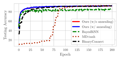
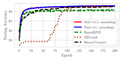
Figure 3: Testing accuracy achieved by the methods for the first 200 epochs with ResNet-18 (left) VGG16 (right) for CIFAR10 dataset (plots for CIFAR100 can be found in the appendix).

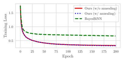
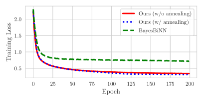
Figure 4: Training loss of the methods for the first 200 epochs with ResNet-18 (left) and VGG16 (right) on the CIFAR10 dataset (see appendix for plots of CIFAR100 dataset) .

Table 1 demonstrates that our proposed algorithm achieves state-of-the-art results. Note that we achieve highly competitive results even without annealing $\mu$ (although annealing improves the test accuracy slightly but consistently). Hence, we conclude that AdaSTE without annealing (and therefore no additional hyper-parameters) can be used as direct replacement for BinaryConnect. Note that we report all results after training for $500$ epochs. In the appendix, we will show that both BayesBiNN and AdaSTE yield even higher accuracy if the models are trained for higher number of epochs.

5.2 Evolution of Testing Accuracy and Training Losses

We further investigate the behavior of the algorithms during training. In particular, we are interested in the evolution of training losses and testing accuracy, since these quantities are—in addition to the achieved test accuracy—of practical interest.

In Fig. 3, we plot the testing accuracy obtained by our method in comparison with BC, MD (using the tanh mapping), and BayesBiNN for the first 200 epochs. For our method, we show the performance for both settings with and without annealing (as described earlier). To obtain the plots for MD and BayesBiNN, we use the code provided by the authors with the default recommended hyper parameters. For BC, we use the implementation provided by MD authors. As can be observed, AdaSTE quickly reaches very high test accuracy compared to other approaches. The MD-tanh approach (using the recommended annealing schedule from the authors [3]) only reaches satisfactory accuracy after approximately $100$ epochs. We also try starting MD-tanh with a larger annealing parameter (i.e. the $\beta$ hyper-parameter in [3]), but that yields very poor results (see the appendix for more details). AdaSTE, on the other hand, is quite insensitive to the annealing details, and yields competitive results even without annealing.

Fig. 4 depicts the training loss of our methods compared to BayesBiNN. We choose to compare AdaSTE against our main competitor, BayesBiNN, as we have full control of the source code to assure that both methods are initialized with the same starting points. As can be seen, our method quickly reduces the training loss, while BayesBiNN takes longer for the training loss to converge. Note that BayesBiNN leverages the reparametrization trick and relies therefore on weights sampled from respective distributions at training time. In that sense AdaSTE is a purely deterministic algorithm, and the only source of stochasticity is the sampled mini-batches. This might be a factor explaining AdaSTE’s faster reduction of the training loss.

6 Discussion and Conclusion

In this work we propose AdaSTE, an easy-to-implement replacement for the straight-through gradient estimator, and we demonstrate its benefits for training DNNs with strictly binary weights. One clear limitation in this work is, that we focus on the binary weight but real-valued activations scenario, which is a highly useful setting, but still prevents low-level implementations using only $\operatorname{xor}$ and bit count operations. Extending AdaSTE to binary activations seems straightforward, but will be more difficult to justify theoretically, and we expect training to be more challenging in practice. One obvious further shortcoming is our restriction to purely binary quantization levels, in particular to the set $\{+1,-1\}$. Generalizing the approach to arbitrary quantization levels can be done in several ways, e.g. by extending the W-shaped cost $E$ in (31) to more minima or by moving to higher dimensions (e.g. by modeling parameters in the probability simplex).

Since weight quantization is one option to regulate the Lipschitz property of a DNNs’ forward mapping (and also its expressive power), the impact of weight quantization [40, 13] (and more generally DNN model compression [16, 46]) on adversarial robustness has been recently explored. Hence, combining our adaptive straight-through gradient estimator with adversarial training is one direction of future work.

Appendix A A Mirror Descent Interpretation of AdaSTE

In this section we establish a connection between AdaSTE and mirror descent with a data-adaptive and varying metric. Since the update in AdaSTE is applied element-wise, we focus on the update of $\theta_{j}$ (a scalar) in the following. For brevity of notation we drop the subscript $j$.

We consider using a “partial” chain rule as follows. Let the target forward mapping be the composition of $s_{1}$ and $s_{2}$, i.e. $s=s_{2}\circ s_{1}$. Then the AdaSTE update step is abstractly given by

$$\theta^{(t+1)} \leftarrow\theta^{(t)}-\eta\ell^{\prime}(s_{2}(s_{1}(\theta^{(t)})))s_{2}^{\prime}(s_{1}(\theta^{(t)})).$$ (40)

Observe that only one step of the chain rule is applied on $\ell$ as $s_{1}^{\prime}$ is not used. We introduce an “intermediate” weight $u=s_{1}(\theta)$, and therefore $w=s_{2}(u)=s_{2}(s_{1}(\theta))=s(\theta)$. Expressing the above update step in $u$ yields

$$s_{1}^{-1}(u^{(t+1)}) \leftarrow s_{1}^{-1}(u^{(t)})-\eta\ell^{\prime}(s_{2}(u^{(t)}))s_{2}^{\prime}(u^{(t)}),$$ (41)

and identifying $s_{1}^{-1}$ with the mirror map $\nabla\Phi$ results eventually in

$$u^{(t+1)} =\arg\min_{u}\tfrac{1}{\eta}D_{\Phi}(u\|u^{(t)})+\ell^{\prime}(s_{2}(u^{(t)}))s_{2}^{\prime}(u^{(t)})$$

$$=\arg\min_{u}\tfrac{1}{\eta}D_{\Phi}(u\|u^{(t)})+\tfrac{d}{du}\ell(s_{2}(u))\big{|}_{u=u^{(t)}}.$$ (42)

Now the question is whether there exist mappings $s_{1}$ and $s_{2}$ such that

$$s_{2}(s_{1}(\theta))=s(\theta) s_{2}^{\prime}(u)=s^{\prime}(s_{1}^{-1}(u)-h),$$ (43)

where will be chosen as $h=\beta\ell^{\prime}$ in AdaSTE. The first relation yields

$$s_{1}(\theta)=s_{2}^{-1}(s(\theta))\;\text{ and }\;s_{1}^{-1}(u)=s^{-1}(s_{2}(u)).$$ (44)

Hence, the second condition above is equivalent to

$$s_{2}^{\prime}(u)=s^{\prime}(s_{1}^{-1}(u)-h)=s^{\prime}\big{(}s^{-1}(s_{2}(u))-h\big{)}.$$

By expressing this relation in terms of $\theta$ we obtain

$$s_{2}^{\prime}(s_{1}(\theta))=s^{\prime}(\theta-h)\iff s_{2}^{\prime}(s_{2}^{-1}(s(\theta)))=s^{\prime}(\theta-h)$$

$$\iff\frac{1}{(s_{2}^{-1})^{\prime}(s(\theta))}=s^{\prime}(\theta-h)$$

$$\iff(s_{2}^{-1})^{\prime}(w)=\frac{1}{s^{\prime}(s^{-1}(w)-h)}.$$

Consequently, $s_{2}^{-1}$ can be determined by solving

$$s_{2}^{-1}(w)=\int_{w_{0}}^{w}\frac{1}{s^{\prime}(s^{-1}(\omega)-h)}\,d\omega.$$ (45)

If $h=0$, then $s_{2}^{-1}=s^{-1}$ (and therefore $s_{1}=\mathrm{id}$) is a valid solution. For $h\neq 0$, there is sometimes a closed-form expression for $s_{2}^{-1}$. We consider $s=\tanh$, i.e.

$$s(\theta)=\frac{e^{\theta}-e^{-\theta}}{e^{\theta}+e^{-\theta}}=\frac{e^{2\theta}-1}{e^{2\theta}+1} s^{\prime}(\theta)=\frac{4e^{2\theta}}{(e^{2\theta}+1)^{2}}.$$ (46)

With this choice we obtain (via a computer algebra system)

$$(s_{2}^{-1})^{\prime}(w) =\frac{1}{s^{\prime}(s^{-1}(w)-h)}$$

$$=\frac{e^{-2h}\big{(}(e^{2h}-1)w-e^{2h}-1\big{)}^{2}}{4(1-w^{2})}$$

$$=\frac{\big{(}(e^{h}-e^{-h})w-e^{h}-e^{-h}\big{)}^{2}}{4(1-w^{2})}.$$ (47)

Now the following relation holds,

$$\int\frac{(aw+b)^{2}}{4(1-w^{2})}\,dw$$

$$\doteq\tfrac{1}{8}\left(-2a^{2}w-(a+b)^{2}\log(1-w)+(a-b)^{2}\log(1+w)\right).$$

Plugging in the values $a=e^{h}-e^{-h}$ and $b=-e^{h}-e^{-h}$ (and therefore $a+b=-2e^{-h}$ and $a-b=2e^{h}$) results in

$$s_{2}^{-1}(w)$$

$$=\tfrac{1}{8}\left(-2(e^{h}\!-\!e^{-h})^{2}w-4e^{-2h}\log(1\!-\!w)+4e^{2h}\log(1\!+\!w)\right)$$

$$=\tfrac{1}{2}\left(e^{2h}\log(1+w)-e^{-2h}\log(1-w)\right)$$

$$-\tfrac{1}{4}(e^{h}-e^{-h})^{2}w.$$ (48)

As expected, for $h=0$ we obtain $\tanh^{-1}$, and for $h\neq 0$ this mapping skews $\tanh^{-1}$. The important property is, that $s_{2}$ is strictly monotone since $s_{2}^{\prime}(s_{1}(\theta))=s^{\prime}(\theta-h)>0$. We can recover $s_{1}$ via $s_{1}(x)=s_{2}^{-1}(s(\theta))$, but that seems to be a non-interpretable expression in this case.

Appendix B AdaSTE: the case $\mu\alpha<1$

As in the previous section we focus on one scalar weight $\theta_{j}$/$w_{j}$ and omit the subscript $j$ in the following. We know that the actual weight $w$ is obtained via

$$w^{*} =\Pi_{[-1,1]}\left(\frac{\theta+\mu(1+\alpha)\operatorname{sgn}(\theta)}{1+\mu}\right)$$

$$\hat{w} =\Pi_{[-1,1]}\left(\frac{\tilde{\theta}+\mu(1+\alpha)\operatorname{sgn}(\tilde{\theta})}{1+\mu}\right),$$ (49)

where $\tilde{\theta}=\theta-\beta\ell^{\prime}$. We focus on $\theta<0$, since the case $\theta>0$ is symmetric. Hence,

$$w^{*}=\begin{cases}-1&\text{if }\theta\leq-1+\mu\alpha\\ \frac{\theta-\mu(1+\alpha)}{1+\mu}&\text{ if }\theta\in(-1+\mu\alpha,0)\end{cases}$$ (50)

and

$$\hat{w}=\begin{cases}-1&\text{if }\tilde{\theta}\leq-1+\mu\alpha\\ \frac{\tilde{\theta}-\mu(1+\alpha)}{1+\mu}&\text{ if }\tilde{\theta}\in(-1+\mu\alpha,0)\end{cases}.$$ (51)

We are now interested in values for $\beta>0$ maximizing $|\hat{w}-w^{*}|/\beta$. We assume that $\mu\alpha<1$, since the simpler setting $\mu\alpha\geq 1$ was discussed in the main text.

Case $\ell^{\prime}>0$:

We have $\tilde{\theta}=\theta-\beta\ell^{\prime}<\theta$ for all $\beta>0$. Since $\hat{w}$ will be clamped at $-1$ for sufficiently large $\beta>0$, the solution for $\beta$ satisfies

$$\theta-\beta\ell^{\prime}\in(-1+\mu\alpha,0).$$ (52)

If $\theta\leq-1+\mu\alpha$, then we have $w^{*}=\hat{w}=-1$ for all choices of $\beta$, and therefore $(\hat{w}-w^{*})/\beta=0$ regardless of $\beta$. Thus, we assume that $\theta>-1+\mu\alpha$ and therefore $w^{*}>-1$. For $\beta$ constrained as above, we have

$$\frac{\hat{w}-w^{*}}{\beta} =\frac{1}{\beta}\cdot\frac{\theta-\beta\ell^{\prime}-\mu(1+\alpha)-(\theta-\mu(1+\alpha))}{1+\mu}$$

$$=\frac{1}{\beta}\cdot\frac{\beta\ell^{\prime}}{1+\mu}=\frac{\ell^{\prime}}{1+\mu},$$

which is independent of the exact value of $\beta$ as long it is in the allowed range,

$$\beta\in\tfrac{1}{\ell^{\prime}}(\theta,\theta+1-\mu\alpha)\cap\mathbb{R}_{\geq 0}.$$ (53)

We can set $\beta$ as follows,

$$\beta=\min\left\{\beta_{\max},\frac{\theta+1-\mu\alpha}{\ell^{\prime}}\right\}$$

and the error signal is given by $(\hat{w}-w^{*})/\beta=\ell^{\prime}/(1+\mu)$.

Case $\ell^{\prime}<0$:

This means that $\tilde{\theta}>\theta$ for $\beta>0$. By inspecting the piecewise linear (and monotonically increasing) mapping $\theta\mapsto w^{*}$ we identify two relevant choices for $\beta$: $\beta_{1}$ as the smallest $\beta$ such that $\hat{w}$ is clamped at $+1$, and $\beta_{0}$ as the smallest $\beta$ such that $\hat{w}$ is positive. Note that $\tilde{\theta}$ is clamped at $+1$ whenever $\tilde{\theta}>1-\mu\alpha$. Therefore the defining constraints for $\beta_{1}$ and $\beta_{0}$ are given by

$$\theta-\beta_{1}\ell^{\prime}=1-\mu\alpha \theta-\beta_{0}\ell^{\prime}=0^{+},$$

i.e. $\beta_{1}=(\theta-1+\mu\alpha)/\ell^{\prime}$ and $\beta_{0}=\theta/\ell^{\prime}$ (and $\beta_{1}>\beta_{0}$ by construction). If $\tilde{\theta}=0^{+}$, then $\hat{w}=\mu(1+\alpha)/(1+\mu)$. Consequently,

$$\frac{\hat{w}_{1}-w^{*}}{\beta_{1}} =\frac{\ell^{\prime}}{\theta-1+\mu\alpha}\left(1-\max\left\{-1,\frac{\theta-\mu(1+\alpha)}{1+\mu}\right\}\right)$$

$$\frac{\hat{w}_{0}-w^{*}}{\beta_{0}} =\frac{\ell^{\prime}}{\theta}\left(\frac{\mu(1+\alpha)}{1+\mu}-\max\left\{-1,\frac{\theta-\mu(1+\alpha)}{1+\mu}\right\}\right).$$

If $\theta\leq-1+\mu\alpha$ such that $w^{*}=-1$, then these expressions simplify to

$$\frac{\hat{w}_{1}-w^{*}}{\beta_{1}} =\frac{2\ell^{\prime}}{\theta-1+\mu\alpha}>0$$

$$\frac{\hat{w}_{0}-w^{*}}{\beta_{0}} =\frac{\ell^{\prime}}{\theta}\cdot\frac{\mu+\mu\alpha+1+\mu}{1+\mu}=\frac{\ell^{\prime}(1+2\mu+\mu\alpha)}{(1+\mu)\theta}>0.$$

Now $(\hat{w}_{1}-w^{*})/\beta_{1}>(\hat{w}_{0}-w^{*})/\beta_{0}$ iff

$$\frac{2\ell^{\prime}}{\theta-1+\mu\alpha}>\frac{\ell^{\prime}(1+2\mu+\mu\alpha)}{(1+\mu)\theta}$$

$$\iff\frac{2}{\theta-1+\mu\alpha}<\frac{1+2\mu+\mu\alpha}{(1+\mu)\theta}$$

$$\iff 2(1+\mu)\theta<(\theta-1+\mu\alpha)(1+2\mu+\mu\alpha)$$

$$\iff(1-\mu\alpha)(\theta+1+2\mu+\mu\alpha)<0$$

$$\iff\theta<-1-2\mu-\mu\alpha.$$

Visual inspection shows that $\beta_{0}$ a good solution even when $\beta_{1}$ is the maximizer: $\beta_{0}$ does not maximize the slope $(\hat{w}-w^{*})/\beta$, but its slope is close to the maximal one.

If $\theta\in(-1+\mu\alpha,0)$, then $w^{*}=(\theta-\mu(1+\alpha))/(1+\mu)$ and therefore

$$\frac{\hat{w}_{1}-w^{*}}{\beta_{1}} =\frac{\ell^{\prime}}{\theta-1+\mu\alpha}\left(1-\frac{\theta-\mu(1+\alpha)}{1+\mu}\right)$$

$$=\frac{\ell^{\prime}}{\theta-1+\mu\alpha}\cdot\frac{1+\mu-\theta+\mu(1+\alpha)}{1+\mu}$$

$$\frac{\hat{w}_{0}-w^{*}}{\beta_{0}} =\frac{\ell^{\prime}}{\theta}\cdot\frac{\mu(1+\alpha)-\theta+\mu(1+\alpha)}{1+\mu}.$$

$(\hat{w}_{1}-w^{*})/\beta_{1}>(\hat{w}_{0}-w^{*})/\beta_{0}$ iff (after dividing both sides by $1+\mu>0$)

$$\frac{(1+2\mu+\mu\alpha-\theta)\ell^{\prime}}{\theta-1+\mu\alpha}>\frac{(2\mu(1+\alpha)-\theta)\ell^{\prime}}{\theta}$$

$$\iff\frac{1+2\mu+\mu\alpha-\theta}{\theta-1+\mu\alpha}<\frac{2\mu(1+\alpha)-\theta}{\theta}$$

$$\iff(1+2\mu+\mu\alpha-\theta)\theta<(2\mu(1+\alpha)-\theta)(\theta-1+\mu\alpha)$$

$$\iff 2\mu(1-\mu\alpha)(1+\alpha)<0$$

The l.h.s. is always positive under our assumptions, therefore $\beta_{0}=\theta/\ell^{\prime}$ is the maximizer in this case.

Appendix C Imagenette Results and Mixup

In order to further justify if our model also works well on images at higher resolution, we conduct the same experiment on Imagenette dataset [22] which are sampled from Imagenet [11] without being downsampled and consists of 9469 training images and 3925 validation images. Besides, we also notice that mixup [19], a proven effective training trick, is also helpful in further boosting the classification accuracy. As can be seen in Table 2, it is quite obvious that our AdaSTE consistenly outperforms BayesBiNN on both TinyImageNet and Imagenette datasets with and without mixup.

	TinyImageNet ResNet-18	Imagenette ResNet-18
BayesBiNN	54.22	78.19
BayesBinn (mixup)	55.84	79.59
AdaSTE	54.92	79.66
AdaSTE mixup)	56.11	80.91

Table 2: Classification accuracy for different methods on Tiny Imagenet and Imagenette: Annealing is applied to our model with and without mixup

Appendix D Implementation Details

We implemented our AdaSTE algorithm in PyTorch, which is developed based on the framework provided by BayesBiNN. In particular, we used SGD with momentum of $0.9$ for all experiments.

• For CIFAR-10 and CIFAR-100 datasets, we used batch size of $128$ with learning rate of $10^{-5}$.

• For TinyImageNet, the chosen batch size was $100$ with the learning rate of $10^{-6}$.

The experimental results for BayesBiNN were produced with the following hyper parameters:

• Batch size: $128$.

• Learning rate: $3\times 10^{-4}$.

• Momentum: $0.9$.

Appendix E CIFAR-100 Results

Similar to Fig. $3$ and Fig. $4$ in the main text, in Fig. 5 and Fig. 6, we also show the test accuracy and training loss versus number of epochs for the CIFAR-100 dataset with ResNet-18 and VGG-16 architectures. The same conclusion can also be drawn, where AdaSTE can quickly achieve very good performance, while it takes longer for other methods to yield high accuracy. This emphasizes the advantage of our method compared to existing approaches.

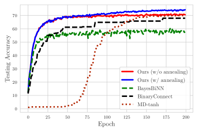
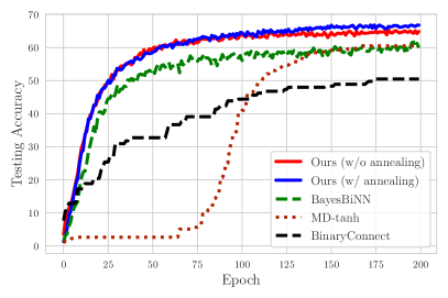
Figure 5: Testing accuracy achieved by the methods for the first 200 epochs with ResNet-18 (left) VGG16 (right) for CIFAR100 dataset.

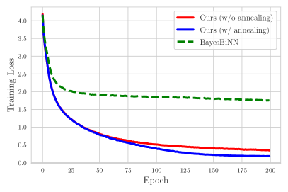
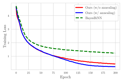
Figure 6: Training loss of the methods for the first 200 epochs with ResNet-18 (left) and VGG16 (right) on the CIFAR100 dataset.

Appendix F Training AdaSTE and BayesBiNN for a larger number of epochs

In Table $1$ in the main text, we report results obtained after training BayesBiNN and AdaSTE for $500$ epochs. In Fig. 7, we further show the progress of BayesBiNN and AdaSTE after training for $700$ epochs. As can be seen, the performance of both BayesBiNN and AdaSTE can still be improved, and BayesBiNN slowly approaches the performance of AdaSTE.

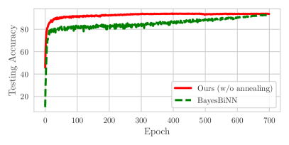
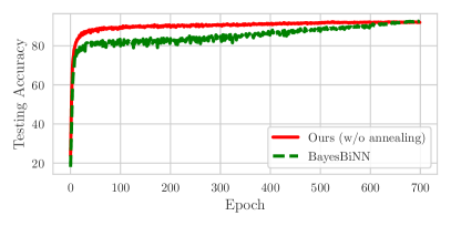
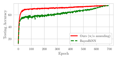
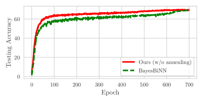
Figure 7: Testing accuracy achieved by the AdaSTE (no annealing) and BayesBiNN for 700 epochs. Top: CIFAR-10 with ResNet-18 (left) and VGG16 (right)

References

- [1] Jan Achterhold, Jan Mathias Koehler, Anke Schmeink, and Tim Genewein. Variational network quantization. In International Conference on Learning Representations, 2018.
- [2] Thalaiyasingam Ajanthan, Puneet K. Dokania, Richard Hartley, and Philip H. S. Torr. Proximal mean-field for neural network quantization. In Proceedings of the IEEE/CVF International Conference on Computer Vision (ICCV), October 2019.
- [3] Thalaiyasingam Ajanthan, Kartik Gupta, Philip Torr, Richard Hartley, and Puneet Dokania. Mirror descent view for neural network quantization. In Arindam Banerjee and Kenji Fukumizu, editors, Proceedings of The 24th International Conference on Artificial Intelligence and Statistics, volume 130 of Proceedings of Machine Learning Research, pages 2809–2817. PMLR, 13–15 Apr 2021.
- [4] Milad Alizadeh, Javier Fernández-Marqués, Nicholas D. Lane, and Yarin Gal. A systematic study of binary neural networks’ optimisation. In International Conference on Learning Representations, 2019.
- [5] Anish Athalye, Nicholas Carlini, and David Wagner. Obfuscated gradients give a false sense of security: Circumventing defenses to adversarial examples. In Jennifer Dy and Andreas Krause, editors, Proceedings of the 35th International Conference on Machine Learning, volume 80 of Proceedings of Machine Learning Research, pages 274–283. PMLR, 10–15 Jul 2018.
- [6] Yu Bai, Yu-Xiang Wang, and Edo Liberty. Proxquant: Quantized neural networks via proximal operators. In International Conference on Learning Representations, 2019.
- [7] Amir Beck and Marc Teboulle. Mirror descent and nonlinear projected subgradient methods for convex optimization. Operations Research Letters, 31(3):167–175, 2003.
- [8] Yoshua Bengio, Nicholas Léonard, and Aaron C. Courville. Estimating or propagating gradients through stochastic neurons for conditional computation. CoRR, abs/1308.3432, 2013.
- [9] Jiasi Chen and Xukan Ran. Deep learning with edge computing: A review. Proceedings of the IEEE, 107(8):1655–1674, 2019.
- [10] Matthieu Courbariaux, Yoshua Bengio, and Jean-Pierre David. BinaryConnect: Training Deep Neural Networks with binary weights during propagations. In C Cortes, N Lawrence, D Lee, M Sugiyama, and R Garnett, editors, Advances in Neural Information Processing Systems, volume 28. Curran Associates, Inc., 2015.
- [11] Jia Deng, Wei Dong, Richard Socher, Li-Jia Li, Kai Li, and Li Fei-Fei. Imagenet: A large-scale hierarchical image database. In CVPR, pages 248–255, 2009.
- [12] Lei Deng, Guoqi Li, Song Han, Luping Shi, and Yuan Xie. Model compression and hardware acceleration for neural networks: A comprehensive survey. Proceedings of the IEEE, 108(4):485–532, 2020.
- [13] Kirsty Duncan, Ekaterina Komendantskaya, Robert Stewart, and Michael Lones. Relative robustness of quantized neural networks against adversarial attacks. In 2020 International Joint Conference on Neural Networks (IJCNN), pages 1–8. IEEE, 2020.
- [14] Steven K. Esser, Jeffrey L. McKinstry, Deepika Bablani, Rathinakumar Appuswamy, and Dharmendra S. Modha. Learned step size quantization. In International Conference on Learning Representations, 2020.
- [15] Tal Grossman. The CHIR Algorithm for Feed Forward Networks with Binary Weights. In D Touretzky, editor, Advances in Neural Information Processing Systems, volume 2. Morgan-Kaufmann, 1990.
- [16] Shupeng Gui, Haotao N Wang, Haichuan Yang, Chen Yu, Zhangyang Wang, and Ji Liu. Model compression with adversarial robustness: A unified optimization framework. Advances in Neural Information Processing Systems, 32:1285–1296, 2019.
- [17] Yunhui Guo. A survey on methods and theories of quantized neural networks. CoRR, abs/1808.04752, 2018.
- [18] Kai Han, Yunhe Wang, Yixing Xu, Chunjing Xu, Enhua Wu, and Chang Xu. Training binary neural networks through learning with noisy supervision. In International Conference on Machine Learning, pages 4017–4026. PMLR, 2020.
- [19] Tong He, Zhi Zhang, Hang Zhang, Zhongyue Zhang, Junyuan Xie, and Mu Li. Bag of tricks for image classification with convolutional neural networks. In CVPR, pages 558–567, 2019.
- [20] Koen Helwegen, James Widdicombe, Lukas Geiger, Zechun Liu, Kwang-Ting Cheng, and Roeland Nusselder. Latent Weights Do Not Exist: Rethinking Binarized Neural Network Optimization. In H Wallach, H Larochelle, A Beygelzimer, F d´ Alché-Buc, E Fox, and R Garnett, editors, Advances in Neural Information Processing Systems, volume 32. Curran Associates, Inc., 2019.
- [21] G Hinton. Neural networks for machine learning, cousera video lectures, 2012.
- [22] Jeremy Howard and Sylvain Gugger. Fastai: a layered api for deep learning. Information, 11(2):108, 2020.
- [23] Itay Hubara, Matthieu Courbariaux, Daniel Soudry, Ran El-Yaniv, and Yoshua Bengio. Binarized Neural Networks. In D Lee, M Sugiyama, U Luxburg, I Guyon, and R Garnett, editors, Advances in Neural Information Processing Systems, volume 29. Curran Associates, Inc., 2016.
- [24] Sergey Ioffe and Christian Szegedy. Batch normalization: Accelerating deep network training by reducing internal covariate shift. In Francis Bach and David Blei, editors, Proceedings of the 32nd International Conference on Machine Learning, volume 37 of Proceedings of Machine Learning Research, pages 448–456, Lille, France, 07–09 Jul 2015. PMLR.
- [25] Eric Jang, Shixiang Gu, and Ben Poole. Categorical reparameterization with gumbel-softmax. arXiv preprint arXiv:1611.01144, 2016.
- [26] Mohammad Emtiyaz Khan and Håvard Rue. The bayesian learning rule, 2021.
- [27] Ya Le and Xuan Yang. Tiny imagenet visual recognition challenge. CS 231N, 7(7):3, 2015.
- [28] Mingbao Lin, Rongrong Ji, Zihan Xu, Baochang Zhang, Yan Wang, Yongjian Wu, Feiyue Huang, and Chia-Wen Lin. Rotated Binary Neural Network. In H Larochelle, M Ranzato, R Hadsell, M F Balcan, and H Lin, editors, Advances in Neural Information Processing Systems, volume 33, pages 7474–7485. Curran Associates, Inc., 2020.
- [29] Christos Louizos, Matthias Reisser, Tijmen Blankevoort, Efstratios Gavves, and Max Welling. Relaxed quantization for discretized neural networks. In International Conference on Learning Representations, 2019.
- [30] C Maddison, A Mnih, and Y Teh. The concrete distribution: A continuous relaxation of discrete random variables. In Proceedings of the international conference on learning Representations. International Conference on Learning Representations, 2017.
- [31] Xiangming Meng, Roman Bachmann, and Mohammad Emtiyaz Khan. Training binary neural networks using the Bayesian learning rule. In Hal Daumé III and Aarti Singh, editors, Proceedings of the 37th International Conference on Machine Learning, volume 119 of Proceedings of Machine Learning Research, pages 6852–6861. PMLR, 13–18 Jul 2020.
- [32] Arkadij Semenovi Nemirovskij and David Borisovich Yudin. Problem complexity and method efficiency in optimization. 1983.
- [33] Jií V Outrata. A note on the usage of nondifferentiable exact penalties in some special optimization problems. Kybernetika, 24(4):251–258, 1988.
- [34] Haotong Qin, Ruihao Gong, Xianglong Liu, Xiao Bai, Jingkuan Song, and Nicu Sebe. Binary neural networks: A survey. Pattern Recognition, 105:107281, Sep 2020.
- [35] Haotong Qin, Ruihao Gong, Xianglong Liu, Mingzhu Shen, Ziran Wei, Fengwei Yu, and Jingkuan Song. Forward and backward information retention for accurate binary neural networks. In Proceedings of the IEEE/CVF Conference on Computer Vision and Pattern Recognition (CVPR), June 2020.
- [36] Mohammad Rastegari, Vicente Ordonez, Joseph Redmon, and Ali Farhadi. XNOR-Net: ImageNet Classification Using Binary Convolutional Neural Networks. In Bastian Leibe, Jiri Matas, Nicu Sebe, and Max Welling, editors, Computer Vision – ECCV 2016, pages 525–542, Cham, 2016. Springer International Publishing.
- [37] F. Rosenblatt. The Perceptron, a Perceiving and Recognizing Automaton Project Para. Report: Cornell Aeronautical Laboratory. Cornell Aeronautical Laboratory, 1957.
- [38] F. Rosenblatt. Principles of Neurodynamics: Perceptrons and the Theory of Brain Mechanisms. Cornell Aeronautical Laboratory. Report no. VG-1196-G-8. Spartan Books, 1962.
- [39] D Saad and E Marom. Training Feed Forward Nets with Binary Weights Via a Modified CHIR Algorithm. Complex Systems, 4:573–586, 1990.
- [40] Chang Song, Elias Fallon, and Hai Li. Improving adversarial robustness in weight-quantized neural networks. arXiv preprint arXiv:2012.14965, 2020.
- [41] Daniel Soudry, Itay Hubara, and Ron Meir. Expectation backpropagation: Parameter-free training of multilayer neural networks with continuous or discrete weights. Advances in Neural Information Processing Systems, 2(January):963–971, 2014.
- [42] Evgeny Strekalovskiy and Daniel Cremers. Real-time minimization of the piecewise smooth mumford-shah functional. In European conference on computer vision, pages 127–141. Springer, 2014.
- [43] Stefan Uhlich, Lukas Mauch, Fabien Cardinaux, Kazuki Yoshiyama, Javier Alonso Garcia, Stephen Tiedemann, Thomas Kemp, and Akira Nakamura. Mixed precision dnns: All you need is a good parametrization. In International Conference on Learning Representations, 2020.
- [44] Santosh S. Venkatesh. Directed drift: A new linear threshold algorithm for learning binary weights on-line. Journal of Computer and System Sciences, 46(2):198–217, 1993.
- [45] Lin Xiao. Dual averaging methods for regularized stochastic learning and online optimization. Journal of Machine Learning Research, 11(88):2543–2596, 2010.
- [46] Shaokai Ye, Kaidi Xu, Sijia Liu, Hao Cheng, Jan-Henrik Lambrechts, Huan Zhang, Aojun Zhou, Kaisheng Ma, Yanzhi Wang, and Xue Lin. Adversarial robustness vs. model compression, or both? In Proceedings of the IEEE/CVF International Conference on Computer Vision, pages 111–120, 2019.
- [47] Penghang Yin, Jiancheng Lyu, Shuai Zhang, Stanley J. Osher, Yingyong Qi, and Jack Xin. Understanding straight-through estimator in training activation quantized neural nets. In International Conference on Learning Representations, 2019.
- [48] Christopher Zach. Bilevel programming and deep learning: A unifying view on inference learning methods. CoRR, abs/2105.07231, 2021.
- [49] Christopher Zach and Virginia Estellers. Contrastive learning for lifted networks. In British Machine Vision Conference, 2019.