Optimization of the $L^{1}$ norm of the solution of a Fisher-KPP equations in the small diffusivity regime

Abstract

We investigate in the present paper the maximization problem for the functional $F_{\mu}(m):=\int_{0}^{1}({\theta_{m,\mu}}-cm)$, where ${\theta_{m,\mu}}$ is the unique positive solution of $-\mu\theta^{\prime\prime}=\theta(m-\theta)$ in $(0,1)$, $\theta^{\prime}(0)=\theta^{\prime}(1)=0$, and $0\leq m\leq\kappa$. We assume $c\in(1,3)$. It is already known that the $BV$ norms of maximizers of this functional blow up when the diffusivity $\mu$ tends to $0$. Here, we first show that the maximizers are always $BV(0,1)$. Next, we completely characterize the limit of the maximas of this functional as $\mu\to 0$, and we show that one can construct a quasi-maximizer which is periodic, in a sense, and with a $BV$ norm behaving like $1/\sqrt{\mu}$. Lastly, we prove that along a subsequence $\mu_{k}\to 0$, any maximizer of $F_{\mu_{k}}$ is periodic, in a sense.

Key-words: logistic diffusive equation, heterogeneous Fisher-KPP, regularity and symmetry in optimization problems.

AMS classification. 34B15, 34C14, 49J15, 49K15

1 Introduction

The aim of this article is to describe the maximizers of

$$F_{\mu}(m):=\int_{0}^{1}({\theta_{m,\mu}}-cm)$$

where $\theta={\theta_{m,\mu}}$ is the unique positive solution of

$$-\mu\theta^{\prime\prime}=\theta(m-\theta)\quad\hbox{ in }(0,1),\quad\theta^{\prime}(0)=\theta^{\prime}(1)=0,$$ (1)

which is well-defined for all $m\in\mathcal{A}\backslash\{0\}$, where

$$\mathcal{A}:=\{m\in L^{\infty},\ 0\leq m\leq\kappa\hbox{ a.e. }[0,1]\}.$$

We consider the distribution of resources $m$ in the set of admissible functions $\mathcal{A}$.

1.1 Earlier works

This problem has first been raised by Lou [7] in a slightly different form, namely, he asked what were the maximizers of

$$G_{\mu}(m):=\int_{0}^{1}{\theta_{m,\mu}}$$

over the $m\in\mathcal{A}$, with $\int_{0}^{1}m=m_{0}$ prescribed. It is well-known that these two problems are dual in a sense. The first order optimality conditions were first derived in [2], where some numerics were also performed.

The author addressed this problem with Mazari and Privat in [10], and proved that only the two crenels $m=m_{cr,\ell}:=\kappa 1_{(0,\ell}$ and $m_{cr,\ell}(1-\cdot)$ are maximizers when $\mu$ is large enough. In particular, these maximizers are $BV(0,1)$ and bang-bang, that is, $m(x)\in\{0,\kappa\}$ for a.e. $x\in(0,1)$. Mazari [8] proved that the large diffusivity regime is related to the investigation of steady states for heterogeneous diffusive Lotka-Volterra competition systems.

In parallel, Nagahara and Yanagida [15] proved that the maximizers are bang-bang for all $\mu>0$, under the assumption that these maximizers are Riemann-measurable.

The regime $\mu\to 0$ was investigated by Mazari and Ruiz-Balet [12], who proved that the $BV$ norms of the maximizers necessarily tend to $+\infty$ as $\mu\to 0$, meaning that the maximizers oscillate very fastly between $0$ and $\kappa$ when $\mu$ is small. They performed some precise numerics describing such a behaviour, including multidimensional sets.

This property was improved by Mazari, Privat and the author [11], who proved that the $BV$ norms of the maximizers blow-up at least as $C/\sqrt{\mu}$ as $\mu\to 0$ for some constant $C>0$. They proved in the same paper that the maximizers are always bang-bang, regardless of any regularity large diffusivity assumption. The method used to derive this property is quite general and was used to derive bang-bang properties for a wide class of bilinear control problems by Mazari [9].

A discretized version of the problem, with discrete Laplacian, was investigated by Lou, Nagahara, and Yanagida in [14]. In that case, they managed to fully describe the maximizers when $\mu\to 0$. These maximizers are close to a periodic function. However, the connexion between this discrete problem and the continuous one is not clear in the small diffusivity regime $\mu\to 0$. Another discretized version of the equation, with equal diffusion rate between each patches, was investigated in [6].

Another related problem raised attention these last years: the maximization of the ratio $\int_{0}^{1}{\theta_{m,\mu}}/\int_{0}^{1}m$ under the constraint $m\geq 0$, $m\not\equiv 0$ on the growth rate. Bai, He and Li [1] proved that the supremum of this ratio is exactly $3$, and that a maximizing sequence $(m_{n})_{n}$ is the one concentrating to a Dirac mass at $x=1$. Inoue described the behaviour of ${\theta_{m,\mu}}$ along such a sequence in [4]. This ratio is not bounded anymore in multidimensional domains [3].

1.2 Statement of the results

Let now come back to the maximization of

$$F_{\mu}(m):=\int_{0}^{1}({\theta_{m,\mu}}-cm)$$

We assume in the present paper that $c\in(1,3)$.

If $c\geq 3$, then the unique maximizer of $F_{\mu}$ is $0$. Indeed, in that case, it has been proved in [1] that $\int_{0}^{1}{\theta_{m,\mu}}<3\int_{0}^{1}m$ for any non-constant $m$. Hence, $F_{\mu}(m)<0$ as soon as $m$ is non constant for $c\geq 3$. As ${\theta_{m,\mu}}\equiv m$ when $m$ is constant, one concludes that $0$ is the unique maximizer.

If $c\leq 0$, then clearly $m\equiv\kappa$ is the unique global maximizer.

Thus, only the case $c\in(0,1]$ remains relevant and is not covered by the present paper. We explain in Remark 2.4 the main obstacles in trying to extend the present method to $c\leq 1$.

We start with a regularity result on the maximizers.

Theorem 1

Assume that $c\in(1,3)$. Let $\overline{m}_{\mu}$ a maximizer of $F_{\mu}$ and assume that $\overline{m}_{\mu}\not\equiv 0$ and $\overline{m}_{\mu}\not\equiv\kappa$. Then the function $\theta_{\overline{m}_{\mu},\mu}^{\prime}$ admits a finite number of zeros, and $\overline{m}_{\mu}$ admits exactly one jump from $0$ to $\kappa$ between each of these zeros. In particular, $\overline{m}_{\mu}$ is $BV(0,1)$.

We will prove in Lemma 3.10, using a result of [1], that $\max_{\mathcal{A}(0,1)}F_{\mu}>0$ when $\mu$ is small enough. Hence, the hypotheses $\overline{m}_{\mu}\not\equiv 0$ and $\overline{m}_{\mu}\not\equiv\kappa$ are satisfied for $\mu$ small enough.

We now introduce a notion of functions of particular interest. Such functions appeared in the numerics performed in [12].

Definition 1.1

We say that a function $m\in L^{\infty}(0,1)$ is $k-$symmetric if there exist $l>0$, $k\in\mathbb{N}\backslash\{0\}$ and a function $m_{0}\in L^{\infty}(0,1)$, such that

$$m(x):=\left\{\begin{array}[]{lcll}m_{0}(y)&\hbox{ if }&x=\displaystyle\frac{2l}{k_{\mu}}+y,&\quad y\in[0,\frac{1}{k_{\mu}}),\\ m_{0}(1-y))&\hbox{ if }&x=\displaystyle\frac{2l+1}{k_{\mu}}+y,&\quad y\in[0,\frac{1}{k_{\mu}}),\\ \end{array}\right.$$

for all $l$ such that $l\leq l_{\mu}$, where we write $k=2l_{\mu}$ if $k$ is even, and $k=2l_{\mu}+1$ if $k$ is odd.

An example of a $k-$symmetric function is given at the bottom of Figure 1 below.

Let us denote for all $\ell\in[0,1]$ the crenel distribution as:

$$m_{cr,\ell}(x):=\left\{\begin{array}[]{rcl}\kappa&\hbox{ if }&x\in[0,\ell],\\ 0&\hbox{ if }&x\in(\ell,1].\\ \end{array}\right.$$

Theorem 2

Assume that $c\in(1,3)$. For all $\mu>0$, there exists $\hat{m}_{\mu}\in\mathcal{A}(0,1)$ such that $\|\hat{m}_{\mu}\|_{BV(0,1)}=k_{\mu}\simeq 1/\delta_{\mu}$ as $\mu\to 0$, $\hat{m}_{\mu}$ is $k_{\mu}$-symmetric with pattern $m_{cr,\ell}$ for some $\ell\in(0,1)$, and

$$\max_{m^{\prime}\in\mathcal{A}(0,1)}F_{\mu}(m^{\prime})-2\kappa\delta_{\mu}\leq F_{\mu}(\hat{m}_{\mu})\leq\max_{m^{\prime}\in\mathcal{A}(0,1)}F_{\mu}(m^{\prime}),$$

where

$$\overline{\mu}_{l}\leq\liminf_{\mu\to 0}\mu/\delta_{\mu}^{2}\leq\limsup_{\mu\to 0}\mu/\delta_{\mu}^{2}\leq\overline{\mu}_{l}$$

and $\overline{\mu}_{l}$ and $\overline{\mu}_{r}$ are positive constants given by Proposition 3.8.

Remark 1.2

We leave as an open problem the conjecture that $\overline{\mu}_{l}=\overline{\mu}_{r}$, that is, that $G$ admits a unique maximizer. This would imply the convergence of $\mu/\delta_{\mu}^{2}$ as $\mu\to 0$ to this unique maximizer. Liang and Lou [5] provided an example of growth rate $m$ for which $\mu\mapsto F_{\mu}(m)$ admits at least two maximas. However, the growth rates considered in the present paper are quite different from the one considered in [5], which was the perturbation of a constant function, and we thus still believe that $\overline{\mu}_{l}=\overline{\mu}_{r}$ here.

We do not know if the maximizers are always $k-$symmetric for $\mu$ small. In the numerics performed in [12], the maximizers did not always look like $k-$symmetric functions. However, when the diffusivity is well scaled, in a sense, we are able to prove that the maximizers are $k-$symmetric.

Theorem 3

Assume that $c\in(1,3)$. If one can write $\mu=\overline{\mu}/k^{2}$ for some $k\in\mathbb{N}\backslash\{0\}$ and $\overline{\mu}$ a maximizer of $\mu>0\mapsto G(\mu)$, then any maximizer $\overline{m}_{\mu}$ of $F_{\mu}^{(0,1)}$ is $K-$symmetric with pattern $m_{cr,\ell}$ for some $\ell>0$ and $K\in\mathbb{N}\backslash\{0\}$. Moreover, if $G$ admits a unique maximizer $\overline{\mu}$, then $K=k$.

2 $BV$ regularity of the maximizers

The aim of this section is to prove Theorem 1.

Consider the Hamiltonian

$$H(x,\theta,\theta^{\prime},p,p^{\prime},p^{0},m):=-\mu p^{\prime}\theta^{\prime}-p\theta(m-\theta)-(\theta-cm)$$

and the cost

$$C(m):=\int_{0}^{L}(-{\theta_{m,\mu}}+cm)=-F_{\mu}(m).$$

Let ${p_{m,\mu}}$ the unique solution of

$$-\mu p^{\prime\prime}-(m-2{\theta_{m,\mu}})p=1\quad\hbox{ in }(0,1),\quad p^{\prime}(0)=p^{\prime}(1)=0.$$ (2)

The Pontryagin maximum principle yields that a minimizer $\overline{m}_{\mu}$ of the cost (that is, a maximizer of $F_{\mu}$) satisfies

$$\overline{m}_{\mu}(x)=\left\{\begin{array}[]{lll}\kappa&\hbox{ if }&c>{p_{m,\mu}}(x){\theta_{m,\mu}}(x),\\ 0&\hbox{ if }&c<{p_{m,\mu}}(x){\theta_{m,\mu}}(x).\\ \end{array}\right.$$ (3)

We will now denote $m=\overline{m}_{\mu}$, $\theta={\theta_{m,\mu}}$ and $p={p_{m,\mu}}$ when there is no ambiguity in order to enlight the notations, and

$$\Phi:=\theta p.$$

The Hamiltonian $H$ is constant along the trajectories since the system is homogeneous (in the sense that the only heterogeneity is due to the control term $m$, see for instance [16], p. 96). Hence,

$$\mu p^{\prime}\theta^{\prime}+p\theta(m-\theta)+\theta-cm=cste\hbox{ in }(0,L).$$ (4)

Lemma 2.1

The set $\{\Phi=c\}$ has measure $0$.

Proof.

We just need a duality argument in order to apply Theorem I of [11].

Define $m_{0}:=\int_{0}^{1}\overline{m}_{\mu}$ and

$$\mathcal{A}_{m_{0}}:=\{m\in L^{\infty},\ 0\leq m\leq\kappa\hbox{ a.e. }[0,1],\ \int_{0}^{1}m=m_{0}\}.$$

Then

$$\int_{0}^{1}\theta_{\overline{m}_{\mu},\mu}\geq\int_{0}^{1}\theta_{m,\mu}\hbox{ for all }m\in\mathcal{A}_{m_{0}}.$$

Hence, the conclusion follows from Theorem I of [11]. $\Box$

Lemma 2.2

Assume that $c>1$. Let $0\leq a<1$ such that $\theta^{\prime}(a)=0$ and $\Phi(a)<c$. Then

$$b:=\min\{x\in(a,1],\ \theta^{\prime}(x)=0\}$$

is well-defined, $\theta^{\prime}>0$ in $(a,b)$, $\Phi$ only crosses $c$ once in $(a,b]$, and $\Phi(b)>c$.

Similarly, if $\Phi(a)>c$, then $b$ is still well-defined and $\theta^{\prime}<0$ in $(a,b]$, $\Phi$ only crosses $c$ once in $(a,b)$, and $\Phi(b)<c$.

Proof.

We just prove the first part, the other one being proved similarly. As $\Phi$ is continuous, we know that $\Phi<c$ in a right neighborhood $(a,a+\varepsilon)$ of $a$ and thus $m=0$ in $(a,a+\varepsilon)$. It follows that $\mu\theta^{\prime\prime}=\theta^{2}>0$ in $(a,a+\varepsilon)$ (since $\theta>0$ due to $m\not\equiv 0$) and thus, as $\theta^{\prime}(a)=0$, $\theta^{\prime}>0$ in $(a,a+\varepsilon)$. As $\theta^{\prime}(L)=0$, $b$ is well-defined and strictly larger than $a$.

Next, $\Phi(b)\leq c$ by contradiction. We know that if $\Phi\leq c$ in $(a,b)$, then as $\{\Phi=c\}$ has measure $0$ by Lemma 2.1, one would have $m=0$ a.e. and $\theta^{\prime\prime}>0$ a.e. in $(a,b)$, contradicting $\theta^{\prime}(b)=0$. Hence, there exists an interval $(x_{0},y_{0})\subset(a,b)$ such that $\Phi>c$, and thus $m=\kappa$, in this interval. Moreover, we could assume that $\Phi(y_{0})=p(y_{0})\theta(y_{0})=c$ and as $\Phi(a)=p(a)\theta(a)<c$ , one gets from (4):

$$\begin{array}[]{rcl}(1-c)\theta(a)&<&-p(a)\theta^{2}(a)+\theta(a)\\ &&\\ &=&\mu p^{\prime}(y_{0})\theta^{\prime}(y_{0})+c(m(y_{0})-\theta(y_{0}))+\theta(y_{0})-cm(y_{0})\\ &&\\ &=&\mu p^{\prime}(y_{0})\theta^{\prime}(y_{0})+(1-c)\theta(y_{0}).\\ \end{array}$$

As $\theta^{\prime}>0$ over $(a,b)$, one has $\theta(y_{0})>\theta(a)$ and thus, as $c>1$, one gets $p^{\prime}(y_{0})>0$. This implies $\Phi^{\prime}(y_{0})>0$, a contradiction since $\Phi(y_{0})=c$ and $\Phi>c$ in $(x_{0},y_{0})$. We have also proved that $\Phi$ only crosses $c$ once in $(a,b]$, otherwise, there exist $(x_{0},y_{0})$ as above and we could conclude similarly. $\Box$

Lemma 2.3

Assume that $c>1$. Then for all $a\in[0,1]$ such that $\theta^{\prime}(a)=0$, one has $\Phi(a)\neq c$.

Proof.

Assume that there exists $a\in[0,1]$ such that $\theta^{\prime}(a)=0$, and $\Phi(a)=c$. Assume by contradiction that there exists $\tilde{a}\in[0,1]$ such that $\theta^{\prime}(\tilde{a})=0$, and $\Phi(\tilde{a})\neq c$. If $\tilde{a}<a$, as any such $\tilde{a}$ is isolated by Lemma 2.2, one can assume that $\tilde{a}$ is the largest one satisfying this property. But then, either $\Phi(\tilde{a})>c$ and then $b:=\min\{x\in(a,L],\ \theta^{\prime}(x)=0\}$ satisfies $\Phi(b)<c$, which contradicts the definition of $\tilde{a}$ since $b$ is either $a$ or another point $x$ such that $\theta^{\prime}(x)=0$ and $\Phi(x)=c$. Similarly, if $\Phi(\tilde{a})<c$, then $\Phi(b)>c$ and we also reach a contradiction. If $\tilde{a}>a$, we reach a similar contradiction by assuming that $\tilde{a}$ is the smallest one satisfying this property and using again Lemma 2.2. Hence, we have proved by contradiction that for all $\tilde{a}$ such that $\theta^{\prime}(\tilde{a})=0$, one has $\Phi(\tilde{a})=c$. In particular $\Phi(0)=\Phi(1)=c$.

Next, assume that there exists an interval $(x_{0},y_{0})$ such that $\Phi>c$ on this interval. We could assume that $\Phi(x_{0})=\Phi(y_{0})=c$. The function $\theta^{\prime}$ does not vanish on $(x_{0},y_{0})$ since $\Phi>c$. Assume first that $\theta^{\prime}>0$ on $(x_{0},y_{0})$. We define $a=\max\{x\in[0,x_{0}],\theta^{\prime}(x)=0\}$ and $b=\min\{x\in[0,x_{0}],\theta^{\prime}(x)=0\}$. Then $\Phi(a)=\Phi(b)=0$ since $\theta^{\prime}(a)=\theta^{\prime}(b)=0$ and the same computations as in the proof of Lemma 2.2 yield

$$(1-c)\theta(a)=\mu p^{\prime}(y_{0})\theta^{\prime}(y_{0})+(1-c)\theta(y_{0}).$$

It follows that $p^{\prime}(y_{0})>0$ since $\theta(y_{0})>\theta(a)$ and $c>1$, a contradiction since $\Phi(y_{0})=c$ and $\Phi>c$ in $(x_{0},y_{0})$. If there exists an interval $(x_{0},y_{0})$ such that $\Phi<c$ on this interval, we reach a contradiction similarly.

Hence, we have proved by contradiction that if there exists $a\in[0,1]$ such that $\theta^{\prime}(a)=0$, and $\Phi(a)=c$, then $\Phi\equiv c$ on $(0,1)$. This is a contradiction with Lemma 2.1.

$\Box$

Proof of Theorem 1.

By Lemmas 2.2 and 2.3, we know that all the zeros of $\theta^{\prime}$ in $[0,1]$ are isolated. Hence, as $[0,1]$ is compact, $\theta^{\prime}$ only admits a finite number of zeros. Hence, by Lemma 2.2, $\Phi$ only crosses $c$ a finite number of times. By characterization (3), $m$ is $BV(0,1)$ and admits exactly one jumps between each zeros of $\theta^{\prime}$.

$\Box$

Remark 2.4

We do not know if Theorem 1 still holds when $0<c\leq 1$. The main difference when $c<1$ is that the constant function $m(x)=\kappa$ satisfies the first order optimality conditions. Indeed, in that case $\theta\equiv\kappa$, $p\equiv 1/\kappa$ and $\Phi\equiv 1\geq c$ almost everywhere. Hence, Lemmas 2.2 and 2.3 cannot hold for any functions $(\theta,p,m)$ satisfying $(\ref{eq:theta})$, $(\ref{eq:p})$, $(\ref{eq:bathtub})$ and $(\ref{eq:PMP})$. However, $m\equiv\kappa$ might only be a local maximizer of $F_{\mu}$, not a global one, and maybe Lemmas 2.2 and 2.3 still hold for global maximizers. We leave this possible extension as an open problem.

3 Existence of a quasi-maximizer

The aim of this section is to prove Theorem 2.

In all this section, we will specify the dependence of $F_{\mu}$ with respect to the interval considered. That is, we define

$$F_{\mu}^{(a,b)}(m):=\int_{a}^{b}(\theta-cm)$$

where $0\leq a<b\leq 1$ and $\theta$ is the unique positive solution of

$$-\mu\theta^{\prime\prime}=\theta(m-\theta)\quad\hbox{ in }(a,b),\quad\theta^{\prime}(a)=\theta^{\prime}(b)=0.$$ (5)

3.1 Construction of the quasi-maximizer $\hat{m}_{\mu}$

We consider $m=\overline{m}_{\mu}$ such that $F^{(0,1)}_{\mu}(m)=\max_{m^{\prime}\in\mathcal{A}(0,1)}F_{\mu}^{(0,1)}(m^{\prime})$. By Theorem 1, we denote by $(a_{i})_{1\leq i\leq N+1}$ the zeros of $\theta^{\prime}$, with $a_{0}=0$ and $a_{N+1}=1$, and we know that $m$ only jumps from $0$ to $\kappa$ once in each interval $(a_{i},a_{i+1})$. In other words,

$$\|m_{|(a_{i_{\mu}},a_{i_{\mu}+1})}\|_{BV(a_{i},a_{i+1})}=1.$$

Lemma 3.1

One has for all $i\geq 1$:

$$F^{(0,1)}_{\mu}(m)=\sum_{i=0}^{N}F^{(a_{i},a_{i+1})}_{\mu}(m).$$

Proof.

As $\theta^{\prime}(a_{i})=\theta^{\prime}(a_{i+1})=0$, the solution $\theta$ of (5), with $a=a_{i}$ and $b=a_{i+1}$ is just $\theta$ restricted to $(a_{i},a_{i+1})$ by uniqueness. Hence, $F^{(a_{i},a_{i+1})}_{\mu}(m)=\int_{a_{i}}^{a_{i+1}}(\theta-cm)$. The decomposition $F^{(0,1)}_{\mu}(m)=\sum_{i=1}^{N}F^{(a_{i},a_{i+1})}_{\mu}(m)$ follows.

$\Box$

We now define

$$A_{i}:=\frac{1}{a_{i+1}-a_{i}}F^{(a_{i},a_{i+1})}_{\mu}(m).$$

It follows from Lemma 3.1 that

$$F^{(0,1)}_{\mu}(m)=\sum_{i=0}^{N}(a_{i+1}-a_{i})A_{i}\leq\max_{0\leq i\leq N}A_{i}.$$

Let $i_{\mu}$ such that $\max_{0\leq i\leq N}A_{i}=A_{i_{\mu}}$. One obtains

$$F^{(0,1)}_{\mu}(m)\leq A_{i_{\mu}}\leq\frac{1}{a_{i_{\mu}+1}-a_{i_{\mu}}}\max_{m^{\prime}\in\mathcal{A}(a_{i_{\mu}},a_{i_{\mu}+1})}F_{\mu}^{(a_{i_{\mu}},a_{i_{\mu}+1})}(m^{\prime}).$$

Let

$$1=k_{\mu}(a_{i_{\mu}+1}-a_{i_{\mu}})+r_{\mu},\quad\hbox{ with }\quad 0\leq r_{\mu}<a_{i_{\mu}+1}-a_{i_{\mu}}.$$

We now construct a $k_{\mu}-$symmetric function $m_{|(a_{i_{\mu}},a_{i_{\mu}+1})}$ to $(0,1)$ by symmetrization and dilation. Namely, we define $\delta_{\mu}:=a_{i_{\mu}+1}-a_{i_{\mu}}$ and

$$\hat{m}_{\mu}(x):=\left\{\begin{array}[]{lcll}m\big{(}\sigma_{\mu}y+a_{i_{\mu}}\big{)}&\hbox{ if }&x=2l\frac{\delta_{\mu}}{\sigma_{\mu}}+y,&\quad y\in[0,\frac{\delta_{\mu}}{\sigma_{\mu}}),\\ m\big{(}a_{i_{\mu}+1}-\sigma_{\mu}y\big{)}&\hbox{ if }&x=(2l+1)\frac{\delta_{\mu}}{\sigma_{\mu}}+y,&\quad y\in[0,\frac{\delta_{\mu}}{\sigma_{\mu}}),\\ \end{array}\right.$$

for all $l$ such that $l\leq l_{\mu}$, where we write $k_{\mu}=2l_{\mu}$ if $k_{\mu}$ is even, and $k_{\mu}=2l_{\mu}+1$ if $k_{\mu}$ is odd, and where $\sigma_{\mu}:=k_{\mu}\delta_{\mu}=1-r_{\mu}$. This construction is described in Figure 1.

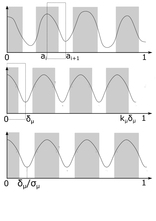
Figure 1: Construction of $\hat{m}_{\mu}$. First step: select the interval $(a_{i},a_{i+1})$ maximizing $A_{i}$. Second step: repeat periodically this pattern. Third step: stretch it so that it ends at $x=1$.

Lemma 3.2

One has for all $\lambda>0$, $\tilde{m}\in\mathcal{A}(0,1)$:

$$F_{\mu}^{(0,1)}(\tilde{m})=\lambda F_{\frac{\mu}{\lambda^{2}}}^{(0,1/\lambda)}\big{(}\tilde{m}(\lambda\cdot)\big{)}.$$

Proof.

Let $\theta:=\theta_{\tilde{m},\mu}$ and $\theta_{\lambda}(x):=\theta(\lambda x)$. One has

$$-\frac{\mu}{\lambda^{2}}\Delta\theta_{\lambda}(x)=\theta(\lambda x)\big{(}\tilde{m}(\lambda x)-\theta(\lambda x)\big{)}=\theta_{\lambda}(x)\big{(}\tilde{m}(\lambda x)-\theta_{\lambda}(x)\big{)}\hbox{ on }(0,1/\lambda).$$

Hence,

$$F_{\frac{\mu}{\lambda^{2}}}^{(0,1/\lambda)}\big{(}\tilde{m}(\lambda\cdot)\big{)}=\int_{0}^{1/\lambda}(\theta_{\lambda}-c\tilde{m}(\lambda\cdot))=\frac{1}{\lambda}\int_{0}^{1}(\theta-c\tilde{m})=\frac{1}{\lambda}F^{(0,1)}_{\mu}(\tilde{m}).$$

$\Box$

Lemma 3.3

Assume that $\tilde{m}\in\mathcal{A}(0,1)$ is a $k-$symmetric function with pattern $\tilde{m}_{0}$. Then for all $\mu>0$,

$$F_{\mu}^{(0,1)}(\tilde{m})=F_{k^{2}\mu}(\tilde{m}_{0}).$$

Proof.

Clearly, $F_{\mu}^{(0,1)}(\tilde{m})=\sum_{i=0}^{k-1}F_{\mu}^{(\frac{i}{k},\frac{i+1}{k})}(\tilde{m})$. Moreover, by symmetry and definition of $\tilde{m}$, one has $F_{\mu}^{(\frac{i}{k},\frac{i+1}{k})}(\tilde{m})=F_{\mu}^{(0,\frac{1}{k})}(\tilde{m})$. Hence,

$$F_{\mu}^{(0,1)}(\tilde{m})=kF_{\mu}^{(0,\frac{1}{k})}(\tilde{m})=F_{k^{2}\mu}^{(0,1)}\big{(}\tilde{m}(\cdot/k)\big{)}=F_{k^{2}\mu}^{(0,1)}(\tilde{m}_{0})$$

by Lemma 3.2. $\Box$

Lemma 3.4

One has

$$F_{\mu}^{(0,1)}(\hat{m}_{\mu})=\frac{1}{a_{i_{\mu}+1}-a_{i_{\mu}}}F_{\mu(1-r_{\mu})^{2}}^{(a_{i_{\mu}},a_{i_{\mu}+1})}(m).$$

Proof.

Let $\tilde{m}(x):=\hat{m}_{\mu}(x/\sigma_{\mu})$. This is the function corresponding to the second step described in Figure 1. One has by Lemma 3.2:

$$\sigma_{\mu}F_{\mu}^{(0,1)}\big{(}\hat{m}_{\mu}\big{)}=F_{\mu\sigma_{\mu}^{2}}^{(0,\sigma_{\mu})}(\tilde{m})=\sum_{j=0}^{k_{\mu}-1}F_{\mu\sigma_{\mu}^{2}}^{(j\delta_{\mu},(j+1)\delta_{\mu})}(\tilde{m}).$$

Next, it is clear that for all $j$, $F_{\mu\sigma_{\mu}^{2}}^{(j\delta_{\mu},(j+1)\delta_{\mu})}(\tilde{m})=F_{\mu\sigma_{\mu}^{2}}^{(a_{i_{\mu}},a_{i_{\mu}+1})}(m)$ by symmetry and definition of $\hat{m}_{\mu}$. Hence,

$$\sigma_{\mu}F_{\mu}^{(0,1)}\big{(}\hat{m}_{\mu}\big{)}=k_{\mu}F_{\mu\sigma_{\mu}^{2}}^{(a_{i_{\mu}},a_{i_{\mu}+1})}(m)$$

and the conclusion follows from $\sigma_{\mu}=k_{\mu}\delta_{\mu}=1-r_{\mu}$. $\Box$

Lemma 3.5

For all $\tilde{m}\in\mathcal{A}(0,1)$, $\mu\mapsto F_{\mu}(\tilde{m})$ is of class $\mathcal{C}^{1}$ and

$$\partial_{\mu}F_{\mu}(\tilde{m})\leq\kappa/\mu.$$

Proof.

The regularity follows from classical arguments and one has $\partial_{\mu}F_{\mu}(\tilde{m})=\int_{0}^{1}\dot{\theta}$, where $\dot{\theta}$ is the unique solution of

$$-\mu\dot{\theta}^{\prime\prime}-(\tilde{m}-2\theta_{\tilde{m},\mu})\dot{\theta}=\theta_{\tilde{m},\mu}^{\prime\prime}\hbox{ in }(0,1),\quad\dot{\theta}^{\prime}(0)=\dot{\theta}^{\prime}(1)=0.$$

Straightforward computations yield that $\theta_{\tilde{m},\mu}/\mu$ is a supersolution of this equation and thus the weak maximum principle yields

$$\dot{\theta}\leq\theta_{\tilde{m},\mu}/\mu\leq\kappa/\mu,$$

from which the conclusion follows. $\Box$

Lemma 3.6

For all $\tilde{m}\in\mathcal{A}(0,1)$, $\mu>0$ and $r\in(0,1)$, one has

$$F_{\mu(1-r)^{2}}^{(0,1)}(\tilde{m})-F_{\mu}^{(0,1)}(\tilde{m})\geq-2\kappa r.$$

Proof.

There exists $\xi\in\big{(}\mu(1-r)^{2},\mu\big{)}$ such that

$$F_{\mu(1-r)^{2}}^{(0,1)}(\tilde{m})-F_{\mu}^{(0,1)}(\tilde{m})=\partial_{\mu}F_{\xi}^{(0,1)}(\tilde{m})\big{(}\mu(1-r)^{2}-\mu\big{)}\geq-\kappa\big{(}1-(1-r)^{2}\big{)}\geq-2\kappa r.$$

$\Box$

Gathering all the previous estimates, we have thus obtained the following intermediate result.

Proposition 3.7

There exists $\hat{m}_{\mu}\in\mathcal{A}(0,1)$ such that $\|\hat{m}_{\mu}\|_{BV(0,1)}=k_{\mu}$ and

$$\max_{m^{\prime}\in\mathcal{A}(0,1)}F_{\mu}(m)-2\kappa\delta_{\mu}\leq F_{\mu}(\hat{m}_{\mu})\leq\max_{m^{\prime}\in\mathcal{A}(0,1)}F_{\mu}(m).$$

3.2 Estimates on $\mu/\delta_{\mu}^{2}$

The aim of this section is to prove Proposition 3.8, which, combined with Proposition 3.7, ends the proof of Theorem 2.

Proposition 3.8

Consider a sequence $(\mu_{k})_{k}$ such that $\lim_{k\to+\infty}\mu_{k}=0$, $(\mu_{k}/\delta_{\mu_{k}}^{2})_{k}$ converges to $\mu_{0}\geq 0$, and $(\ell_{\mu_{k}})_{k}$ converges to $\ell_{0}$ as $k\to+\infty$. Then

$$F_{\mu_{0}}^{(0,1)}(m_{cr,\ell_{0}})\geq F_{\mu}^{(0,1)}(m_{cr,\ell})\quad\hbox{ for all }\ell\in[0,1],\mu>0.$$

In particular,

$$\overline{\mu}_{l}\leq\liminf_{\mu\to 0}\mu/\delta_{\mu}^{2}\leq\limsup_{\mu\to 0}\mu/\delta_{\mu}^{2}\leq\overline{\mu}_{l}$$

where, if we let $G(\mu):=\sup_{\ell\in[0,1]}F_{\mu}^{(0,1)}(m_{cr,\ell})$, one defines

$$\overline{\mu}_{l}=\min\{\mu>0,G(\mu)=\sup_{\mu^{\prime}>0}G(\mu^{\prime})\}\hbox{ and }\overline{\mu}_{r}=\max\{\mu>0,G(\mu)=\sup_{\mu^{\prime}>0}G(\mu^{\prime})\},$$

and these two quantities are positive and finite.

Figure 2: An illustration of the definitions of $\overline{\mu}_{l}$ and $\overline{\mu}_{r}$.

Let first compare the supremum $F^{(0,1)}_{\mu}(m)$ with an appropriate function. Consider $\ell\in[0,1]$, $k\in\mathbb{N}\backslash\{0\}$ and $\tilde{m}(x)$ a $k-$symmetric function with pattern $m_{cr,\ell}$. Gathering all the previous inequalities and using Lemma 3.3, we have:

$$A_{i_{\mu}}=F^{(0,1)}_{\mu/\delta_{\mu^{2}}}(m_{cr,\ell_{\mu}})\geq F^{(0,1)}_{\mu}(m)\geq F^{(0,1)}_{\mu}(\tilde{m})=F^{(0,1)}_{\mu k^{2}}(m_{cr,\ell}).$$ (6)

We now need to make sure that $\mu/\delta_{\mu^{2}}$ is not too large nor too small.

Lemma 3.9

There exists a constant $C>0$ such that for all $m\in\mathcal{A}$ and $\mu>0$, one has

$$\big{\|}\theta_{m,\mu}-\int_{0}^{1}m\big{\|}_{L^{\infty}(0,1)}\leq C\kappa^{3/2}/\sqrt{\mu}.$$

Proof.

Multiplying the equation satisfied by ${\theta_{m,\mu}}$ by ${\theta_{m,\mu}}$ and integrating by parts, one gets

$$\mu\int_{0}^{1}({\theta_{m,\mu}}^{\prime})^{2}=\int_{0}^{1}{\theta_{m,\mu}}^{2}(m-{\theta_{m,\mu}})\leq\kappa^{3}.$$

It follows from the $(\infty,2)$ Poincaré inequality [13] that there exists a constant $C>0$ such that

$$\big{\|}{\theta_{m,\mu}}-\int_{0}^{1}{\theta_{m,\mu}}\big{\|}_{L^{\infty}(0,1)}\leq\frac{C\kappa^{3/2}}{6\sqrt{\mu}}.$$

On the other hand, integrating the equation satisfied by ${\theta_{m,\mu}}$, one gets

$$\int_{0}^{1}{\theta_{m,\mu}}m=\int_{0}^{1}{\theta_{m,\mu}}^{2}$$

and thus, writing ${\theta_{m,\mu}}=\int_{0}^{1}{\theta_{m,\mu}}+\eta$:

$$\int_{0}^{1}{\theta_{m,\mu}}\big{(}\int_{0}^{1}({\theta_{m,\mu}}-m)\big{)}=\int_{0}^{1}\eta m-2\int_{0}^{1}{\theta_{m,\mu}}\int_{0}^{1}\eta-\int_{0}^{1}\eta^{2}\leq\int_{0}^{1}\eta m-2\int_{0}^{1}{\theta_{m,\mu}}\int_{0}^{1}\eta.$$

As $\int_{0}^{1}{\theta_{m,\mu}}\geq\int_{0}^{1}m$, one gets

$$0\leq\int_{0}^{1}({\theta_{m,\mu}}-m)\leq\|\eta\|_{L^{\infty}(0,1)}+2\int_{0}^{1}|\eta|\leq C\kappa^{3/2}/(2\sqrt{\mu}),$$

from which the conclusion follows. $\Box$

Lemma 3.10

For all $c<3$, one has

$$\limsup_{\mu\to 0}\sup_{\ell\in[0,1]}F_{\mu}^{(0,1)}(m_{cr,\ell})=\sup_{\mu>0}\sup_{\ell\in[0,1]}F_{\mu}^{(0,1)}(m_{cr,\ell})>0.$$

Proof.

The identity between the $\limsup$ and the $\sup$ could be proved exactly as in [12].

Next, we consider the sequence $m_{cr,\varepsilon}$, that is

$$m_{cr,\varepsilon}(x):=\left\{\begin{array}[]{rcl}\kappa&\hbox{ if }&x\in[0,\varepsilon],\\ 0&\hbox{ if }&x\in(\varepsilon,1].\\ \end{array}\right.$$

It has been proved in [1] that

$$F_{\sqrt{\varepsilon}}^{(0,1)}(\frac{1}{\kappa\varepsilon}m_{cr,\varepsilon})\to 3\int_{0}^{1}\frac{m_{cr,\varepsilon}}{\kappa\varepsilon}\quad\hbox{ as }\varepsilon\to 0.$$

Hence, we could consider $c^{\prime}\in(c,3)$ and $\varepsilon$ small enough such that

$$F_{\sqrt{\varepsilon}}^{(0,1)}(\frac{1}{\kappa\varepsilon}m_{cr,\varepsilon})+c\geq 3-c^{\prime}+c,$$

where we have used $\int_{0}^{1}m_{cr,\varepsilon}=\kappa\varepsilon$. Next, one easily checks by considering $\theta_{B}:=B{\theta_{m,\mu}}$ that for all $\mu>0$, $B>0$ and $m\in L^{\infty}(0,1)$, $m\geq 0$, one has

$$F_{B\mu}^{(0,1)}(Bm)=BF_{\mu}^{(0,1)}(m).$$

Hence,

$$F_{\kappa\varepsilon^{3/2}}^{(0,1)}(m_{cr,\varepsilon})\geq(3-c^{\prime})\varepsilon\kappa>0,$$

which ends the proof. $\Box$

Lemma 3.11

There exists $M>0$ such that $1/M\leq\mu/\delta_{\mu}^{2}\leq M$ for all $\mu>0$.

Proof.

Assume first that there exists a sequence $(\mu_{j})_{j}$ such that $\lim_{j\to\infty}\mu_{j}/\delta_{\mu_{j}}^{2}=0$. We can assume, up to extraction, that there exists $\ell_{0}\in[0,1]$ such that $\lim_{j\to+\infty}\ell_{\mu_{j}}=\ell_{0}$. It has been proved in [12] that for all $M>0$, $\|{\theta_{m,\mu}}-m\|_{L^{1}(0,1)}\to 0$ as $\mu\to 0$ uniformly on function $m\in\mathcal{A}(0,1)$ such that $\|m\|_{BV(0,1)}\leq M$. In particular, as crenels have $BV-$norms equal to $1$, one has $\|\theta_{m_{cr,\ell},\mu}-m_{cr,\ell}\|_{L^{1}(0,1)}\to 0$ as $\mu\to 0$ uniformly with respect to $\ell\in[0,1]$.

We thus obtain

$$A_{i_{\mu_{j}}}=F^{(0,1)}_{\mu_{j}/\delta_{\mu_{j}^{2}}}(m_{cr,\ell_{\mu_{j}}})\to(1-c)\int_{0}^{1}m_{cr,\ell_{0}}=\kappa(1-c)\ell_{0}\leq 0\hbox{ as }j\to+\infty.$$

As

$$\lim_{j\to+\infty}A_{i_{\mu_{j}}}\geq\limsup_{j\to+\infty}F_{\mu_{j}}^{(0,1)}(\overline{m}_{\mu_{j}})=\limsup_{\mu\to 0}F_{\mu}^{(0,1)}(\overline{m}_{\mu})=\sup_{\mu>0}F_{\mu}^{(0,1)}(\overline{m}_{\mu})>0$$

by Lemma 3.10, one reaches a contradiction.

Next, if there exists a sequence $(\mu_{j})_{j}$ such that $\lim_{j\to\infty}\mu_{j}/\delta_{\mu_{j}}^{2}=+\infty$, then Lemma 3.9 yields

$$A_{i_{\mu_{j}}}=F^{(0,1)}_{\mu_{j}/\delta_{\mu_{j}^{2}}}(m_{cr,\ell_{\mu_{j}}})\simeq(1-c)\int_{0}^{1}m_{cr,\ell_{\mu_{j}}}=\kappa(1-c)\ell_{\mu_{j}}\leq 0\hbox{ as }j\to+\infty,$$

leading to a contradiction again. $\Box$

Proof of Proposition 3.8.

Let $(\mu_{j})_{j}$ such that $\mu_{j}\to 0$, $\mu_{j}/\delta_{\mu_{j}}^{2}\to\mu_{0}\in[1/M,M]$ and $\ell_{\mu_{j}}\to\ell_{0}$ as $j\to+\infty$.

Take $\mu>0$ and $\ell\in(0,1)$. There exists a sequence of integers $(k_{j})_{j}$ such that $1/\delta_{\mu_{j}}=k_{j}+r_{j}$, with $0\leq r_{j}<1$. Inequality (6) then yields

$$F^{(0,1)}_{\mu_{0}}(m_{cr,\ell_{0}})=\lim_{j\to+\infty}F^{(0,1)}_{\mu_{j}/\delta_{\mu_{j}^{2}}}(m_{cr,\ell_{\mu_{j}}})\geq\lim_{j\to+\infty}F^{(0,1)}_{\mu_{j}k_{j}^{2}}(m_{cr,\ell})=F^{(0,1)}_{\mu_{0}}(m_{cr,\ell})$$

since $\delta_{\mu_{j}}\to 0$.

Lastly, it follows from the same arguments as in the proof of Lemma 3.11 that $\overline{\mu}_{l}>0$ and $\overline{\mu}_{r}<\infty$.

$\Box$

4 The equality case

The aim of this section is to prove Theorem 3. We begin with a characterization of $k-$symmetric functions. We denote again $m=\overline{m}_{\mu}$, $\theta={\theta_{m,\mu}}$ and $p={p_{m,\mu}}$ when there is no ambiguity.

Lemma 4.1

Assume that there exists $a\in(0,1)$ such that $\theta^{\prime}(a)=0$ and $p^{\prime}(a)=0$. Then there exists $k\in\mathbb{N}$, $k\geq 1$, such that $m$ is $k-$symmetric.

Proof.

By using the change of variable $x^{\prime}:=1-x$ if necessary, we can always assume that $a\in(0,1/2]$. Consider the symmetrized function $m_{s}(x):=m(2a-x)$ if $x\in[a,2a]$, $m(x)$ if $x\in[0,a]$, and define similarly $\theta_{s}$, and $p_{s}$. These functions satisfy $(\ref{eq:theta})$ and $(\ref{eq:p})$ on $(0,2a)$.

We know that $\Phi(a)\neq c$ by Lemma 2.3. We can assume that $\Phi(a)>c$, the other case being treated similarly. Let

$$x_{0}:=\inf\{x\in(0,a),\Phi>c\hbox{ in }(x,a)\}\hbox{ and }y_{0}:=\inf\{x\in(a,2a),\Phi(x)>c\}.$$

By continuity of $\Phi$, $x_{0}<a<y_{0}$. One has $m(x)=\kappa$ for all $x\in(a,y_{0})$ and $m_{s}(x)=\kappa$ for all $x\in(a,2a-x_{0})$. Let $z_{0}:=\min(y_{0},2a-x_{0})>a$. Then $\theta$ and $\theta_{s}$ both satisfy

$$\mu\theta^{\prime\prime}+\theta(\kappa-\theta)=0\hbox{ in }(a,z_{0}).$$

Moreover, $\theta(a)=\theta_{s}(a)$ and $\theta^{\prime}(a)=\theta_{s}^{\prime}(a)(=0)$ by definition. Hence, $\theta\equiv\theta_{s}$ in $(a,z_{0})$. Similarly, $p\equiv p_{s}$ in $(a,z_{0})$. As $\Phi=\theta p$, it follows that $x_{0}=2a-y_{0}$.

Next, by Lemma 2.2, we can define $b:=\min\{x\in(a,1],\ \theta^{\prime}(x)=0\}$, $\theta^{\prime}<0$ in $(a,b)$, and $\Phi$ only crosses $c$ once in $(a,b]$. Hence, if $z_{0}<b$, then $\Phi<c$ and $m=0$ in $(z_{0},b)$. As $\theta^{\prime}(z_{0})=\theta_{s}^{\prime}(z_{0})(=0)$, $\theta(z_{0})=\theta_{s}(z_{0})$, and $\mu\theta^{\prime\prime}=\theta^{2}$ in $(z_{0},b)$, one gets $\theta\equiv\theta_{s}$ in $(z_{0},b)$. Similarly, $p\equiv p_{s}$ in $(z_{0},b)$. Moreover, by Lemma 2.2, either $b=1$ or $\Phi(b)<c$. In particular, $\theta^{\prime}(b)=0$ and $p^{\prime}(b)=0$. We can thus iterate until $b=1$ or $b=2a$, thus proving that $\theta\equiv\theta_{s}$ and $p=p_{s}$ on $(0,b)$. Hence, $m=m_{s}$ on $(0,b)$

Considering now $\tilde{m}_{s}$ the symmetrized function with respect to $x=b$, we can prove using the same method that $m=\tilde{m}_{s}$ on $(0,2b)$ if $2b\leq 1$, on $(0,1)$ otherwise. Going on iterating, we conclude that $m$ is $k-$symmetric. $\Box$

Proof of Theorem 3.

We define $(A_{i})_{i}$ and $i_{\mu}$ as in Section 3.1, and we have already proved that

$$F^{(0,1)}_{\mu}(\overline{m}_{\mu})\leq A_{i_{\mu}}=\frac{1}{a_{i_{\mu}+1}-a_{i_{\mu}}}F_{\mu}^{(a_{i_{\mu}},a_{i_{\mu}+1})}(\overline{m}_{\mu}).$$

Moreover, as $\overline{m}_{\mu}$ only jumps once from $0$ to $\kappa$, we could assume (up to the change of variable $x^{\prime}=1-x$) that

$$\overline{m}_{\mu}=\left\{\begin{array}[]{lcl}\kappa&\hbox{ if }&x\in(a_{i_{\mu}},a_{i_{\mu}}+\delta_{\mu}\ell),\\ 0&\hbox{ if }&x\in(a_{i_{\mu}}+\delta_{\mu}\ell,a_{i_{\mu}+1}),\\ \end{array}\right.$$

for some $\ell\in[0,1]$. It follows from Lemma 3.2 that

$$A_{i_{\mu}}=F_{\mu/\delta_{\mu}^{2}}^{(0,1)}(m_{cr,\ell}).$$

Take $\overline{\mu}$ as in the hypothesis of Theorem 3, that is, $\mu=\overline{\mu}/k^{2}$ and $\overline{\mu}$ maximizes $G$. Take $\overline{\ell}$ such $F_{\overline{\mu}}^{(0,1)}(m_{cr,\overline{\ell}})=G(\overline{\mu})$. Define $\tilde{m}_{\mu}$ a $k-$symmetric function with pattern $m_{cr,\overline{\ell}}$.

Then, as $\overline{m}_{\mu}$ is a maximizer in $\mathcal{A}(0,1)$, one has

$$F_{\mu}^{(0,1)}(\overline{m}_{\mu})\geq F_{\mu}^{(0,1)}(\tilde{m}_{\mu}).$$

But Lemma 3.3 yields:

$$F_{\mu}^{(0,1)}(\tilde{m}_{\mu})=F_{\mu k^{2}}^{(0,1)}(m_{cr,\overline{\ell}})=G(\overline{\mu}).$$

Gathering all these inequalities, we have proved that

$$F_{\mu/\delta_{\mu}^{2}}^{(0,1)}(m_{cr,\ell})\geq F_{\mu}^{(0,1)}(\overline{m}_{\mu})\geq F_{\mu}^{(0,1)}(\tilde{m}_{\mu})\geq F_{\mu k^{2}}^{(0,1)}(m_{cr,\overline{\ell}})=G(\overline{\mu}).$$

As $F_{\mu/\delta_{\mu}^{2}}^{(0,1)}(m_{cr,\ell})\leq G(\mu/\delta_{\mu}^{2})\leq G(\overline{\mu})$ by definitions of $G$ and $\overline{\mu}$, this chain of inequalities is indeed an equality. Also, as $F_{\mu}^{(0,1)}(\overline{m}_{\mu})=A_{i_{\mu}}$, one has $A_{i}=A_{i_{\mu}}$ for all $i$.

In particular, $A_{0}=F_{\mu}^{(0,1)}(\overline{m}_{\mu})$, which means that $m|_{(0,a_{1})}$ maximizes $F_{\mu}^{(0,a_{1})}$. Define $q$ the adjoint function on $(a_{0},a_{1})$, where we remind to the reader that $a_{0}:=0$, that is, $q$ is the solution of

$$-\mu q^{\prime\prime}-(m-2\theta)q=1\hbox{ on }(0,a_{1}),\quad q^{\prime}(0)=q^{\prime}(a_{1})=0.$$ (7)

As $m|_{(0,a_{1})}$ maximizes $F_{\mu}^{(0,a_{1})}$, one has $m(x)=\kappa$ if $q(x)\theta(x)>c$ and $m(x)=0$ if $q(x)\theta(x)<c$. We know from Theorem 1 that $m$ only jumps once from $0$ to $\kappa$ in $(0,a_{1})$. Let $\ell$ the point where the value of $m$ changes. Then $q(\ell)\theta(\ell)=c$. but we also know that $p(\ell)\theta(\ell)=c$. Hence, $q(\ell)=p(\ell)$. Moreover, $q^{\prime}(0)=p^{\prime}(0)=0$ and these two functions both satisfy (7). Let $z:=p-q$. One has

$$-\mu z^{\prime\prime}-(m-2\theta)z=0\hbox{ in }(0,\ell),\quad z^{\prime}(0)=0,\ z(\ell)=0.$$

Moreover, if $y:=z/\theta$, then

$$-\mu y^{\prime\prime}-2\mu\frac{\theta^{\prime}}{\theta}y^{\prime}+\theta y=0\hbox{ in }(0,\ell),\quad y^{\prime}(0)=0,\ y(\ell)=0.$$

It follows from the elliptic maximum principle that $y\equiv 0$ and thus $z\equiv 0$ and $p\equiv q$ in $(0,\ell)$. This identity extends to $(0,a_{1})$ by the Cauchy-Lipschitz theorem, and in particular, $p^{\prime}(a_{1})=0$. It follows from Lemma 4.1 that $m$ is K-symmetric for some $K$.

It follows from Lemma 3.3 that:

$$F_{\mu}^{(0,1)}(m)=F_{\mu K^{2}}^{(0,1)}(m_{cr,\ell})=G(\overline{\mu}).$$

Hence, if $G$ admits a unique maximizer $\overline{\mu}$, then $\mu K^{2}=\overline{\mu}=\mu k^{2}$ by hypothesis, and thus $k=K$. $\Box$

Remark 4.2

If $G$ admits several maximizers, it follows from the above arguments that $\mu K^{2}$ and $\mu k^{2}$ are both maximizers of $G$, with $k\neq K$ two positive integers. This seems very unlikely and we believe that $G$ admits a unique maximizer.

5 Discussion and open problems

The main restriction of the present paper is $c>1$ and we leave as an open problem the case $c\in(0,1]$. We have already discussed about this hypothesis above. The reader could notice that, even without extending Theorem 1, many results would extend if one could prove that the BV norm of the maximizers is uniformly bounded with respect to $\mu$ between two critical points of ${\theta_{m,\mu}}$. Also, it would be good to reformulate the hypothesis $c>1$ in terms of an hypothesis on $m_{0}$ when considering the maximization problem for $G_{\mu}$ on the functions $m\in\mathcal{A}$ such that $\int_{0}^{1}m=m_{0}$.

About the $BV$ norm of $\overline{m}_{\mu}$, we have proved in [11] that it is bounded from below by $C/\sqrt{\mu}$. In the present paper, we have proved that it is bounded and that a function with BV norm $k_{\mu}$ of order $1/\delta_{\mu}$ is a quasi-maximizer. We leave as an open problem to show that $\overline{\mu}_{l}=\overline{\mu}_{r}$ defined in Proposition 3.8 are equal, which would show that $k_{\mu}\simeq\sqrt{\overline{\mu}_{l}/\mu}$. Also, we do not know if one can prove a bound from above in $1/\sqrt{\mu}$ on the $BV$ norm of original maximizer $\overline{m}_{\mu}$, or the convergence of $\|\overline{m}_{\mu}\|_{BV(0,1)}\sqrt{\mu}$ as $\mu\to 0$.

Next, we have constructed a quasi-maximizer $\hat{m}_{\mu}$ using $\overline{m}_{\mu}$, bu we where not able to show that these two functions are close in a sense.

Lastly, the present method only works in dimension $1$, and the multidimensional framework remains open. The numerics displayed in [12] indicate that the optimizers in multidimensional domains might be particularly irregular when $\mu\to 0$, despite some patterns seem to emerge.

Acknowledgments

The author would like to thank Idriss Mazari for fruitful discussions on this topic and relevant comments on its preliminary version.

References

- [1] X. Bai, X. He, and F. Li. An optimization problem and its application in population dynamics. Proceedings of the American Mathematical Society, 144(5):2161–2170, Oct. 2015.
- [2] W. Ding, H. Finotti, S. Lenhart, Y. Lou, and Q. Ye. Optimal control of growth coefficient on a steady-state population model. Nonlinear Analysis: Real World Applications, 11(2):688–704, Apr. 2010.
- [3] J. Inoue, , and K. Kuto. On the unboundedness of the ratio of species and resources for the diffusive logistic equation. Discrete & Continuous Dynamical Systems - B, 22(11):0–0, 2017.
- [4] J. Inoue. Limiting profile for stationary solutions maximizing the total population of a diffusive logistic equation. Proc. Amer. Math. Soc., 149(12):5153–5168, 2021.
- [5] S. Liang and Y. Lou. On the dependence of population size upon random dispersal rate. Discrete and Continuous Dynamical Systems - Series B, 17(8):2771–2788, July 2012.
- [6] X. Liang and L. Zhang. The optimal distribution of resources and rate of migration maximizing the population size in logistic model with identical migration. Discrete & Continuous Dynamical Systems - B, 22(11):0–0, 2017.
- [7] Y. Lou. Some challenging mathematical problems in evolution of dispersal and population dynamics. In Lecture Notes in Mathematics, pages 171–205. Springer Berlin Heidelberg, 2008.
- [8] I. Mazari. Trait selection and rare mutations: The case of large diffusivities. Discrete & Continuous Dynamical Systems - B, 2019.
- [9] I. Mazari. The bang-bang property in some parabolic bilinear optimal control problems via two-scale asymptotic expansions. preprint, 2021.
- [10] I. Mazari, G. Nadin, and Y. Privat. Optimal location of resources maximizing the total population size in logistic models. Journal de Mathématiques Pures et Appliquées, 134:1–35, Feb. 2020.
- [11] I. Mazari, G. Nadin, and Y. Privat. Optimisation of the total population size for logistic diffusive equations: bang-bang property and fragmentation rate. 2021.
- [12] I. Mazari and D. Ruiz-Balet. A fragmentation phenomenon for a nonenergetic optimal control problem: Optimization of the total population size in logistic diffusive models. SIAM Journal on Applied Mathematics, 81(1):153–172, Jan. 2021.
- [13] V. G. Mazya and S. V. Poborchi. Differentiable functions on bad domains. 1997.
- [14] K. Nagahara, Y. Lou, and E. Yanagida. Maximizing the total population with logistic growth in a patchy environment. Journal of Mathematical Biology, 82(1-2), Jan. 2021.
- [15] K. Nagahara and E. Yanagida. Maximization of the total population in a reaction–diffusion model with logistic growth. Calculus of Variations and Partial Differential Equations, 57(3):80, Apr 2018.
- [16] E. Trélat. Contrôle optimal : théorie and applications. Vuibert, Collection "Mathématiques Concrètes", 2005.