longtable

DHSEGATs: Distance and Hop-wise Structures Encoding Enhanced Graph Attention Networks

Abstract

Numerous works have proven that existing neighbor-averaging Graph Neural Networks cannot efficiently catch structure features, and many works show that injecting structure, distance, position or spatial features can significantly improve performance of GNNs, however, injecting overall structure and distance into GNNs is an intuitive but remaining untouched idea. In this work, we shed light on the direction. We first extracting hop-wise structure information and compute distance distributional information, gathering with node’s intrinsic features, embedding them into same vector space and then adding them up. The derived embedding vectors are then fed into GATs(like GAT, AGDN) and then Correct and Smooth, experiments show that the DHSEGATs achieve competitive result. The code is available at https://github.com/hzg0601/DHSEGATs.

1. Introduction

Many works have proven that existing neighbor-averaging Graph Neural Networks cannot efficiently catch structure information, such GNNs cannot even catch degree features in some cases. The reason is intuitive: as the neighbor-averaging GNNs can only combine neighbor’s feature vectors for every node, if the neighbor’s feature vectors contains no structure information, the hop-wise neighbor-averaging GNNs can only catch degree information at best([1];[2];[3]). So, as an intuitive idea, injecting structure information into feature vectors may improve the performance of GNNs.

Numerous works have shown that injecting structure, distance, position or spatial information can significantly improve performance of neighbor-averaging GNNs([4];[5];[6];[7];[8];[9];[10]). However, existing works have their problems. Some of them has very high computation complexity which can not apply to large-scale graph(MotifNet[4]). Some of them simply concatenate structure information with intrinsic feature vector (ID-GNN[6]; P-GNN[8]; DE-GNN[9]), which may confuse the signals of different feature. For example, in ogbn-arxiv dataset, the intrinsic feature is semantic embedding of headline or abstract, which provides total different signal with structure information. Some of them are graph-level-task oriented and only deal with small graph(Graphormer[7] ; SubGNN[10]). Moreover, existing work considerate only simple structure information such as degree and circles, remaining injecting high-level structure information untouched. More importantly, hop-wise neighbor-averaging GNNs’ sensitive field is restricted into only one hop and beyond to catch multi-hop structure information. To inject hop-wise structure information also remain untouched.

In this work, we shed light on how efficiently injecting high-level multi-hop structure and distance information into GATs. By investigating computation complexity of popular node-level and graph-level structural information, we propose a $O(|N|)$ computation complexity combination of structural information indicators. For every node, we first extract k hop-wise ego-nets to compute node-level and graph-level structure information indicators. At the same time, a distance sequence of k-hop ego-net is extracted to compute distributional features. The distance, hop-wise structure information and node’s intrinsic features are encoded into the same vector space, just like transformer’s initial embeddings. Derived feature vectors are fed into GATs to get initial predictions. Those initial predictions are then fed into Correct and Smooth to inject global label information. Experiments show that the scheme can significantly improve the performance of GATs.

our contribution are concluded as follow:

1. By investigating popular structure indicators computation complexity, we propose a structure indicator combination with $O(|N|)$ computation complexity, and propose a distance distributional information extracting scheme that does not corrupt graph’s orginal structure.

2. we propose a hop-wise high-level distance and structure information injecting scheme which fits universal neighor averaing GNN models.

3. we conduct extensive experiments to demonstrate the effectiveness of injecting distance and hop-wise structure information into GATs.

2. Related Works

2.1 Structure and Distance Information in GNNs

1. Structure Information

ID-GNN[6] argues that without external features, GNNs cannot outperform 1-WL test, however, injecting number of circles makes GNNs more powerful. In-degree and out-degree embedding is an integral part of Graphormer ([7]) for winning OGB Large-Scale Challenge 2021. By injecting number of motifs in graph, MotifNet([4])makes significant improvement on enlarging GNNs expressive power. By subgraph isomorphism counting , GSN([5]) enlarges the expressive power of GNNs;[11] proposes Colored Local Iterative Procedure(CLIP) to inject structure information into GNNs, which also improve GNNs performance.

1. Position, Distance and Spatial Information

By injecting spatial information into transformer, Graphormer([7])wins OGB Large-Scale Challenge 2021 and make transformer be the best model in graph classification. By injecting position information, P-GNN([8]) achieve significant improvement comparing with baseline GNNs. By injecting distance encoding information, DE-GNN([9])outperm baseline GNNs . By injecting neighborhood, structure and position information, SubGNN([10])achieve SOTA performance on subgraph classification.

2.2 The Disadvantage of Neighbor Averaging GNNs

Early works that analyze disadvantage of GNNs comes from the aspect of oversmoothing problem. [1]analyzes the asymptotic behavior of oversmoothing and finds that when without nonlinear activation function, GNNs can only catch degree information. [2]makes further efforts and demonstrates that even with nonlinear activation function, GNNs can also only catch degree information.[12] demonstrates that message passing GNNs cannot outperform 1-WL in aspect of expressive power. [3]shows that without proper convolution support, message passing GNN cannot even catch degree information.

Another idea to analyze disadvantage of GNNs is to inspect the ability of GNNs to count simple local structure indicators such as circles and triangles. Their finds are consistent with GIN[12], which can basically be concluded as: message passing GNNs can not count local structure features that 1-WL test can not count([5], [13]–[15]). Some works inspect the GNNs’ spectral ability and find that GNNs are nothing but low-pass filters[16]. SIGN([17])and SAGN([18]) show that by concatenating graph diffusion processed features , MLP outperforms most of complicate GNNs, demonstrating the disadvantage of GNNs in another way.

2.3 Graph Attention Mechanism

The reason why we prefer GATs among large amounts of GNN models is that is has two advantages:

1, According to GIN([12]), the key of expressive power of a message passing GNN is that its aggregating function is multi-set injective or not, while the attention mechanism of GATs intrinsically provides multi-set injective aggregating function.

2, GNNs are troubled by the problem of over-smoothing, however, because of residual connection and attention mechanism, GATs can theoretically get rid of over-smoothing and make number of layers go deeper.

Because of the two advantages, attention mechanism on graph arouses enormous interest. Representative works including: GAT([19]), GTN([20]), GPT-GNN([21]), HGT([22]), Graphormer([7]), Graphormer([7]), AGDN([23]). GAT([19]) is the first work that combines message passing mechanism with attention mechanism. After that, GTN([20]) further combines GNN with transformer, GPT-GNN([21]) combines GNN with GPT. HGT([22]) adapt Graph Transformer for heterogeneous graph. Comparing with former graph attention networks, Graphormer([7])adopts full transformer and get rids of message passing mechanism. AGDN([23]) combines graph attention mechanism and graph diffusion process which outperforms most of existing single GNN model on ogbn-arxiv dataset.

2.4 Label Propagation in GNNs

Label propagation in graph has been proven a effective way to inject global label information in the context of semi-supervised learning. Its basic assumption is that labels of adjacent nodes has higher probability to be same than nodes are not adjacent. Recently, large amounts of work concentrate on combining GNN with label propagation. Some works combine label propagation with GNN directly such as taking label propagation as extral loss([24]). Some works inject label information by Markov Random Field([25], [26]). Some works take label information as extra feature([27]). And some others first do error correction of label prediction of base model and then use the error correction to smooth prediction like regression and get surprisely good performance even combining with MLP([28], [29]).

3. Methodology

3.1 Overall Architecture

The overall architecture of our model is depicted as follow: First, extracting $k$ hop-wise ego-nets of target node then computing node-level and graph-level structure information indicators. Besides, in-degree and out-degree also are extracted as a kind of structure information. At the same time, computing distance of every node of $k-hop$ ego-net to target node as a distance sequence. Then computing distributional indicators of the distance sequence as distance encoding vectors. The distance encoding vectors, hop-wise structure information and node’s intrinsic features are encoded into the same vector space then adding up together, just like transformer’s initial embeddings. Derived feature vectors are fed into GATs to get soft predictions. Those soft predictions are then fed into Correct and Smooth to inject global label information to get final predictions.

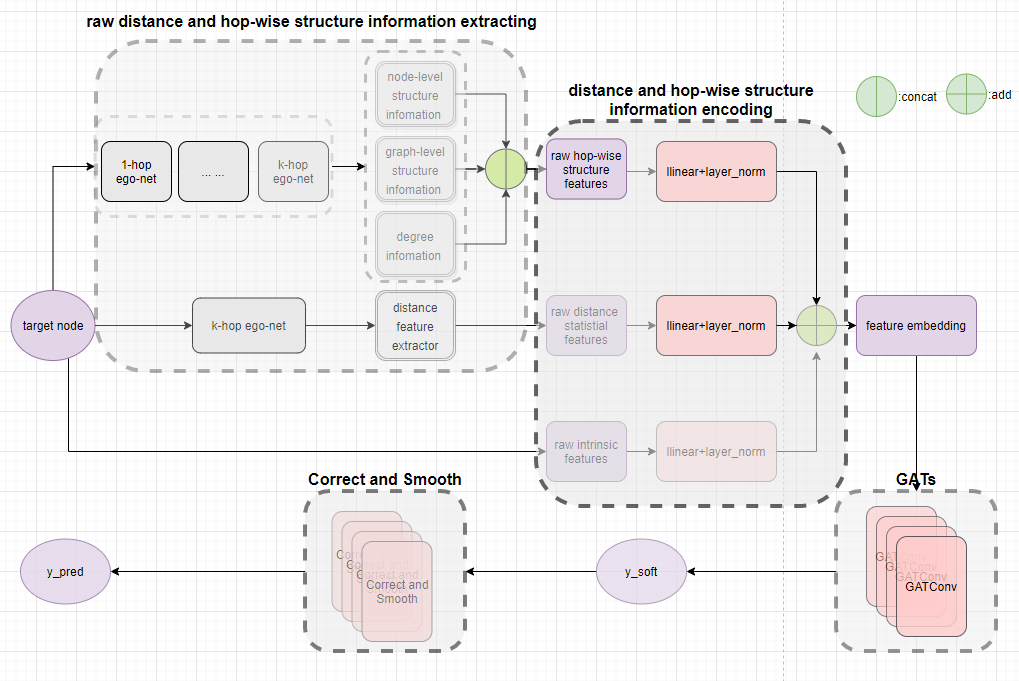
Figure 1: architecture

Figure 1 overall architecture of DHSEGATs

3.2 Preprocessing

3.2.1 Degree Features

Drawing lessons from Graphormer([7]) embeding in-degree and out-degree as centrality feature, we also use in-degree and out-degree but as a part of structure information.

3.2.2 Hop-wise Ego-net’s Node-level and Graph-level Features

As mentioned before, neighbor-averaging GNNs can only catch degree information at best, and degree information is merely one-hop node-level structure information. To catch multi-hop structure information, we first extract $k$ $r$-hop ego-net($r=1,...,k$), then compute their node-level and graph-level structure information. However, many popular structure information has very high computation complexity, for example, the computation complexity of eigenvector centrality is $O(|N|^{3})$, and betweenness centrality’s is $O(|N|*|E|)$(where $|E|$ denotes number of edges). It’s unrealistic to apply to large-scale graph if the preprocessing has very high computation complexity. Therefore, we first investigate computation complexity of popular structure indicators, from which we choose following indicators with $O(|N|)$ computation complexity:

1. Node-level Structure Information: Triangles, Clustering, Square Clustering

Triangles: the number of triangles contains target node in ego-net.

Clustering: $c_{u}=\frac{2T(u)}{deg(u)(deg(u)-1)}$, where $T(u)$ is the number of triangles through node $u$ and $deg(u)$ is the degree of $u$.

Square- clustering:$C_{4}(v)=\frac{\sum_{u=1}^{k_{v}}\sum_{w=u+1}^{k_{v}}q_{v}(u,w)}{\sum_{u=1}^{k_{v}}\sum_{w=u+1}^{k_{v}}[a_{v}(u,w)+q_{v}(u,w)]}$, where $q_v(u,w) $are the number of common neighbors of $u$ and $w$ other than $v$ (ie squares), and $a_{v}(u,w)=(k_{u}-(1+q_{v}(u,w)+\theta_{uv}))+(k_{w}-(1+q_{v}(u,w)+\theta_{uw}))$, where $\theta_{uw}=1$ if $u$ and $w$ are connected and $0$ otherwise.

1. Graph-level Structure Information: Density, Number of Self-loops, Transitivity

Density: $d=\frac{2m}{n(n-1)},$ where $n$ is the number of nodes and $m$ is the number of edges in graph.

Number of self-loops: number of self-loop edges, where a self-loop edge has the same node at both ends.

Transitivity: $T=3\frac{\#triangles}{\#triads}$, where a triad is graph contains of two edges with a shared vertex.

3.2.3 Distance Distributional Features

Distance information is a very important information for attention mechanism. In order to get larger sensitive field of distance information, we first extract $k$-hop ego-net arounds target node, and compute every neighbor node’s unweighted distance in the ego-net to target node to get a distance sequence. However, we cannot directly apply the sequence to GNNs because the sequence is variant and may be very long. As a result, we should encoding it to a fixed length vector beforehand. Technicallly, we can adopt neighbor sampling and padding technique, but this way may corrupt graph’s structure and introduce a virtual node, which may result disastrous consequence in encoding. Hence we adopt an encoding method based on distributional indicators, that is to compute statistics of the sequence. We chose seven statistics, including: maximum, minimum, median, mean, standard deviation, kurtosis, skewness.

3.3 Encoding Distance and Hop-wise Structure Features

In order to encode distance and hop-wise structure information, we first encode distance distributional information ,hop-wise structure feature ,intrinsic feature to same vector space by three linear layers:

$$hd=dist\_encoder(raw\ distance\ distributional\ feature)$$ (1)

$$hs=struc\_encoder(raw\ hop-wise\ structure\ feature)$$ (2)

$$hi=intri\_encoder(raw\ intrinsic\ feature)$$ (3)

In order to avoid one of the there feature dominate the initial encoding vector, layer norm modules are followed:

$$hi=layer\_norm(hi)$$ (4)

$$hd=layer\_norm(hd)$$ (5)

$$hs=layer\_norm(hs)$$ (6)

In order to reduce the spatial complexity, the three encoded vectors are added up and get initial encoding vector as follow:

$$h=hi+hd+hs$$ (7)

3.4 GATs

In this work, we investigate two GAT models: GAT and AGDN. The former is most classical attention model on graph and a generally used baseline model. The latter achieve best performance on ognb-arxiv dataset among single models by combining attention mechanims and graph diffusion process.

3.4.1 GAT

A general form of neighbor-averaging GNN could be written as:

$$h_{i}^{\prime}=UPD_{W}\left(h_{i},AGG_{j\in N(i)}\,MES_{W}\left(h_{i},h_{j},e_{j,i}\right)\right)$$ (8)

where $h$, $AGG$, $MES$ , $UPD$ denote nodes’ representation, aggregating function, message function, and updating function respectively. GAT’s $AGG$ is linear layer, and $MES$ is multi-head attention function. So the attention mechanism in GAT could be described as follow:

$$h_{i}^{\prime}(K)=Pool_{k=1}^{K}h^{\prime}_{ik}$$ (9)

$$h_{i}^{\prime}=\sigma\left(\sum_{j\in\mathcal{N}_{i}}\alpha_{ij}Wh_{j}\right)$$ (10)

$$\alpha_{i,j}=\frac{\exp\left(\sigma\left(\mathbf{a}^{\top}[\mathbf{\Theta}\mathbf{x}_{i}\,\|\,\mathbf{\Theta}\mathbf{x}_{j}]\right)\right)}{\sum_{k\in\mathcal{N}(i)\cup\{i\}}\exp\left(\sigma\left(\mathbf{a}^{\top}[\mathbf{\Theta}\mathbf{x}_{i}\,\|\,\mathbf{\Theta}\mathbf{x}_{k}]\right)\right)}$$ (11)

where $Pool$ denotes pooling function in multi-heads, in the work we use mean pooling function; $K$ denotes number of heads; $\alpha_{ij}$ denotes normalized attention score of source node $j$ on target node $i$ . $\sigma$ denotes activation function.

3.4.2 AGDN

By denoting transition matrix , parameters matrix, attention vector as $\mathbf{T}^{(l)}$, $\mathbf{W}^{(l)},a_{hw}^{(l)}$ respectively, AGDN-HA layer could be defined as ,

$$\mathbf{H}^{(l)}=AGDN(\mathcal{G},\mathbf{H}^{(l-1)},\mathbf{W}^{(l)},a_{hw}^{(l)})$$ (12)

$$\hat{\mathbf{H}}^{(0,l)}=\mathbf{H}^{(l-1)}\mathbf{W}^{(l)}$$ (13)

$$\hat{\mathbf{H}}^{(k,l)}=\mathbf{T}^{(l)}\hat{\mathbf{H}}^{(k-1,l)}$$ (14)

To be more specific, the output of AGDN-HA layer could be written as:

$$\boldsymbol{H}^{(l)}=\sum_{k=0}^{K}\boldsymbol{\Theta}^{(k,l)}\hat{\boldsymbol{H}}^{(k,l)}+\boldsymbol{H}^{(l-1)}\boldsymbol{W}_{r}^{(l)}$$ (15)

$$\Theta^{(k,l)}=diag(\theta^{(k,l)}_{1},...,\theta_{N}^{(k,l)})$$ (16)

$$\theta_{i}^{(k,l)}=\frac{\exp\left(\sigma\left(\left[\hat{H}_{i}^{(0,l)}||\hat{H}_{i}^{(k,l)}\right]\cdot a_{hw}^{(l)}\right)\right)}{\sum_{k=0}^{K}\exp\left(\sigma\left(\left[\hat{H}_{i}^{(0,l)}\|\hat{H}_{i}^{(k,l)}\right]\cdot a_{hw}^{(l)}\right)\right)}$$ (17)

Where $\hat{H}_{i}^{(k,l)}$ denotes representation vector of layer $l$, aggregation $k$, node $i$.

3.5 Correct and Smooth

The reason why we choose Correct and Smooth([29]) among large amouts of label propgation algorithm on GNN is that it has two advantages: 1), Correct and Smooth is such an effective label propagation algorithm that even combing with MLP, it outperforms most of complicate GNN models. 2), Correct and Smooth is a post-processing module that does not disturb base model, and thanks to that we can evaluate base model properly. Correct and Smooth contains of two steps: Correct module corrects the base predictions by modeling correlated error and Smooth module smooths the soft prediction by correlated error.

3.5.1 Correcting

The basic idea of correcting module is that errors in the base prediction to be positively correlated along edges in the graph, In other words, an error at node $i$ increases the chance of a similar error at neighboring nodes of $i$. Denoting error matrix as $E$, we can get:

$$E_{L_{t}}=Z_{L_{t}}-Y_{L_{t}},E_{L_{v}}=0,E_{U}=0$$ (18)

where $L_{t},L_{v},U,Z,Y$ denote training labeled data, validating labeled data, unlabeled data, base predictions, ground-truth labels repectively.

After that, label spreading technique is used to smooth the err:

$$\hat{E}=\underset{W\in\mathbb{R}^{n\times c}}{\arg\min}\operatorname{trace}\left(W^{T}(I-S)W\right)+\mu\|W-E\|_{F}^{2}$$ (19)

Where$S=D^{-1/2}AD^{-1/2}$, $\mathbf{I}$ denote unit matrix.

Add the solution of $(19)$ to $Z$ with some scale method to get corrected prediction:

$$Z^{(r)}=f(Z,\hat{E})$$ (20)

Where $f$ denotes scale and add operation, here we adapt scaled fixed diffusion(FDiff-scale), then we get:

$$Z^{(r)}=Z+s\hat{E}$$ (21)

Where $s$ is a hyperparameter.

3.5.2 Smoothing

Based on the assumption that adjacent nodes in the graph are likely to have similar labels, we can smooth $Z^{(r)}$ to get final predictions. Start with best guess $G$:

$$G_{L_{t}}=Y_{L_{t}},\ \ \ G_{L_{v},U}=Z^{(r)}_{L_{v},U}$$ (22)

And implement following iterating until convergence:

$$G^{(t+1)}=(1-\alpha)G+\alpha SG^{(t)}$$ (23)

Where $G^{(0)}=G$.

The smoothed result then could be used to make final predictions.

4. Experiments

We conduct detailed experiments on ogbn-arxiv dataset to examine the effectiveness of distance and hop-wise structure encoding(DHSE) module, main results are presented below.

4.1 Results

4.1.1 Performance Comparison

Comparing with baseline models, GATs with DHSE and combining with Correct and Smooth get significant improvement. It demonstrates that DHSE provides GATs the high-level multi-hop distance and structure information that GATs cannot catch with original neighbor-averaging mechanism.

Table 1 performance comparison

model	Valid Accuracy	Test Accuracy
AGDN+BoT+self-KD+Correct and Smooth	0.7518 ± 0.0009	0.7431 ± 0.0014
UniMP_v2	0.7506 ± 0.0009	0.7397 ± 0.0015
GAT + Correct and Smooth	0.7484 ± 0.0007	0.7386 ± 0.0014
AGDN (GAT-HA+3_heads)	0.7483 ± 0.0009	0.7375 ± 0.0021
MLP + Correct and Smooth	0.7391 ± 0.0015	0.7312 ± 0.0012
DHSEGAT+Correct and Smooth	0.7441 ± 0.0012	0.7425 ± 0.0016
DHSEAGDN+Correct and Smooth	0.7462 ± 0.0013	0.7439 ± 0.0019

4.1.2 Best Performance of DHSEAGDN and DHSEGAT with and without Correct and Smooth

We argue that DHSE provides GATs the high-level multi-hop distance and structure information that neighbor-averaging mechanism cannot catch, however, initial GAT’s classifier may neglect the information that intrinsic features provide with those information. Therefore, the performance of base model may not significantly improved. But combining with Correct and Smooth, those information could be effectively used and the overall performance be improved.

Since DHSEAGDN and DHSEGAT get their best performance in different hyperparameter setting, so we report the results separately as below. With same hyperparameter setting, the performance of enhanced models (ie, DHSEAGDN and AGDN) and base model (ie, AGDN and GAT) are very close, but with Correct and Smooth, their difference are very significant.

Table 2 best performance of DHSEAGDN with and without Correct and Smooth

model	Valid Accuracy	Test Accuracy
DHSEAGDN	0.7427 ± 0.0007	0.7283 ± 0.0030
DHSEAGDN+Correct and Smooth	0.7462 ± 0.0013	0.7439 ± 0.0019
AGDN	0.7429 ± 0.0010	0.7297 ± 0.0021
AGDN+Correct and Smooth	0.7471 ± 0.0007	0.7387 ± 0.0018

Table 3 best performance of DHSEGAT with and without Correct and Smooth

model	Valid Accuracy	Test Accuracy
DHSEGAT	0.7412 ± 0.0008	0.7261 ± 0.0021
DHSEGAT+Correct and Smooth	0.7441 ± 0.0012	0.7425 ± 0.0016
GAT	0.7419 ± 0.0005	0.7273 ± 0.0012
GAT+Correct and Smooth	0.7440 ± 0.0012	0.7371 ± 0.0023

4.1.3 Marginal Improvement with Same Hyperparameter as AGDN

To demonstrate the marginal improvement of models with DHSE, we test the models with same hyperparameter setting as AGDN([23]), the results are presented as Table 4. We can see that combining with Correct and Smooth, DHSE can improve the performance of base models significantly.

Table 4 marginal improvement of DHSE

model	Valid Accuracy	Test Accuracy
DHSEAGDN	0.7464 ± 0.0008	0.7346 ± 0.0007
DHSEAGDN+Correct and Smooth	0.7485 ± 0.0008	0.7414 ± 0.0010
AGDN	0.7432 ± 0.0007	0.7344 ± 0.0018
AGDN+Correct and Smooth	0.7447 ± 0.0009	0.7398 ± 0.0010
DHSEGAT	0.7448 ± 0.0007	0.7308 ± 0.0014
DHSEGAT+Correct and Smooth	0.7471 ± 0.0006	0.7388 ± 0.0017
GAT	0.7414 ± 0.0005	0.7298 ± 0.0022
GAT+Correct and Smooth	0.7438 ± 0.0006	0.7369 ± 0.0018

4.2 Ablation Study

In this section, we examine the effectiveness of every component of DHSE in improving performance of base model. DHSE contains of three parts: encoding layers, structure information and distance distributional information. The ablation study of the three parts are present as below.

4.2.1 Encoding Layers

From Table 5 we can see that, encoding layers are indivisible part of DHSEGATs. Without encoding layers, their performance are inferior to base model.

Table 5 DHSEGATs without encoding layers

model	Valid Accuracy	Test Accuracy
AGDN+raw features	0.7398 ± 0.0020	0.7303 ± 0.0022
AGDN+raw features+Correct and Smooth	0.7384 ± 0.0023	0.7377 ± 0.0026
GAT+raw features	0.7378 ± 0.0006	0.7244 ± 0.0018
GAT+raw features+Correct and Smooth	0.7407 ± 0.0014	0.7374 ± 0.0020

4.2.2 Structure Information

The strucutre information of DHSE contains of three different level: degree, node-level and graph-level information. From Table 6, Table 7 and Table 8, we can see that degree, node-level structure and graph-level structure information contribute similar marginal improvement to DHSEGATs accordingly.

Table 6 DHSEGATs without degree information

model	Valid Accuracy	Test Accuracy
DHSEAGDN-degree	0.7437 ± 0.0005	0.7315 ± 0.0013
DHSEAGDN-degree+Correct and Smooth	0.7443 ± 0.0010	0.7417 ± 0.0008
DHSEGAT-degree	0.7423 ± 0.0005	0.7286 ± 0.0021
DHSEGAT-degree+Correct and Smooth	0.7447 ± 0.0010	0.7379 ± 0.0022

Table 7 DHSEGATs without node-level structure information

model	Valid Accuracy	Test Accuracy
DHSEAGDN-node	0.7447 ± 0.0008	0.7269 ± 0.0012
DHSEAGDN-node+Correct and Smooth	0.7474 ± 0.0010	0.7425 ± 0.0015
DHSEGAT-node	0.7438 ± 0.0004	0.7301 ± 0.0022
DHSEGAT-node+Correct and Smooth	0.7450 ± 0.0011	0.7402 ± 0.0012

Table 8 DHSEGATs without graph-level structure information

model	Valid Accuracy	Test Accuracy
DHSEAGDN-graph	0.7444 ± 0.0008	0.7290 ± 0.0036
DHSEAGDN-graph+Correct and Smooth	0.7463 ± 0.0016	0.7419 ± 0.0028
DHSEGAT-graph	0.7422 ± 0.0006	0.7265 ± 0.0012
DHSEGAT-graph+Correct and Smooth	0.7450 ± 0.0016	0.7399 ± 0.0019

4.2.3 Distance Distributional Information

From Table 9 we can see that distance distributional information provides indivisible information to DHSEAGDN, but not to DHSEGAT. We can see that without distance distributional information, the performance of DHSEGAT is even improved slightly. We can presume that different model need different information. For GAT, distance information is not indivisible, however for AGDN, distance information is indivisible because of its graph diffusion process.

Table 9 DHSEGATs without distance distributional information

model	Valid Accuracy	Test Accuracy
DHSEAGDN-distance	0.7465 ± 0.0004	0.7315 ± 0.0032
DHSEAGDN-distance+Correct and Smooth	0.7473 ± 0.0014	0.7408 ± 0.0020
DHSEGAT-distance	0.7429 ± 0.0006	0.7303 ± 0.0017
DHSEGAT-distance+Correct and Smooth	0.7443 ± 0.0007	0.7394 ± 0.0020

5. Conclusion

The disadvantage of GNN in catching structure information of graph has been broadly proven, and the ability of structure and distance information to improve performance of GNN has been widely proven as well. Inspired by Graphormer[7], we investigate popular structure indicators‘ computation complexity and propose a structure indicator combination with $O(|N|)$ computation complexity, and propose a distance distributional information encoding scheme. We propose a distance and hop-wise structure information injecting scheme which fits universal GNN models. Detailed experiments shows its ability on improving the expressive power of GNNs.

By detailed experiments, we demonstrate that label information that Correct and Smooth provides is indivisible for DHSE on improving the expressive power of GNNs. Without Correct and Smooth, DHSE can only slightly improve the performance of GATs. However, with Correct and Smooth, DHSE can significantly improve the performance. It implies that DHSE provides GATs the information that neighbor-averaging schema cannot provide, and neighbor-averaging schema cannot effectively use those information but Correct and Smooth can. Moreover, ablation study shows that encoding layers are key compoments of DHSEGATs in improving performance of base model, and every structure information make similar contribution, while distance distributional information is indisvisible part of DHSE.

Reference

re [1] Q. Li, Z. Han, and X.-M. Wu, “Deeper insights into graph convolutional networks for semi-supervised learning,” in Thirty-Second AAAI conference on artificial intelligence, 2018.

pre [2] K. Oono and T. Suzuki, “Graph neural networks exponentially lose expressive power for node classification,” 2019. [Online]. Available: https://arxiv.org/abs/1905.10947

pre [3] N. Dehmamy, A.-L. Barabási, and R. Yu, “Understanding the representation power of graph neural networks in learning graph topology,” 2019. [Online]. Available: https://arxiv.org/abs/1907.05008

pre [4] F. Monti, K. Otness, and M. M. Bronstein, “Motifnet: A motif-based graph convolutional network for directed graphs,” in 2018 IEEE Data Science Workshop (DSW), 2018, pp. 225–228.

pre [5] G. Bouritsas, F. Frasca, S. Zafeiriou, and M. M. Bronstein, “Improving graph neural network expressivity via subgraph isomorphism counting,” 2020. [Online]. Available: https://arxiv.org/abs/2006.09252

pre [6] J. You, J. Gomes-Selman, R. Ying, and J. Leskovec, “Identity-aware graph neural networks,” 2021. [Online]. Available: https://arxiv.org/abs/2101.10320

pre [7] C. Ying et al., “Do Transformers Really Perform Bad for Graph Representation?” 2021. [Online]. Available: https://arxiv.org/abs/2106.05234

pre [8] J. You, R. Ying, and J. Leskovec, “Position-aware graph neural networks,” in International Conference on Machine Learning, 2019, pp. 7134–7143.

pre [9] P. Li, Y. Wang, H. Wang, and J. Leskovec, “Distance encoding: Design provably more powerful neural networks for graph representation learning,” 2020. [Online]. Available: https://arxiv.org/abs/2009.00142

pre [10] E. Alsentzer, S. G. Finlayson, M. M. Li, and M. Zitnik, “Subgraph neural networks,” 2020. [Online]. Available: https://arxiv.org/abs/2006.10538

pre [11] G. Dasoulas, L. D. Santos, K. Scaman, and A. Virmaux, “Coloring graph neural networks for node disambiguation,” 2019. [Online]. Available: https://arxiv.org/abs/1912.06058

pre [12] K. Xu, W. Hu, J. Leskovec, and S. Jegelka, “How powerful are graph neural networks?” 2018. [Online]. Available: https://arxiv.org/abs/1810.00826

pre [13] V. Arvind, F. Fuhlbrück, J. Köbler, and O. Verbitsky, “On weisfeiler-leman invariance: Subgraph counts and related graph properties,” Journal of Computer and System Sciences, vol. 113, pp. 42–59, 2020.

pre [14] Z. Chen, L. Chen, S. Villar, and J. Bruna, “Can graph neural networks count substructures?” 2020. [Online]. Available: https://arxiv.org/abs/2002.04025

pre [15] C. Vignac, A. Loukas, and P. Frossard, “Building powerful and equivariant graph neural networks with structural message-passing,” 2020. [Online]. Available: https://arxiv.org/abs/2006.15107

pre [16] H. Nt and T. Maehara, “Revisiting graph neural networks: All we have is low-pass filters,” 2019. [Online]. Available: https://arxiv.org/abs/1905.09550

pre [17] F. Frasca, E. Rossi, D. Eynard, B. Chamberlain, M. Bronstein, and F. Monti, “Sign: Scalable inception graph neural networks,” 2020. [Online]. Available: https://arxiv.org/abs/2004.11198

pre [18] C. Sun and G. Wu, “Scalable and Adaptive Graph Neural Networks with Self-Label-Enhanced training,” 2021. [Online]. Available: https://arxiv.org/abs/2104.09376

pre [19] P. Veličković, G. Cucurull, A. Casanova, A. Romero, P. Lio, and Y. Bengio, “Graph attention networks,” 2017. [Online]. Available: https://arxiv.org/abs/1710.10903

pre [20] T. Wu, H. Ren, P. Li, and J. Leskovec, “Graph information bottleneck,” 2020. [Online]. Available: https://arxiv.org/abs/2010.12811

pre [21] Z. Hu, Y. Dong, K. Wang, K.-W. Chang, and Y. Sun, “Gpt-gnn: Generative pre-training of graph neural networks,” in Proceedings of the 26th ACM SIGKDD International Conference on Knowledge Discovery & Data Mining, 2020, pp. 1857–1867.

pre [22] Z. Hu, Y. Dong, K. Wang, and Y. Sun, “Heterogeneous graph transformer,” in Proceedings of The Web Conference 2020, 2020, pp. 2704–2710.

pre [23] C. Sun and G. Wu, “Adaptive graph diffusion networks with hop-wise attention,” 2020. [Online]. Available: https://arxiv.org/abs/2012.15024

pre [24] H. Wang and J. Leskovec, “Unifying graph convolutional neural networks and label propagation,” 2020. [Online]. Available: https://arxiv.org/abs/2002.06755

pre [25] M. Qu, Y. Bengio, and J. Tang, “Gmnn: Graph markov neural networks,” in International conference on machine learning, 2019, pp. 5241–5250.

pre [26] H. Gao, J. Pei, and H. Huang, “Conditional random field enhanced graph convolutional neural networks,” in Proceedings of the 25th ACM SIGKDD International Conference on Knowledge Discovery & Data Mining, 2019, pp. 276–284.

pre [27] Q. Zheng et al., “GIPA: General Information Propagation Algorithm for Graph Learning,” 2021. [Online]. Available: https://arxiv.org/abs/2105.06035

pre [28] J. Klicpera, A. Bojchevski, and S. Günnemann, “Predict then propagate: Graph neural networks meet personalized pagerank,” 2018. [Online]. Available: https://arxiv.org/abs/1810.05997

pre [29] Q. Huang, H. He, A. Singh, S.-N. Lim, and A. R. Benson, “Combining label propagation and simple models out-performs graph neural networks,” 2020. [Online]. Available: https://arxiv.org/abs/2010.13993

p