A stableness of resistance model for nonresponse adjustment with callback data

Summary

Nonresponse arises frequently in surveys and follow-ups are routinely made to increase the response rate. In order to monitor the follow-up process, callback data have been used in social sciences and survey studies for decades. In modern surveys, the availability of callback data is increasing because the response rate is decreasing and follow-ups are essential to collect maximum information. Although callback data are helpful to reduce the bias in surveys, such data have not been widely used in statistical analysis until recently. We propose a stableness of resistance assumption for nonresponse adjustment with callback data. We establish the identification and the semiparametric efficiency theory under this assumption, and propose a suite of semiparametric estimation methods including a doubly robust one, which generalize existing parametric approaches for callback data analysis. We apply the approach to a Consumer Expenditure Survey dataset. The results suggest an association between nonresponse and high housing expenditures.

Keywords: Callback; Doubly robust estimation; Missing data; Paradata; Semiparametric efficiency.

1 Introduction

Nonresponse often leads to substantially biased statistical inference and is frequently encountered in surveys and observational studies in many areas of scientific research. It has been a persistent concern of statisticians and applied researchers for many years. The missingness is said to be at random (MAR) or ignorable if it does not depend on the missing values conditional on fully-observed covariates, and otherwise it is called missing not at random (MNAR) or nonignorable. A large body of work for nonresponse adjustment has been based on MAR. However, there is suspicion that the missingness mechanism is MNAR in many situations. For example, social stigma in sensitive questions (e.g., HIV status, income, or drug use) makes nonresponse dependent on unobserved variables. The missing data process and the outcome distribution are identified under MAR, but under MNAR identification in general fails to hold without extra information, which substantially jeopardizes statistical inference. Identification means that the parameter or distribution of interest is uniquely determined from the observed-data distribution; it is crucial for missing data analysis, without which statistical inference may be misleading and is of limited interest. Although one can achieve identification if the impact of the outcome on the missingness is completely known, this should be used rather as a sensitivity analysis because in practice such information is seldom available, see e.g. Robins et al. (2000). Otherwise, identification does not hold even for fully parametric models, except for several fairly restrictive ones (e.g., Heckman, 1979; Miao et al., 2016). For semiparametric and nonparametric models, identification and inference under MNAR essentially require the use of auxiliary data, for example, an instrumental variable (Sun et al., 2018; Liu et al., 2020; Tchetgen Tchetgen and Wirth, 2017) or a shadow variable (D’Haultfœuille, 2010; Wang et al., 2014; Miao and Tchetgen Tchetgen, 2016). Researchers have traditionally sought such auxiliary variables from the sampling frame, but it could be difficult in multipurpose studies where multiple survey variables are concerned and multiple auxiliary variables are necessitated. Moreover, such auxiliary variable methods break down if the auxiliary variables also have missing values due to failure of contact in surveys.

In contrast to the paucity of auxiliary variables in the sampling frame, callback data offer an important source of auxiliary information for nonresponse adjustment. In the presence of nonresponse, the interviewer may continue to contact nonrespondents, and the contact process is recorded with callback data, sometimes called level-of-effort data (Biemer et al., 2013). For instance in the 2018 Consumer Expenditure Survey, the maximum number of contact attempts the interviewers made is about 30, and the number of calls made to contact each unit is recorded with the callback data. Callback data have been widely used in epidemiological, economic, social and political surveys for a long time since the 1940’s. Such data are particularly useful to monitor response rates and to study how design features affect the data collection. Examples include Politz and Simmons (1949); Filion (1976); Drew and Fuller (1980); Lin and Schaeffer (1995); Potthoff et al. (1993); Wood et al. (2006); Jackson et al. (2010); Peress (2010); Biemer et al. (2013); Clarsen et al. (2021), and see Groves and Couper (1998); Olson (2013); Kreuter (2013) for a comprehensive review. Although not all surveys could provide callback data, their availability is increasing in modern surveys. The underlying reason is that the response rate in modern surveys is decreasing and follow-ups are essentially required. Examples include the National Health Interview Survey (NHIS), the National Survey of Family Growth (NSFG), the National Survey on Drug Use and Health (NSDUH), the European Social Survey (ESS), the Behavioral Risk Factor Surveillance System (BRFSS), and the Consumer Expenditure Survey (CES).

However, callback data have not been widely used in statistical analysis until recently, although their usefulness for nonresponse adjustment has been recognized since Politz and Simmons (1949). The callback design is analogous to the two/multi-phase sampling (Deming, 1953) by viewing the follow-ups as the second-phase sample, but it differs in that nonresponse may still occur in the follow-up sample and is possibly not at random. Hence, nonresponse adjustment remains difficult even if callbacks are available, due to the challenge for identification and inference under MNAR. In order to do nonresponse adjustment, the notion of “continuum of resistance” assumes that nonrespondents are more similar to delayed respondents than they are to early respondents, so that the most reluctant respondents are used to approximate the nonrespondents. This assumption has been asserted in social and survey researches for decades despite conflicting evidence of its validity (Lin and Schaeffer, 1995; Clarsen et al., 2021). Other approaches include modeling the joint likelihood of callbacks and frame variables (Biemer et al., 2013); Heckman-type models (Chen et al., 2018; Zhang et al., 2018); sensitivity analysis (Rotnitzky and Robins, 1995 unpublished manuscript; Daniels et al., 2015); etc. Most notably, Alho (1990), Kim and Im (2014), Qin and Follmann (2014), and Guan et al. (2018) use callback data to estimate response propensity scores and propose inverse probability weighted and empirical likelihood-based estimation methods, where they impose a fully parametric linear logistic propensity score model and a common-slope assumption that individual characteristics influence the missingness process in the same way across the survey contacts. These previous approaches rest on strong parametric models to achieve identification, which circumvent the underlying sources for identification and limit their use in complex data application.

In order to further investigate the usefulness of callback data and promote their application, we take a fundamentally nonparametric identification strategy, accompanied with practical parametric/semiparametric estimation methods. Our contributions are threefold. First, we characterize a stableness of resistance assumption and establish the identification under this assumption, which is a nonparametric generalization of the parametric approach of Alho (1990). The stableness of resistance assumption states that the impact of the missing outcome on the response propensity is stable in the first two call attempts. This assumption does not impose parametric functional restrictions on the propensity score, does not restrict the impact of covariates on the missingness, and admits any type (discrete or continuous) of variables. Second, under the stableness of resistance assumption we establish the semiparametric theory, which is for the first time in this field. We characterize the tangent space, the efficient influence function and the semiparametric efficiency bound for estimating a general full-data functional. Third, we propose a suite of semiparametric estimation methods including an inverse probability weighted (IPW) estimator, an outcome regression-based (REG) estimator, and a doubly robust (DR) one. The proposed IPW estimator is a generalization of the calibration estimator of Kim and Im (2014) by allowing for nonlinear propensity score models and call-specific effects of covariates on nonresponse. The IPW and REG estimators rest on correct specification of certain working models; otherwise, they are no longer consistent. However, the doubly robust estimator affords double protection against misspecification of working models: it remains consistent if the working models for either the IPW or the REG estimation is correct, but not necessarily both; moreover, it attains the efficiency bound for the nonparametric model when all working models are correct.

The rest of this paper proceeds as follows. In Section 2, we further discuss the challenge for identification with callback data. In Section 3, we characterize the stableness of resistance assumption for using callback data to identify the full-data distribution and establish the identification results. In Sections 4 and 5, we establish the semiparametric theory and describe the IPW, REG and DR estimators. Section 6 includes extensions to estimation of a general full-data functional and to the setting with multiple callbacks. Sections 7 and 8 include numerical illustrations with simulations and a real data application to the Consumer Expenditure Survey (CES; National Research Council, 2013) dataset, respectively. Section 9 concludes with discussions on other extensions and limitations of the proposed approach.

2 Preliminaries and Challenges to Identification

Throughout the paper, we let $(X,Y)$ denote the frame variables that are released in a survey or observational study for investigation of a particular scientific purpose, where $X$ denotes a vector (possibly a null set) of fully observed covariates and $Y$ the outcome prone to missing values. The frame variables $(X,Y)$ can be either continuous or discrete. Suppose in the data collection process the interviewer has continued to contact a unit until he/she responds or the maximum number of call attempts $K$ is achieved. We let $R_{k}$ denote the availability status of $Y$ after the $k$th call, with $R_{k}=1$ if $Y$ is available after the $k$th call and $R_{k}=0$ otherwise. By this definition, we have $R_{k+1}\geq R_{k}$; because if $R_{k}=1$, i.e. $Y$ is already obtained in the $k$th call, then by definition $R_{k+1}=1\geq R_{k}$. The observations of $(R_{1},\ldots,R_{K})$ recording the response process in the survey are known as callback data. Let ${f}$ denote a generic probability density or mass function. The full data can be viewed as $n$ independent and identically distributed samples from the joint distribution ${f}(X,Y,R_{1},\ldots,R_{K})$, and in the observed data the values of $Y$ with $R_{K}=0$ are missing. Table 1 illustrates the data structure of a survey with callbacks, where the final availability status $R_{K}$ can be created based on the availability status of frame data but the callback data $(R_{1},\ldots,R_{K})$ contain much more information about the response process than solely $R_{K}$ does. To ground ideas, we will focus on the setting with two calls or when only the first two calls are considered for analysis and then discuss the extension to multiple calls in Section 6 and the supplement. Our primary goal is to make inference about the outcome mean $\mu=E(Y)$ based on the observed data and extension to a general functional of the full-data distribution ${f}(X,Y)$ will be considered in Section 6.

Table 1: Data structure of a survey with callbacks; NA denotes missing values

Frame data				Callbacks
ID	$X$	$Y$		$R_{1}$	$R_{2}$	$\ldots$	$R_{K}$
1	$x_{1}$	$y_{1}$		1	1	$\cdots$	1
2	$x_{2}$	$y_{2}$		0	1	$\cdots$	1
$\colon$	$\colon$	NA		0	0	$\cdots$	0
$\colon$	$\colon$	NA		0	0	$\cdots$	0
$n$	$x_{n}$	$y_{n}$		0	0	$\cdots$	1

Traditionally, only the final response status $R_{K}$ is used for missing data analysis. Beyond $R_{K}$, callback data $(R_{1},\ldots,R_{K-1})$ reflect the reluctance of units to respond and how the reluctance is related to the outcome, which is particularly informative about the nonresponse process. However, callback data still do not suffice for identification. Consider a toy example of survey on a binary outcome $Y$ with two calls; then the observed-data distribution is captured by ${f}(Y,R_{1}=1)$ and ${f}(Y,R_{2}=1\mid R_{1}=0)$, which only offers four constraints on five unknown parameters ${f}(Y),{f}(R_{1}=1\mid Y),{f}(R_{2}=1\mid R_{1}=0,Y)$ with $Y=0,1$. Therefore, one cannot identify ${f}(Y,R_{1},R_{2})$ without further restrictions. To achieve identification with callback data, Alho (1990), Kim and Im (2014), and Qin and Follmann (2014) consider a common-slope linear logistic model for the propensity scores.

Example 1 (A common-slope linear logistic model).

Alho (1990) assumes that for $k=1,\ldots,K$,

$$\text{\rm logit }{f}(R_{k}=1\mid R_{k-1}=0,X,Y)=\alpha_{k0}+\alpha_{k1}X+\gamma_{k}Y,\quad\text{with}\quad\alpha_{k1}=\alpha_{1},\quad\gamma_{k}=\gamma.$$ (1)

Hereafter, we let $\text{\rm logit }x=\log\{x/(1-x)\}$ be the logit transformation of $x$ and $\text{\rm expit }x=\exp(x)/\{1+\exp(x)\}$ its inverse. Example 1 is a restrictive model: the propensity score for each callback follows a linear (in parameters) logistic model and the effects of both the covariate $X$ and the outcome $Y$ do not vary across call attempts. Daniels et al. (2015) mention an identification result that allows for call-specific coefficients of $X$ but requires constant coefficients of $Y$ across all call attempts. Guan et al. (2018) relax the common slope assumption by only requiring $\alpha_{11}=\alpha_{21}$ and $\gamma_{1}=\gamma_{2}$. This enables identification with only two call attempts, but their identifying strategy based on a meticulous analysis of the logistic model only admits continuous covariates and outcome. In order to make full use of callback data for nonresponse adjustment, it is of great interest to establish identification for other types of models than the linear logistic model. So far, however, identification and inference of semiparametric and nonparametric propensity score models with callbacks are not available.

3 Identification under a stableness of resistance assumption

3.1 The stableness of resistance assumption

An all-important step for identification under MNAR is to characterize the degree to which the missingness departs from MAR. The odds ratio function is a particularly useful measure widely used in the missing data literature to characterize the association between the outcome and response propensity (e.g. Rotnitzky et al., 2001; Osius, 2004; Chen, 2007; Kim and Yu, 2011; Miao and Tchetgen Tchetgen, 2016; Franks et al., 2020; Malinsky et al., 2020). We define the odds ratio functions for the response propensity in the first and second calls as follows,

$$\Gamma_{1}(X,Y) = \log\frac{{f}(R_{1}=1\mid X,Y){f}(R_{1}=0\mid X,Y=0)}{{f}(R_{1}=0\mid X,Y){f}(R_{1}=1\mid X,Y=0)},$$ (2)

$$\Gamma_{2}(X,Y) = \log\frac{{f}(R_{2}=1\mid R_{1}=0,X,Y){f}(R_{2}=0\mid R_{1}=0,X,Y=0)}{{f}(R_{2}=0\mid R_{1}=0,X,Y){f}(R_{2}=1\mid R_{1}=0,X,Y=0)}.$$ (3)

The odds ratio functions $\Gamma_{1}(X,Y)$ and $\Gamma_{2}(X,Y)$ measure the impact of the outcome on the missingness in the first and second calls, respectively, by quantifying the change in the odds of response caused by a shift of $Y$ from a common reference value $Y=0$ to a specific level while controlling for covariates. Probabilities ${f}(R_{1}=1\mid X,Y=0)$ and ${f}(R_{2}=1\mid R_{1}=0,X,Y=0)$ are referred to as baseline propensity scores evaluated at the reference value $Y=0$. Any other value within the support of $Y$ can be chosen as the reference value. Therefore, the odds ratio function is a measure of the resistance to respond caused by the outcome. A positive odds ratio function evaluated at $(x,y)$ indicates that for participants with $X=x$, those with $Y=y$ are more likely to respond than those with $Y=0$, and a larger odds ratio means a stronger willingness to respond. The setting with odds ratio functions equal to zero corresponds to MAR where the outcome does not influence the response. Our identification strategy rests on the following assumption.

Assumption 1.

• Stableness of resistance: $\Gamma_{1}(X,Y)=\Gamma_{2}(X,Y)=\Gamma(X,Y)$ for some $\Gamma(X,Y)$;

• Positivity: $0<{f}(R_{1}=1\mid X,Y)<1$ and $0<{f}(R_{2}=1\mid R_{1}=0,X,Y)<1$ for all $(X,Y)$.

Condition (ii) is a standard positivity assumption in missing data analysis, which ensures sufficient overlap between nonrespondents and respondents in each call attempt. Condition (i) is the key identifying condition, which reveals that the impact of the outcome on the response propensity remains the same in the first two calls. Whether Condition (i) holds or not does not depend on the choice of the reference value in the definition of the odds ratio functions. Although Assumption 1 is concerned with the missingness process, it in fact imposes certain sophisticated restrictions on the outcome distribution. This is because under MNAR the missingness process is not ancillary to the outcome distribution; see Lemma LABEL:lemma:1 in the supplement for the apparent dependence between the missingness process, the outcome distribution and the odds ratio function.

Similar to various missing data problems, Assumption 1 is untestable based on observed data. Thus, the justification of its validity requires domain-specific knowledge and needs to be investigated on a case-by-case basis. Assumption 1 is motivated from the idea that the individual characteristics may influence the missingness process in the same way across the survey contacts. Similar ideas have been used since Alho (1990), Kim and Im (2014), Qin and Follmann (2014), and Guan et al. (2018). Assumption 1 is plausible if the nonignorable missingness is caused by certain social stigma (or other issues such as difficulty to reach) and the social stigma attached to the units does not change during the first two calls or the contacts are made in a short period of time. Besides, sensitivity analysis can be applied to assess how results would change if Assumption 1 were to be violated; see the simulation and application in Sections 7 and 8, respectively.

The biggest difference between Assumption 1 and Model (1) is that, the former is about social reality that researchers can justify based on domain-specific knowledge, whereas the latter further depends on functional form restrictions that may lack real-world justification. Besides, Assumption 1 has several major differences from Model (1), while includes the latter as a special case. Under Assumption 1 the propensity scores have the following representation:

$${f}(R_{1}=1\mid X,Y) = \text{\rm expit }\{A_{1}(X)+\Gamma(X,Y)\},$$ (4)

$${f}(R_{2}=1\mid R_{1}=0,X,Y) = \text{\rm expit }\{A_{2}(X)+\Gamma(X,Y)\},$$ (5)

where $A_{1}(X)=\text{\rm logit }{f}(R_{1}=1\mid X,Y=0)$ and $A_{2}(X)=\text{\rm logit }{f}(R_{2}=1\mid R_{1}=0,X,Y=0)$ are the logit transformations of the corresponding baseline propensity scores which capture impacts of covariates on the missingness, and $\Gamma(X,Y)$ is the common odds ratio function that measures the impact of the outcome on the missingness in the first and second calls. The functions $A_{1}(X),A_{2}(X),\Gamma(X,Y)$ are unrestricted. Therefore, Assumption 1 admits nonlinear and nonparametric effects of covariates and missing outcomes on the missingness, which is a much larger, and in fact, infinite-dimensional model; it accommodates any types of outcomes. The assessment of Assumption 1 only concerns the first two calls and does not depend on the number of callbacks, while the missingness in the remaining calls are left completely unrestricted; it only requires the effects of missing outcomes, captured by the odds ratio, to be stable, while admiting call-specific impacts of covariates on nonresponse. In contrast, Model (1) is fully parametric and the effects of covariates and missing outcomes on the missingness must be linear, which is a restrictive model indexed by several parameters. Model (1) is a special case of Assumption 1 where $A_{1}(X)=\alpha_{10}+\alpha_{1}^{\mathrm{\scriptscriptstyle T}}X$, $A_{2}(X)=\alpha_{20}+\alpha_{1}^{\mathrm{\scriptscriptstyle T}}X$, and $\Gamma(X,Y)=\gamma Y$ encode the effects of variables on the missingness with the regression coefficients. This is best suited for continuous or binary outcomes, but may not be suitable for other types of outcomes. Model (1) imposes parametric functional restrictions on all contact attempts and assumes stable effects of all variables entering the model; however, this may not hold for the entire time range when $K$ is large or callback data are from a long period. In short, Model (1) is a restrictive model making strong parametric functional restrictions beyond the parameter (e.g. the outcome mean) of interest. Assumption 1 makes much less restrictive assumptions and has much greater flexibility.

3.2 Nonparametric identification

We will show that Assumption 1 suffices for identification of the joint distribution ${f}(X,Y,R_{1},R_{2})$. We first briefly explain why callback data are useful and how to leverage them for identification. Consider identification of $f(Y,R_{1}\mid X)$, which hinges on identification of $f(Y,R_{1}=0\mid X)$, i.e., the missing data distribution in the first call. In the presence of nonignorable missing data, we need to determine the selection bias, captured by

$$\frac{f(Y,R_{1}=1\mid X)}{f(Y,R_{1}=0\mid X)}=\frac{{f}(R_{1}=1\mid X,Y)}{{f}(R_{1}=0\mid X,Y)}.$$

With callback data, a natural idea for estimating this selection bias is to approximate $f(Y,R_{1}=0\mid X)$ with $f(Y,R_{1}=0,R_{2}=1\mid X)$, where $f(Y,R_{1}=0,R_{2}=1\mid X)$ is the distribution of the data obtained in the second call. This is analogous to the two-phase sampling (Deming, 1953). However, the challenge here is that nonresponse still occurs in the second call and is possibly not at random, and as a result, $f(Y,R_{1}=0,R_{2}=1\mid X)$ is not necessarily equal to $f(Y,R_{1}=0\mid X)$ and this crude approximation does not suffice for identification. Nonetheless, under Assumption 1 we are able to characterize and can further identify the bias of this approximation as shown in Proposition 1 and Theorem 1 below.

Proposition 1.

Letting $D(X)=A_{2}(X)-A_{1}(X)$, then under Assumption 1 we have that

$$\frac{{f}(R_{1}=1\mid X,Y)}{{f}(R_{1}=0\mid X,Y)} = \frac{{f}(Y,R_{1}=1\mid X)}{{f}(Y,R_{2}=1,R_{1}=0\mid X)}-\exp\{-D(X)\},$$

$$\frac{{f}(R_{2}=1\mid R_{1}=0,X,Y)}{{f}(R_{2}=0\mid R_{1}=0,X,Y)} = \exp\{D(X)\}\frac{{f}(Y,R_{1}=1\mid X)}{{f}(Y,R_{2}=1,R_{1}=0\mid X)}-1.$$

We prove this result in the supplement. Proposition 1 also implies an inequality:

$$\frac{{f}(Y,R_{1}=1\mid X)}{{f}(Y,R_{2}=1,R_{1}=0\mid X)}>\exp\{-D(X)\},$$ (6)

i.e., given $X$ the density ratio on the left hand side is uniformly bounded from zero. This is a restriction on the observed-data distribution imposed by Assumption 1.

In Proposition 1, ${f}(Y,R_{1}=1\mid X)/{f}(Y,R_{2}=1,R_{1}=0\mid X)$ is used to approximate ${f}(R_{1}=1\mid X,Y)/{f}(R_{1}=0\mid X,Y)$ and the approximation bias is captured by $D(X)$. We can further show that $D(X)$ is identified under Assumption 1, and thus the selection bias ${f}(R_{1}=1\mid X,Y)/{f}(R_{1}=0\mid X,Y)$ is identified, and then the identification of $f(Y,R_{1}\mid X)$ and ${f}(X,Y,R_{1},R_{2})$ is straightforward.

Theorem 1.

Under Assumption 1, $D(X)$ is identified, and as a result, ${f}(X,Y,R_{1},R_{2})$ is identified from the observed-data distribution.

Proof.

Proposition 1 implies that

$$\frac{{f}(R_{2}=0\mid R_{1}=0,X)}{{f}(R_{2}=1\mid R_{1}=0,X)} = \int\frac{{f}(R_{2}=0\mid R_{1}=0,X,Y)}{{f}(R_{2}=1\mid R_{1}=0,X,Y)}{f}(Y\mid R_{2}=1,R_{1}=0,X)dY$$ (7)

$$= \int\left[\frac{\exp\{D(X)\}\cdot{f}(Y,R_{1}=1\mid X)}{{f}(Y,R_{2}=1,R_{1}=0\mid X)}-1\right]^{-1}{f}(Y\mid R_{2}=1,R_{1}=0,X)dY$$

$$\equiv L\{D(X)\}.$$

This is an equation with $D(X)$ unknown while all the other quantities are available from the observed-data distribution. Identification of $D(X)$ can be assessed by checking uniqueness of the solution to this equation. For any fixed $x$ and any $D(x)$ such that (6) is satisfied, $L\{D(x)\}$ is strictly decreasing in $D(x)$ because

$$\frac{\partial L\{D(x)\}}{\partial D(x)}=-\int\frac{\exp\{D(x)\}\frac{{f}(Y,R_{1}=1\mid X=x)}{{f}(Y,R_{2}=1,R_{1}=0\mid X=x)}}{\left[\exp\{D(x)\}\frac{{f}(Y,R_{1}=1\mid X=x)}{{f}(Y,R_{2}=1,R_{1}=0\mid X=x)}-1\right]^{2}}{f}(Y\mid R_{2}=1,R_{1}=0,X=x)dY<0.$$

Therefore, for any fixed $x$ the solution to (7) is unique. Applying this argument to all $x$, then $D(X)$ is identified and ${f}(R_{1}=1\mid X,Y),{f}(R_{2}=1\mid R_{1}=0,X,Y)$ are identified according to Proposition 1. Then it is straightforward to show that ${f}(X,Y)$ and ${f}(X,Y,R_{1},R_{2})$ are identified. ∎

We achieve nonparametric identification of ${f}(X,Y,R_{1},R_{2})$ with callback data under the stableness of resistance assumption. The nonparametric identification elucidates the underlying source for identification with callback data, other than invoking parametric functional restrictions; it extends the application of callback data and opens the way to novel estimation methods. To our knowledge, Assumption 1 is so far the most parsimonious condition characterizing the most flexible model for identification with callbacks, and Theorem 1 is so far the most general identification result. Applying Theorem 1 to the linear logistic model, we immediately obtain the following result.

Proposition 2.

Assuming that $\text{\rm logit }{f}(R_{k}=1\mid R_{k-1}=0,X,Y)=\alpha_{k0}+\alpha_{k1}X+\gamma Y$ for $k=1,2$, then $\alpha_{k0},\alpha_{k1}$, and $\gamma$ are identified.

Proposition 2 generalizes the identification of Model (1) by admitting call-specific coefficients of $X$ in the propensity scores and only requiring the coefficients of $Y$ to be equal for the first two calls. Model (1) also reveals a continuum-of-resistance model where nonrespondents are more similar to late respondents than to early ones due to a common odds ratio for all call attempts. However, in the model in Proposition 2 nonrespondents may depart further from late respondents than from early ones, depending on the form of odds ratio functions in later calls. In this case, continuum-of-resistance models are not suitable.

For estimation, we can in principle first estimate ${f}(Y\mid R_{2}=1,R_{1}=0,X)$, ${f}(Y,R_{2}=1,R_{1}=0\mid X),{f}(Y,R_{1}=1\mid X)$, and ${f}(R_{2}=1\mid R_{1}=0,X)$, then plug them into equation (7) to solve for $D(X)$, and finally obtain the estimate of ${f}(X,Y,R_{1},R_{2})$ according to Proposition 1. The first step can be achieved by standard nonparametric estimation and the third step only involves basic arithmetic; however, solving equation (7) in the second step is in general complicated. In the next section, we consider a parameterization for the joint distribution ${f}(X,Y,R_{1},R_{2})$ and develop feasible estimation methods that only require the working models to be partially correct.

4 Inverse probability weighted and outcome regression-based estimation

4.1 Parameterization

Under Assumption 1, we introduce the following factorization of the joint distribution as the basis for parameterization and estimation.

$${f}(Y,R_{1},R_{2}\mid X) = c_{1}(X)\cdot{f}(R_{1}\mid X,Y=0)\cdot\exp\{(R_{1}-1)\Gamma(X,Y)\}\cdot{f}(Y\mid R_{2}=1,R_{1}=0,X)$$ (8)

$$\cdot\{{f}(R_{2}\mid R_{1}=0,X,Y)\}^{1-R_{1}}\cdot\{{f}(R_{2}=0\mid R_{1}=0,X,Y)\}^{-1},$$

$$c_{1}(X) = \frac{{f}(R_{1}=1\mid X)}{{f}(R_{1}=1\mid X,Y=0)}\frac{1}{E\{1/{f}(R_{2}=0\mid R_{1}=0,X,Y)\mid R_{2}=1,R_{1}=0,X\}},$$

where $c_{1}(X)$ is a normalizing function of $X$ that makes the right hand side of (8) a valid density function. We prove (8) in Lemma LABEL:lemma:1 in the supplement. This factorization enables a convenient and congenial specification of four variationally independent components of the joint distribution:

• two baseline propensity scores ${f}(R_{1}=1\mid X,Y=0)$ and ${f}(R_{2}=1\mid R_{1}=0,X,Y=0)$;

• the odds ratio function $\Gamma(X,Y)$;

• and the outcome distribution for the second call ${f}(Y\mid R_{2}=1,R_{1}=0,X)$.

This kind of factorization of a joint density into a combination of univariate conditionals and odds ratio is widely applicable; see Osius (2004), Chen (2007), Kim and Yu (2011), and Franks et al. (2020) for examples in missing data analysis and causal inference. The joint distribution is determined once given the two baseline propensity scores, the odds ratio, and the second-call outcome distribution.

We consider semiparametric estimation under correct specification of a subset of these four models. For notational convenience, we let $\pi_{1}(X,Y)={f}(R_{1}=1\mid X,Y)$ and $\pi_{2}(X,Y)={f}(R_{2}=1\mid R_{1}=0,X,Y)$ denote the propensity scores, $A_{1}(X)=\text{\rm logit }{f}(R_{1}=1\mid X,Y=0)$ and $A_{2}(X)=\text{\rm logit }{f}(R_{2}=1\mid R_{1}=0,X,Y=0)$ the logit transformations of the corresponding baseline propensity scores, and ${f}_{2}(Y\mid X)={f}(Y\mid R_{2}=1,R_{1}=0,X)$ the outcome model for the second call. Note that $\pi_{1}(X,Y)$ and $\pi_{2}(X,Y)$ are determined by $A_{1}(X),A_{2}(X),\Gamma(X,Y)$ as in equations (4)–(5). We will write $\pi_{1},\pi_{2},A_{1},A_{2},{f}_{2},\Gamma$ for short where it does not cause confusion.

4.2 Inverse probability weighting

We specify parametric working models for two baseline propensity scores $A_{1}(X;\alpha_{1})$, $A_{2}(X;\alpha_{2})$, and the odds ratio function $\Gamma(X,Y;\gamma)$. By definition, we require $\Gamma(X,Y=0;\gamma)=0$. This is equivalent to specifying propensity score models $\pi_{1}(X,Y;\alpha_{1},\gamma)$ and $\pi_{2}(X,Y;\alpha_{2},\gamma)$. The logistic model in Proposition 2 is an example. The following equations characterize the propensity scores,

$$0 = E\left\{\frac{R_{1}}{\pi_{1}}-1\mid X,Y\right\},$$ (9)

$$0 = E\left\{\frac{R_{2}-R_{1}}{\pi_{2}}-(1-R_{1})\mid X,Y\right\},$$ (10)

$$0 = E\left\{\frac{R_{2}-R_{1}}{\pi_{2}}-\frac{1-\pi_{1}}{\pi_{1}}R_{1}\mid X,Y\right\}.$$ (11)

The first equation follows from the definition of $\pi_{1}$ and the other two echo the definition of $\pi_{2}$ by noting that $E\left\{(R_{2}-R_{1})/\pi_{2}-(1-R_{1})\mid X,Y\right\}=E\{(1-R_{1})(R_{2}/\pi_{2}-1)\mid X,Y\}=0$. These three conditional moment equations motivate the following marginal moment equations for estimating $(\alpha_{1},\alpha_{2},\gamma)$:

$$0 = \hat{E}\left[\left\{\frac{R_{1}}{\pi_{1}(\alpha_{1},\gamma)}-1\right\}\cdot V_{1}(X)\right],$$ (12)

$$0 = \hat{E}\left[\left\{\frac{R_{2}-R_{1}}{\pi_{2}(\alpha_{2},\gamma)}-(1-R_{1})\right\}\cdot V_{2}(X)\right],$$ (13)

$$0 = \hat{E}\left[\left\{\frac{R_{2}-R_{1}}{\pi_{2}(\alpha_{2},\gamma)}-\frac{1-\pi_{1}(\alpha_{1},\gamma)}{\pi_{1}(\alpha_{1},\gamma)}R_{1}\right\}\cdot U(X,Y)\right],$$ (14)

where $\hat{E}$ denotes the empirical mean operator and $V_{1}(X)=\partial A_{1}(X;\alpha_{1})/\partial\alpha_{1}$, $V_{2}(X)=\partial A_{2}(X;\alpha_{2})/\partial\alpha_{2}$, $U(X,Y)=\partial\Gamma(X,Y;\gamma)/\partial\gamma$. For instance, in the linear logistic model with $A_{1}(X;\alpha_{1})=(1,X^{\mathrm{\scriptscriptstyle T}})\alpha_{1}$, $A_{2}(X;\alpha_{2})=(1,X^{\mathrm{\scriptscriptstyle T}})\alpha_{2}$, $\Gamma(X,Y;\gamma)=Y\gamma$, one may use $V_{1}(X)=V_{2}(X)=(1,X^{\mathrm{\scriptscriptstyle T}})^{\mathrm{\scriptscriptstyle T}},U(X,Y)=Y$. Note that $V_{1},V_{2},U$ can be chosen as other user-specified functions; see Tsiatis (2006, page 30).

Equations (12)–(14) only involve the observed data. The generalized method of moments (Hansen, 1982) can be implemented to solve these equations. Letting $(\hat{\alpha}_{1,{\rm ipw}},\hat{\alpha}_{2,{\rm ipw}},\hat{\gamma}_{\rm ipw})$ be the nuisance estimators obtained from (12)–(14), $\hat{\pi}_{1}=\pi_{1}(\hat{\alpha}_{1,{\rm ipw}},\hat{\gamma}_{\rm ipw})$ and $\hat{\pi}_{2}=\pi_{2}(\hat{\alpha}_{2,{\rm ipw}},\hat{\gamma}_{\rm ipw})$ the estimated propensity scores, and $\hat{p}_{2}=\hat{\pi}_{1}+\hat{\pi}_{2}(1-\hat{\pi}_{1})$ an estimator of $p_{2}={f}(R_{2}=1\mid X,Y)$, we propose the following IPW estimator of the outcome mean,

$$\hat{\mu}_{\rm ipw}=\hat{E}\left\{\frac{R_{2}}{\hat{p}_{2}}Y\right\}.$$ (15)

Preceding our proposal, Kim and Im (2014) developed a calibration estimator under the common-slope logistic model (1). Our IPW estimator can be viewed as a generalization of the calibration estimator, which can in fact be obtained from our IPW estimator by choosing appropriate functions $V_{1},V_{2},U$. However, the calibration estimator may be biased if the slopes of covariates $X$ differ in the two propensity score models, while our IPW estimator works in this case. We include a numerical simulation comparing these two estimators in Section S4.1 of the supplement. Under the common-slope linear logistic model, Qin and Follmann (2014) and Guan et al. (2018) developed empirical likelihood-based estimation that is convenient to incorporate auxiliary information to achieve higher efficiency; it is of interest to extend their approach to the setting with call-specific slopes for covariates.

4.3 Outcome regression-based estimation

Alternatively, the outcome mean can be obtained by estimation or imputation of the missing values. We specify and fit working models $\pi_{1}(\alpha_{1},\gamma),{f}_{2}(Y\mid X;\beta)$ for the first-call propensity score ${f}(R_{1}=1\mid X,Y)$ and the second-call outcome distribution ${f}(Y\mid X,R_{2}=1,R_{1}=0)$, and impute the missing values with

$${f}(Y\mid X,R_{2}=0) = \frac{\exp(-\Gamma){f}(Y\mid X,R_{2}=1,R_{1}=0)}{E\{\exp(-\Gamma)\mid X,R_{2}=1,R_{1}=0\}},$$ (16)

which is known as the exponential tilting or Tukey’s representation (Kim and Yu, 2011; Vansteelandt et al., 2007; Franks et al., 2020). To obtain the nuisance estimators $(\hat{\beta},\hat{\alpha}_{1,{\rm reg}},\hat{\gamma}_{\rm reg})$, we solve

$$0 = \hat{E}\left\{(R_{2}-R_{1})\cdot\frac{\partial\log f_{2}(Y\mid X;\beta)}{\partial\beta}\right\},$$ (17)

$$0 = \hat{E}\left[\left\{\frac{R_{1}}{\pi_{1}(\alpha_{1},\gamma)}-R_{2}\right\}U(X,Y)-(1-R_{2})E\{U(X,Y)\mid X,R_{2}=0;\beta,\gamma\}\right],$$ (18)

where $E(\cdot\mid X,R_{2}=0;\beta,\gamma)$ is evaluated according to (16) and $U(X,Y)=\{\partial A_{1}(X;\alpha_{1})/\partial\alpha_{1},\partial\Gamma(X,Y;\gamma)/\partial\gamma\}$. Note that $U(X,Y)$ can be chosen as other user-specified functions; see Tsiatis (2006, page 30). Equation (17) is the score equation of ${f}_{2}(Y\mid X;\beta)$. Equation (18) is motivated by the equation $\hat{E}[(1-R_{2})\{U(X,Y)-E\{U(X,Y)\mid R_{2}=0,X\}\}]=0$, but the evaluation of $\hat{E}\{U(X,Y)\}$ is untenable due to missing values of $Y$, and thus we replace with $\hat{E}\{R_{1}U(X,Y)/\pi_{1}\}$. An estimator of the outcome mean by imputing the missing outcome values with $E(Y\mid X,R_{2}=0;\hat{\beta},\hat{\gamma}_{\rm reg})$ is

$$\hat{\mu}_{\rm reg}=\hat{E}\{R_{2}Y+(1-R_{2})E(Y\mid X,R_{2}=0;\hat{\beta},\hat{\gamma}_{\rm reg})\}.$$ (19)

We refer to this approach as the outcome regression-based (REG) estimation, although the first-call propensity score model is also involved.

Guan et al. (2018) have previously proposed an estimator that involves the full-data outcome regression $E(Y\mid X)$ whereas our REG estimation involves $E(Y\mid R_{2}=1,R_{1}=0,X)$ that only concerns the observed data and enjoys the ease for model specification and estimation. Moreover, estimation of their outcome regression model requires estimating the propensity scores for all call attempts, but our REG estimation only requires estimating the first-call propensity score.

Note that (12)–(15) are unbiased estimating equations for $(\alpha_{1},\alpha_{2},\gamma,\mu)$ in model

$${\mathcal{M}}_{\rm ipw}=\{\pi_{1}(\alpha_{1},\gamma)\text{ and }\pi_{2}(\alpha_{2},\gamma)\text{ are correct}\},$$

and (17)–(19) are unbiased estimating equations for $(\beta,\alpha_{1},\gamma,\mu)$ in model

$${\mathcal{M}}_{\rm reg}=\{\pi_{1}(\alpha_{1},\gamma)\text{ and }{f}_{2}(Y\mid X;\beta)\text{ are correct}\}.$$

As a consequence, consistency and asymptotic normality of $(\hat{\alpha}_{1,{\rm ipw}},\hat{\alpha}_{2,{\rm ipw}},\hat{\gamma}_{\rm ipw},\hat{\mu}_{\rm ipw})$ in model ${\mathcal{M}}_{\rm ipw}$ and of $(\hat{\beta},\hat{\alpha}_{1,{\rm reg}},\hat{\gamma}_{\rm reg},\hat{\mu}_{\rm reg})$ in model ${\mathcal{M}}_{\rm reg}$ can be established under standard regularity conditions (see e.g., Newey and McFadden, 1994) by following the theory of estimating equations, which we will not replicate here. Besides, other user-specified functions $\{V_{1}(X),V_{2}(X),U(X,Y)\}$ can be chosen in the estimating equations. See e.g. Tsiatis (2006, page 30) for further details on choices of the user-specified functions. The choice of user-specified functions $V_{1}(X),V_{2}(X),U(X,Y)$ depends on the working models and influences the efficiency of the estimators. In principle, the optimal choice can be obtained by deriving the efficient influence function for the nuisance parameters in models ${\mathcal{M}}_{\rm ipw}$ and ${\mathcal{M}}_{\rm reg}$, respectively. However, the potential prize of attempting to attain local efficiency for nuisance parameters may not always be worth the chase because it depends on correct modeling of additional components of the joint distribution beyond the working models, and as pointed out by Stephens et al. (2014) such additional modeling efforts seldom deliver the anticipated efficiency gain. Besides, consistency of the estimators is undermined if the required working models are incorrect. Therefore, we next propose a doubly robust and locally efficient approach.

5 Semiparametric theory and doubly robust estimation

5.1 Semiparametric theory

We consider the model ${\mathcal{M}}_{\rm npr}$ characterized by Assumption 1,

$${\mathcal{M}}_{\rm npr}=\{{f}(X,Y,R_{1},R_{2}):\text{Assumption \ref{assump:odds} holds; $A_{1}(X),A_{2}(X),\Gamma(X,Y),{f}_{2}(Y\mid X)$ are unrestricted.}\}$$

Although the stableness of resistance assumption does impose an inequality constraint (6) on the observed-data distribution, we refer to ${\mathcal{M}}_{\rm npr}$ as the (locally) nonparametric model because no parametric models are imposed in ${\mathcal{M}}_{\rm npr}$ and as established in the following, the observed-data tangent space under ${\mathcal{M}}_{\rm npr}$ is the entire Hilbert space. We aim to derive the set of influence functions for all regular and asymptotically linear (RAL) estimators of $\mu$ and the efficient influence function under ${\mathcal{M}}_{\rm npr}$. To achieve this goal, the primary step is to derive the observed-data tangent space for model ${\mathcal{M}}_{\rm npr}$. Hereafter, we let $O=(X,Y,R_{1},R_{2})$ if $R_{2}=1$ and $O=(X,R_{1},R_{2})$ if $R_{2}=0$ denote the observed data.

Proposition 3.

The observed-data tangent space for ${\mathcal{M}}_{\rm npr}$ is

$$\mathcal{T}=\{h(O)=R_{1}h_{1}(X,Y)+R_{2}h_{2}(X,Y)+h_{3}(X);E\{h(O)\}=0,E\{h^{2}(O)\}<\infty\},$$

where $h_{1}(X,Y)$, $h_{2}(X,Y)$ and $h_{3}(X)$ are arbitrary measurable and square-integrable functions.

This proposition states that the observed-data tangent space for ${\mathcal{M}}_{\rm npr}$ is the entire Hilbert space of observed-data functions with mean zero and finite variance, equipped with the usual inner product. Hence, the stableness of resistance assumption does not impose any local restriction on the observed-data distribution. As a result, there exits a unique influence function for $\mu$ in model ${\mathcal{M}}_{\rm npr}$, which must be the efficient one. We have derived the closed form for the efficient influence function.

Theorem 2.

The efficient influence function for $\mu$ in the nonparametric model ${\mathcal{M}}_{\rm npr}$ is

$${\rm IF}(O;\mu)=\left\{\frac{R_{2}-R_{1}}{\pi_{2}^{2}}-\frac{1-\pi_{1}}{\pi_{1}}\frac{R_{1}}{\pi_{2}}+\frac{R_{1}}{\pi_{1}}\right\}\left\{Y-\frac{E(Y/\pi_{2}\mid X,R_{2}=0)}{E(1/\pi_{2}\mid X,R_{2}=0)}\right\}+\frac{E(Y/\pi_{2}\mid X,R_{2}=0)}{E(1/\pi_{2}\mid X,R_{2}=0)}-\mu.$$

From Theorem 2, the semiparametric efficiency bound for estimating $\mu$ in ${\mathcal{M}}_{\rm npr}$ is $E\{{\rm IF}(O;\mu)^{2}\}$. A locally efficient estimator attaining this semiparametric efficiency bound can be constructed by plugging nuisance estimators of $\pi_{1},\pi_{2},E(\cdot\mid R_{2}=0,X)$ that converge sufficiently fast into the efficient influence function and then solving $\hat{E}\{{\rm IF}(O;\mu)\}=0$. However, if $X$ has more than two continuous components, one cannot be confident that these nuisance parameters can either be modeled correctly or estimated nonparametrically at rates that are sufficiently fast. It is therefore of interest to develop a doubly robust estimation approach, which delivers valid inferences about the outcome mean provided that a subset but not necessarily all low dimensional models for the nuisance parameters are specified correctly.

5.2 Doubly robust estimation

To construct a doubly robust (DR) estimator, we specify working models $\{A_{1}(X;\alpha_{1}),A_{2}(X;\alpha_{2})$, $\Gamma(X,Y;\gamma)$, ${f}_{2}(Y\mid X;\beta)\}$ and estimate the nuisance parameters by solving

$$0 = \hat{E}\left\{(R_{2}-R_{1})\cdot\frac{\partial\log f_{2}(Y\mid X;\beta)}{\partial\beta}\right\},$$ (20)

$$0 = \hat{E}\left[\left\{\frac{R_{1}}{\pi_{1}(\alpha_{1},\gamma)}-1\right\}\cdot V_{1}(X)\right],$$ (21)

$$0 = \hat{E}\left[\left\{\frac{R_{2}-R_{1}}{\pi_{2}(\alpha_{2},\gamma)}-(1-R_{1})\right\}\cdot V_{2}(X)\right],$$ (22)

$$0 = \hat{E}\left[\left\{\frac{R_{2}-R_{1}}{\pi_{2}(\alpha_{2},\gamma)}-\frac{1-\pi_{1}(\alpha_{1},\gamma)}{\pi_{1}(\alpha_{1},\gamma)}R_{1}\right\}\cdot\left\{U(X,Y)-E(U(X,Y)\mid X,R_{2}=0;\beta,\gamma)\right\}\right],$$ (23)

where $V_{1}(X)=\partial A_{1}(X;\alpha_{1})/\partial\alpha_{1}$, $V_{2}(X)=\partial A_{2}(X;\alpha_{2})/\partial\alpha_{2}$, $U(X,Y)=\partial\Gamma(X,Y;\gamma)/\partial\gamma$. Note that $V_{1},V_{2},U$ can be chosen as other user-specified functions; see discussions in Section 4.3 and Tsiatis (2006, page 30). Let $(\hat{\beta},\hat{\alpha}_{1,{\rm dr}},\hat{\alpha}_{2,{\rm dr}},\hat{\gamma}_{\rm dr})$ denote the solution to (20)–(23) and $\hat{\pi}_{1}=\pi_{1}(\hat{\alpha}_{1,{\rm dr}},\hat{\gamma}_{\rm dr}),\hat{\pi}_{2}=\pi_{2}(\hat{\alpha}_{2,{\rm dr}},\hat{\gamma}_{\rm dr}),$ then an estimator of $\mu$ motivated from the influence function in Theorem 2 is

$$\hat{\mu}_{\rm dr} = \hat{E}\left[\left\{\frac{R_{2}-R_{1}}{\hat{\pi}_{2}^{2}}-\frac{1-\hat{\pi}_{1}}{\hat{\pi}_{1}}\frac{R_{1}}{\hat{\pi}_{2}}+\frac{R_{1}}{\hat{\pi}_{1}}\right\}Y\right]$$ (24)

$$-\hat{E}\left[\left\{\frac{R_{2}-R_{1}}{\hat{\pi}_{2}^{2}}-\frac{1-\hat{\pi}_{1}}{\hat{\pi}_{1}}\frac{R_{1}}{\hat{\pi}_{2}}+\frac{R_{1}}{\hat{\pi}_{1}}-1\right\}\frac{E(Y/\hat{\pi}_{2}\mid X,R_{2}=0;\hat{\beta},\hat{\gamma}_{\rm dr})}{E(1/\hat{\pi}_{2}\mid X,R_{2}=0;\hat{\beta},\hat{\gamma}_{\rm dr})}\right].$$

Equations (20)–(22) for estimating $(\beta,\alpha_{1},\alpha_{2})$ remain the same as (17), (12), and (13) in the IPW and REG estimation, respectively; equation (23) is a doubly robust estimating equation for $\gamma$. We summarize the double robustness of the estimators.

Theorem 3.

Under Assumption 1 and regularity conditions described by Newey and McFadden (1994, Theorems 2.6 and 3.4), $(\hat{\alpha}_{1,{\rm dr}},\hat{\gamma}_{\rm dr},\hat{\mu}_{\rm dr})$ are consistent and asymptotically normal provided one of the following conditions holds:

• $A_{1}(X;\alpha_{1}),\Gamma(X,Y;\gamma)$, and $A_{2}(X;\alpha_{2})$ are correctly specified; or

• $A_{1}(X;\alpha_{1}),\Gamma(X,Y;\gamma)$, and ${f}_{2}(Y\mid X;\beta)$ are correctly specified.

Furthermore, $\hat{\mu}_{\rm dr}$ attains the semiparametric efficiency bound for the nonparametric model ${\mathcal{M}}_{\rm npr}$ at the intersection model ${\mathcal{M}}_{\rm ipw}\cap{\mathcal{M}}_{\rm reg}$ where all models $\{A_{1}(X;\alpha_{1}),A_{2}(X;\alpha_{2}),\Gamma(X,Y;\gamma),{f}_{2}(Y\mid X;\beta)\}$ are correct.

This theorem states that $(\hat{\alpha}_{1,{\rm dr}},\hat{\gamma}_{\rm dr},\hat{\mu}_{\rm dr})$ are doubly robust against misspecification of the second-call baseline propensity score $A_{2}(X;\alpha_{2})$ and the second-call outcome distribution ${f}_{2}(Y\mid X;\beta)$, provided that the first-call propensity score $\pi_{1}(X,Y;\alpha_{1},\gamma)$ (i.e., $A_{1}(X;\alpha_{1})$ and $\Gamma(X,Y;\gamma)$) is correctly specified. Moreover, $\hat{\mu}_{\rm dr}$ is locally efficient if all working models are correct, regardless of the efficiency of the nuisance estimators. The outcome mean estimator $\hat{\mu}_{\rm dr}$ has an analogous form to the conventional augmented inverse probability weighted (AIPW) estimator: the first part is an IPW estimator and the second part is an augmentation term involving the outcome regression model. Compared to the IPW and REG estimators in the previous section, the doubly robust estimator offers one more chance to correct the bias due to model misspecification. However, the DR estimator is not anticipated to have a smaller variance than the IPW or the REG estimator, because ${\mathcal{M}}_{\rm npr}$ is a larger model with a semiparametric efficiency bound no smaller than that of ${\mathcal{M}}_{\rm ipw}$ or ${\mathcal{M}}_{\rm reg}$. Besides, if both $A_{2}(X;\alpha_{2})$ and ${f}_{2}(Y\mid X;\beta)$ are incorrect, the proposed doubly robust estimator will generally also be biased. The odds ratio $\Gamma(X,Y;\gamma)$ is essential for all three proposed estimation methods, because it encodes the degree to which the outcome and the missingness process are correlated. In order to estimate the outcome mean, one must be able to account for this correlation. The first-call baseline propensity score $A_{1}(X;\alpha_{1})$ needs to be correct for estimation of the odds ratio, and as a result, $\hat{\alpha}_{1,{\rm dr}}$ is also doubly robust. If $\pi_{1}(\alpha_{1},\gamma)$ is incorrect, $\hat{\mu}_{\rm dr}$ is in general not consistent even if both $A_{2}(X;\alpha_{2})$ and ${f}_{2}(Y\mid X;\beta)$ are correct—because the latter two models only concern the second call. Variance estimation and confidence intervals for the doubly robust approach also follow from the general theory for estimation equations (see e.g., Newey and McFadden, 1994), which can be constructed based on the normal approximation or bootstrap under standard regularity conditions.

Doubly robust methods have been advocated in recent years for missing data analysis, causal inference, and other problems with data coarsening. Previous proposals have assumed that the odds ratio function $\Gamma(X,Y)$ is either known exactly with the special case of MAR (e.g., Scharfstein et al., 1999; Lipsitz et al., 1999; Tan, 2006; van der Laan and Rubin, 2006; Vansteelandt et al., 2007; Okui et al., 2012), or can be estimated with the aid of an extra instrumental or shadow variable (e.g., Miao and Tchetgen Tchetgen, 2016; Sun et al., 2018; Ogburn et al., 2015). We offer an alternative approach that achieves doubly robust estimation of both the odds ratio model and the outcome mean with the aid of callback data.

If the missingness mechanism is indeed at random, i.e. $\Gamma(X,Y)=0$, then ${f}(X,Y,R_{2})$ is identified without callback data. The efficiency bound for the nonparametric model, with the same observed data of $(X,Y)$ but without the callback data, is the variance of the conventional AIPW influence function:

$${\rm IF}_{\rm aipw}(O;\mu)=\frac{R_{2}}{{f}(R_{2}=1\mid X)}Y-\left\{\frac{R_{2}}{{f}(R_{2}=1\mid X)}-1\right\}E(Y\mid X)-\mu.$$

Under MAR, this efficiency bound does not vary in the presence of callback data.

Proposition 4.

Letting ${\mathcal{M}}^{\rm mar}_{\rm npr}=\{{f}(X,Y,R_{1},R_{2}):{f}(X,Y,R_{1},R_{2})\in{\mathcal{M}}_{\rm npr}\text{ and }\Gamma(X,Y)=0\}$, the efficient influence function for $\mu$ in model $\mathcal{M}^{\rm mar}_{\rm npr}$ is still ${\rm IF}_{\rm aipw}(O;\mu)$.

We prove this result in the supplement. Under MAR callback data do not deliver efficiency gain but bring additional modeling strategies and doubly robust estimators, while under MNAR callback data are useful to improve identification as we have established.

6 Extensions

6.1 Estimation of a general full-data functional

We extend the proposed IPW, REG, and DR methods to estimation of a general smooth full-data functional $\theta$, defined as the unique solution to a given estimating equation $E\{m(X,Y;\theta)\}=0$. Familiar examples include the outcome mean with $m(X,Y;\mu)=Y-\mu$; the least squares coefficient with $m(X,Y;\theta)=X(Y-\theta^{\mathrm{\scriptscriptstyle T}}X)$; and the instrumental variable estimand in causal inference with $m(X,Y;\theta)=Z(Y-\theta^{\mathrm{\scriptscriptstyle T}}W)$, where $W$ and $Z$ are subvectors of $X$, $\theta$ is the causal effect of $W$ on $Y$ and is subject to unmeasured confounding and $Z$ is a set of instrumental variables used for confounding adjustment in causal inference. Given estimators of the nuisance parameters, the IPW and REG estimators of $\theta$ can be obtained by solving

$$0=\hat{E}\left\{\frac{R_{2}}{\hat{p}_{2}}m(X,Y;\theta)\right\},$$

$$0=\hat{E}[R_{2}m(X,Y;\theta)+(1-R_{2})E\{m(X,Y;\theta)\mid X,R_{2}=0;\hat{\beta},\hat{\gamma}_{\rm reg}\}],$$

respectively. Letting $m(\theta)\equiv m(X,Y;\theta)$, the efficient influence function for $\theta$ in model ${\mathcal{M}}_{\rm npr}$ is

$${\rm IF}(O;\theta)=-\left[\frac{\partial E\{m(\theta)\}}{\partial\theta}\right]^{-1}$$

$$\quad\cdot\left[\left\{\frac{R_{2}-R_{1}}{\pi^{2}_{2}}-\frac{1-\pi_{1}}{\pi_{1}}\frac{R_{1}}{\pi_{2}}+\frac{R_{1}}{\pi_{1}}-1\right\}\left\{m(\theta)-\frac{E(m(\theta)/\pi_{2}\mid X,R_{2}=0)}{E(1/\pi_{2}\mid X,R_{2}=0)}\right\}+m(\theta)\right].$$ (25)

We prove this result in the supplement. Then a doubly robust and locally efficient estimator of $\theta$ can be constructed by solving $\hat{E}\{{\rm IF}(O;\theta)\}=0$, after obtaining nuisance estimators from (20)–(23).

6.2 Estimation with multiple callbacks

When multiple calls $(K\geq 3)$ are available, identification of ${f}(X,Y,R_{1},\ldots,R_{K})$ equally holds under Assumption 1, even if the propensity scores and outcome distributions for the third and later call attempts are completely unrestricted. In this case, the proposed IPW, REG, and DR estimation methods developed for the setting with two calls still work but they are agnostic to the observed data after the second call. In the supplement, we extend the proposed IPW, REG, and DR estimators to the setting with multiple callbacks, which can incorporate all observations on $(X,Y)$.

7 Simulation

We evaluate the performance of the proposed estimators and assess their robustness against misspecification of working models and violation of the key identifying assumption via simulations. We conduct simulations for both continuous and binary outcome settings. Simulation results for these two settings are analogous, and to save space, here we only present simulation for the continuous setting and defer the binary setting to Section S4.3 in the supplement.

Let $X=(1,X_{1},X_{2})^{\mathrm{\scriptscriptstyle T}}$ and $\widetilde{X}=(1,X_{1}^{2},X_{2}^{2})$ with $X_{1},X_{2}$ independent following a uniform distribution ${\rm Unif}(-1,1)$. We consider four data generating scenarios according to different choices for the second-call baseline propensity score and the second-call outcome distribution. The following table presents the data generating mechanisms and the working models for estimation.

	Data generating model
	$\pi_{1}=\text{\rm expit }(\alpha_{1}^{\mathrm{\scriptscriptstyle T}}X+\gamma Y),\pi_{2}=\text{\rm expit }(\alpha_{2}^{\mathrm{\scriptscriptstyle T}}W_{1}+\gamma Y),f_{2}(Y\mid X)\thicksim N(\beta^{\mathrm{\scriptscriptstyle T}}W_{2},\sigma^{2})$
	Four scenarios with different choices of $(W_{1},W_{2})$
	TT	FT	TF	FF
	$W_{1}=X,W_{2}=X$	$W_{1}=\widetilde{X},W_{2}=X$	$W_{1}=X,W_{2}=\widetilde{X}$	$W_{1}=\widetilde{X},W_{2}=\widetilde{X}$
$\alpha_{1}^{\mathrm{\scriptscriptstyle T}}$	(-1, 0.5, 0.2)	(-0.3, -0.7, 0.7)	(-1, 1, -0.1)	(-0.3, -0.5, 1)
$\alpha_{2}^{\mathrm{\scriptscriptstyle T}}$	(1, 0.5, 0.2)	(-0.3, 1.9, 0.9)	(0.5, 1, -0.1)	(-0.4, 0.8, 0)
$\beta^{\mathrm{\scriptscriptstyle T}}$	(2.5, 2.3, 1.6)	(-1, 5.4, 4)	(-0.5, 5, -1)	(-1.5, 4, 3)
$\gamma$	0.16	0.1	0.5	0.25
$\sigma$	1.2	2	0.4	0.25
	Working model for estimation
	$\pi_{1}=\text{\rm expit }(\alpha_{1}^{\mathrm{\scriptscriptstyle T}}X+\gamma Y),\pi_{2}=\text{\rm expit }(\alpha_{2}^{\mathrm{\scriptscriptstyle T}}X+\gamma Y),f_{2}(Y\mid X)\thicksim N(\beta^{\mathrm{\scriptscriptstyle T}}X,\sigma^{2})$

Hence, the working model for the second-call baseline propensity score is correct in Scenarios (TT) and (TF), the second-call outcome model is correct in Scenarios (TT) and (FT), and they both are incorrect in Scenario (FF). The first-call baseline propensity score and the odds ratio models are correct in all scenarios. For estimation, we implement the proposed IPW, REG, and DR methods $(\hat{\mu}_{{\rm ipw}}$,$\hat{\mu}_{{\rm reg}},\hat{\mu}_{{\rm dr}})$ to estimate the outcome mean and the odds ratio parameter. We compute the variance of these estimators and then construct the confidence interval based on the normal approximation and evaluate the coverage rate. For comparison, we also implement standard IPW_mar, REG_mar, DR_mar estimators ($\hat{\mu}^{\rm{mar}}_{{\rm ipw}}$,$\hat{\mu}^{\rm{mar}}_{{\rm reg}},\hat{\mu}^{\rm{mar}}_{{\rm dr}}$) that are based on MAR, with the number of callbacks included as an additional covariate.

For each scenario, we replicate 1000 simulations at sample size 3000. Figures 1 and 2 show the bias for estimators of the outcome mean and the odds ratio parameter, respectively, and Table 2 shows the coverage rates for the corresponding confidence intervals. In Scenario (TT) where all working models are correct, all three proposed estimators have little bias and the 95% confidence intervals have coverage rates close to 0.95; in Scenario (FT) the second-call baseline propensity score model is incorrect but the second-call outcome model is correct, then the IPW estimator has large bias with coverage rate well below 0.95 and the REG estimator has little bias with the coverage rate close to 0.95; conversely, in Scenario (TF) the second-call baseline propensity score model is correct but the second-call outcome model is incorrect, then the IPW estimator has little bias with an appropriate coverage rate and the REG estimator has large bias with an undersized coverage rate. The DR estimator has little bias with appropriate coverage rates in all the three scenarios when at least one of these two working models is correct. In Scenario (FF) where both working models are incorrect, all three proposed estimators are biased. These numerical results show the robustness of $\hat{\mu}_{{\rm dr}}$ against partial misspecification of working models. We compare the standard deviations of the three proposed estimators in Table LABEL:tbl:sd in Section S4.2 of supplement, which are close when all working models are correct. However, the three standard MAR estimators have large bias in all four scenarios even if the number of callbacks is included as a covariate. Therefore, we recommend the proposed three methods for nonresponse adjustment with callback data, and we suggest to use different working models to gain more robust inferences.

In addition to model misspecification, we also evaluate sensitivity of the inference against violation of the identifying assumption. In Section S4.2 of the supplement, we include a sensitivity analysis to evaluate the performance of the proposed estimators when call-specific odds ratios arise, i.e., the stableness of resistance assumption is not met. The difference between the odds ratios is used as the sensitivity parameter to capture the degree to which the stableness of resistance assumption is violated. The proposed estimators exhibit small bias when the difference of odds ratios varies within a moderate range but it could become severe if there were a big gap between the odds ratios. To obtain reliable inferences in practice, we recommend such sensitivity analysis for assessing robustness of inference against violation of the stableness of resistance assumption.

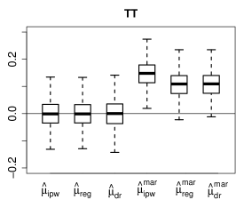
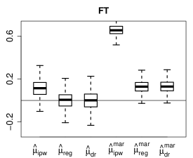
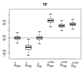
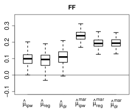
Figure 1: Bias for estimators of $\mu$ in the continuous outcome setting.

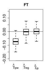
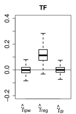
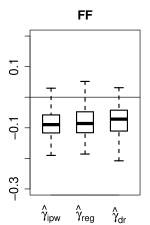
Figure 2: Bias for estimators of $\gamma$ in the continuous outcome setting.

Table 2: Coverage rate of $95\%$ confidence interval in the continuous outcome setting

	$\mu$							$\gamma$
Scenarios	IPW	REG	DR	IPWmar	REGmar	DRmar		IPW	REG	DR
TT	0.955	0.955	0.950	0.109	0.362	0.363		0.955	0.955	0.956
FT	0.622	0.947	0.947	0.000	0.034	0.075		0.308	0.964	0.945
TF	0.944	0.125	0.952	0.000	0.000	0.000		0.947	0.501	0.944
FF	0.285	0.445	0.300	0.000	0.000	0.000		0.495	0.620	0.685

8 Real data application

The Consumer Expenditure Survey (CES; National Research Council, 2013) is a nationwide survey conducted by the U.S. Bureau of Labor Statistics to find out how American households make and spend money. It comprises two surveys: the Quarterly Interview Survey on large and recurring expenditures such as rent and utilities, and the Diary Survey on small and high frequency purchases, such as food and clothing. The survey data are released annually since 1980, which contain detailed callback history. We analyze the public-use microdata from the Quarterly Interview Survey in the fourth quarter of 2018, available from https://www.bls.gov/cex/pumd_data.htm#csv. The nonresponse of frame variables is concurrent due to contact failure or refusal and no fully-observed baseline covariates are available in this dataset. For illustration, we analyze this dataset to study the expenditures on housing and on utilities, fuels and public services. This survey contains 9986 households and 277 of them with extremely large or small expenditures are removed in our analysis. The maximum number of contact attempts the interviewers made in this survey is about 30. Figure 3 (a) shows the cumulative response rate. The overall response rate is about 0.6 and 80% of the respondents completed the survey within the first five contact attempts. Let $(Y_{1},Y_{2})$ denote the logarithm of the expenditure on housing and on utilities, fuels and public services, respectively. Figure 3 (b) shows the mean of $(Y_{1},Y_{2})$ for respondents to each call attempt. The mean of $Y_{1}$ for respondents gradually increases with the number of contacts, and the mean of $Y_{2}$ has a sharp increase in the second and third contacts and fluctuates in later contacts. These results suggest that the delayed respondents are likely to have higher expenditures and the nonresponse is likely dependent on the expenditures, in particular, on $Y_{1}$.

(a) Cumulative response rate

(b) Outcomes mean

Figure 3: Response rates and outcomes mean for respondents in the CES application.

We apply the proposed methods to estimate the outcomes mean $\mu=(\mu_{1},\mu_{2})=(E(Y_{1}),E(Y_{2}))$. Analogous to previous survey studies (e.g., Qin and Follmann, 2014; Boniface et al., 2017), we split the contact attempts into two stages: 1–2 calls (early contact) and 3+ calls (late contact). Among the 9709 households we analyze, 1992 responded in the first stage, 3287 responded later, and 4430 never responded. We fit the data with working models $\pi_{1}=\text{\rm expit }(\alpha_{1}+\gamma_{1}Y_{1}+\gamma_{2}Y_{2}),\pi_{2}=\text{\rm expit }(\alpha_{2}+\gamma_{1}Y_{1}+\gamma_{2}Y_{2})$ and ${f}_{2}(Y)\thicksim N(\mu,\Sigma)$, and apply the proposed IPW, REG, and DR methods to estimate the outcomes mean. The common odds ratio parameters $(\gamma_{1},\gamma_{2})$ reveal that the resistance to respond caused by the outcomes remain the same in these two contact stages. We also compute the complete-case (CC) sample mean and apply standard inverse probability weighting, regression and doubly robust estimation methods that are based on MAR and include the number of contacts as a covariate, which are respectively denoted by IPW_mar, REG_mar, and DR_mar.

Table 3 presents the estimates. The DR point estimate of $\mu_{1}$ is 7.842 with 95% confidence interval (7.800, 7.884), and of $\mu_{2}$ is 6.345 with (6.296, 6.393). The CC estimate of $\mu_{1}$ is 7.756 (7.734, 7.778) and of $\mu_{2}$ is 6.285 (6.264, 6.306); the DR_mar estimate of $\mu_{1}$ is 7.767 (7.744, 7.790) and of $\mu_{2}$ is 6.287 (6.266, 6.309). The IPW and REG methods produce estimates close to DR; however, the CC and standard MAR estimates of the outcomes mean, in particular of $\mu_{1}$, are well below the DR estimate. As shown in Figure 3 (b), this can be partially explained by the fact that the outcomes mean in early respondents is lower than in the delayed, and therefore, the outcomes mean in the respondents is likely lower than in the nonrespondents. The estimation results of the odds ratio parameters reinforce this conjecture: the IPW, REG, and DR estimates of the odds ratio parameters are all negative, suggesting that high-spending people are more reluctant to respond or more difficult to contact. The odds ratio estimate for expenditure on housing is statistically significant at level 0.01, although it is not significant for expenditure on utilities, fuels and public services. This is evidence for missingness not at random. These results indicate that the expenditure on housing play a more important role in the response process; this may be because the survey takes personal home visit as one of the main modes of interview and people with high expenditure on housing are more difficult to reach. Increasing the variety of interview modes may potentially alleviate such nonignorable nonresponse.

Table 3: Point estimate, 95% confidence interval, and p-value for the CES application

	$\mu_{1}$								$\gamma_{1}$
	IPW	REG	DR	IPWmar	REGmar	DRmar	CC		IPW	REG	DR
Estimate	7.859	7.861	7.842	7.767	7.769	7.767	7.756		-0.269	-0.258	-0.238
CI or p-value	(7.785, 7.932)	(7.810, 7.912)	(7.800, 7.884)	(7.744, 7.789)	(7.746, 7.791)	(7.744, 7.790)	(7.734, 7.778)		0.004	0.001	0
	$\mu_{2}$								$\gamma_{2}$
	IPW	REG	DR	IPWmar	REGmar	DRmar	CC		IPW	REG	DR
Estimate	6.346	6.350	6.345	6.287	6.288	6.287	6.285		-0.028	-0.042	-0.056
CI or p-value	(6.269, 6.423)	(6.297, 6.403)	(6.296, 6.393)	(6.266 , 6.309)	(6.267, 6.310)	(6.266, 6.309)	(6.264, 6.306)		0.812	0.658	0.521

We further conduct sensitivity analysis to assess robustness of the above results against violation of the stableness of resistance assumption. The sensitivity analysis shows that our results are not sensitive to mild violations of the stableness of resistance assumption. In particular, when the sensitivity parameter varies within a moderate range, the DR estimate of $\mu_{1}$ remains larger than the complete-case (CC) sample mean and the estimates based on MAR, and the estimate of $\gamma_{1}$ remains significantly negative. Such results reinforce our finding that high-spending people are more reluctant to respond or more difficult to contact. Details of the sensitivity analysis are relegated to Section S5 of the supplement.

9 Discussion

We establish a novel framework for nonresponse adjustment with callback data, which further illustrates the usefulness and extends the application of callback data. Although not all surveys provide callback data, their availability is increasing in modern surveys. The stableness of resistance assumption is key to our framework. Under this assumption, we establish nonparametric identification and propose a suite of novel estimators including a doubly robust one, which extend previous parametric approaches and further elucidate the underlying source for nonresponse adjustment with callback data. We caution that the stableness of resistance assumption is untestable based on observed data. Therefore, analogous to various missing data problems (Molenberghs et al., 2008; Miao and Tchetgen Tchetgen, 2016; Sun et al., 2018), its validity should be justified based on domain-specific knowledge and needs to be investigated on a case-by-case basis. We have clarified the motivation, implication and limitation of the stableness of resistance assumption to facilitate the justification in practice. Even if the assumption does not hold, our approach constitutes a valid test of whether the missingness is entirely MAR–because the stableness of resistance assumption naturally holds under the null hypothesis of MAR. Besides, sensitivity analysis is warranted to assess robustness of inference against violation of the assumption.

We have employed an odds ratio parameterization and adopted practical parametric working models in the IPW, REG and DR estimators. There exist other parameterizations and we describe estimation under an alternative parameterization in Section S1 in the supplement. Kang and Schafer (2007) cautioned for potentially disastrous bias of certain DR estimators under MAR when all working models are incorrect. However, previous authors have proposed alternative constructions of nuisance estimators and DR estimators to alleviate this problem, see e.g. Tan (2010); Vermeulen and Vansteelandt (2015); Tsiatis et al. (2011) and the discussions alongside Kang and Schafer (2007). Besides, multiply robust estimation in the sense of Vansteelandt et al. (2007) is also of interest. In addition, our nonparametric identification result opens the way to more sophisticated estimation methods built on complex nonparametric models, such as series or sieve estimation. The doubly robust influence function enjoys an advantage that it admits nuisance estimators with convergence rates considerably slower than $n^{1/2}$ while delivering valid $n^{1/2}$ inference for the functional of interest. For instance, flexible, data-adaptive machine learning or nonparametric methods for estimation of nuisance parameters can be used provided that the nuisance estimators have mean squared error of order smaller than $n^{-1/4}$. Such results have been well-documented (e.g., Benkeser et al., 2017; Kennedy et al., 2017; Athey et al., 2018; Tan, 2020; Rotnitzky et al., 2021; Dukes and Vansteelandt, 2021). For large to high-dimensional covariates, a heuristic approach for variable selection is to include penalties (e.g. LASSO) into the optimization of estimating equations for the nuisance parameters (e.g. Garcia et al., 2010; Fang and Shao, 2016). However, there remain challenges to the variable selection in the presence of nonignorable missing data and callbacks. It is of interest to incorporate these approaches to improve the proposed estimation methods.

We considered a single action response process—a call attempt either succeeds or fails; however, there may exist several dispositions, e.g., interview, refusal, other non-response or final non-contact (Biemer et al., 2013). Concurrent nonresponse is often the case when the missingness is due to failure of contact, but in practice different frame variables may be observed in different call attempts. In this case one may combine the callback design and the graphical model (e.g., Sadinle and Reiter, 2017; Malinsky et al., 2020; Mohan and Pearl, 2021) to account for complex patterns of missingness. In addition to nonresponse adjustment, callback data are also useful for the design and organization of surveys, e.g., allocation of time and staff resources. The integration of the callback design and other tools (e.g., instrumental variables) may be useful for handling simultaneous problems of nonresponse and confounding or other deficiencies in survey and observational studies. It is of interest to pursue these extensions.

Supplementary material

Supplementary material online includes estimation under an alternative parameterization, estimation with multiple callbacks, proof of theorems, propositions, and important equations, additional simulation and real data analysis results, and codes and data for reproducing the simulations and applications.

References

- Alho (1990) Alho, J. M. (1990). Adjusting for nonresponse bias using logistic regression. Biometrika 77, 617–624.
- Athey et al. (2018) Athey, S., G. W. Imbens, and S. Wager (2018). Approximate residual balancing: debiased inference of average treatment effects in high dimensions. Journal of the Royal Statistical Society: Series B 80, 597–623.
- Benkeser et al. (2017) Benkeser, D., M. Carone, M. V. D. Laan, and P. Gilbert (2017). Doubly robust nonparametric inference on the average treatment effect. Biometrika 104, 863–880.
- Biemer et al. (2013) Biemer, P. P., P. Chen, and K. Wang (2013). Using level-of-effort paradata in non-response adjustments with application to field surveys. Journal of the Royal Statistical Society: Series A 176, 147–168.
- Boniface et al. (2017) Boniface, S., S. Scholes, N. Shelton, and J. Connor (2017). Assessment of non-response bias in estimates of alcohol consumption: Applying the continuum of resistance model in a general population survey in england. PloS ONE 12, e0170892.
- Chen et al. (2018) Chen, B., P. Li, and J. Qin (2018). Generalization of Heckman selection model to nonignorable nonresponse using call-back information. Statistica Sinica 28, 1761–1785.
- Chen (2007) Chen, H. Y. (2007). A semiparametric odds ratio model for measuring association. Biometrics 63, 413–421.
- Clarsen et al. (2021) Clarsen, B., J. C. Skogen, T. S. Nilsen, and L. E. Aarø (2021). Revisiting the continuum of resistance model in the digital age: a comparison of early and delayed respondents to the norwegian counties public health survey. BMC Public Health 21, 730.
- Daniels et al. (2015) Daniels, M. J., D. Jackson, W. Feng, and I. R. White (2015). Pattern mixture models for the analysis of repeated attempt designs. Biometrics 71, 1160–1167.
- Deming (1953) Deming, W. E. (1953). On a probability mechanism to attain an economic balance between the resultant error of response and the bias of nonresponse. Journal of the American Statistical Association 48(264), 743–772.
- D’Haultfœuille (2010) D’Haultfœuille, X. (2010). A new instrumental method for dealing with endogenous selection. Journal of Econometrics 154, 1–15.
- Drew and Fuller (1980) Drew, J. and W. A. Fuller (1980). Modeling nonresponse in surveys with callbacks. In Proceedings of the Section on Survey Research Methods of the American Statistical Association, pp. 639–642.
- Dukes and Vansteelandt (2021) Dukes, O. and S. Vansteelandt (2021). Inference for treatment effect parameters in potentially misspecified high-dimensional models. Biometrika 108, 321–334.
- Fang and Shao (2016) Fang, F. and J. Shao (2016). Model selection with nonignorable nonresponse. Biometrika 103, 861–874.
- Filion (1976) Filion, F. (1976). Exploring and correcting for nonresponse bias using follow-ups of non respondents. Pacific Sociological Review 19, 401–408.
- Franks et al. (2020) Franks, A. M., A. D’Amour, and A. Feller (2020). Flexible sensitivity analysis for observational studies without observable implications. Journal of the American Statistical Association 115, 1730–1746.
- Garcia et al. (2010) Garcia, R. I., J. G. Ibrahim, and H. Zhu (2010). Variable selection for regression models with missing data. Statistica Sinica 20(1), 149.
- Groves and Couper (1998) Groves, R. M. and M. P. Couper (1998). Nonresponse in Household Interview Surveys. John Wiley & Sons.
- Guan et al. (2018) Guan, Z., D. H. Leung, and J. Qin (2018). Semiparametric maximum likelihood inference for nonignorable nonresponse with callbacks. Scandinavian Journal of Statistics 45, 962–984.
- Hansen (1982) Hansen, L. P. (1982). Large sample properties of generalized method of moments estimators. Econometrica 50, 1029–1054.
- Heckman (1979) Heckman, J. J. (1979). Sample selection bias as a specification error. Econometrica 47, 153–161.
- Jackson et al. (2010) Jackson, D., I. R. White, and M. Leese (2010). How much can we learn about missing data?: an exploration of a clinical trial in psychiatry. Journal of the Royal Statistical Society: Series A 173, 593–612.
- Kang and Schafer (2007) Kang, J. D. and J. L. Schafer (2007). Demystifying double robustness: A comparison of alternative strategies for estimating a population mean from incomplete data. Statistical Science 22, 523–539.
- Kennedy et al. (2017) Kennedy, E. H., Z. Ma, M. D. McHugh, and D. S. Small (2017). Non-parametric methods for doubly robust estimation of continuous treatment effects. Journal of the Royal Statistical Society: Series B 79, 1229–1245.
- Kim and Im (2014) Kim, J. K. and J. Im (2014). Propensity score adjustment with several follow-ups. Biometrika 101, 439–448.
- Kim and Yu (2011) Kim, J. K. and C. L. Yu (2011). A semiparametric estimation of mean functionals with nonignorable missing data. Journal of the American Statistical Association 106, 157–165.
- Kreuter (2013) Kreuter, F. (2013). Improving surveys with paradata. New Jersey, Hoboken: John Wiley & Sons.
- Lin and Schaeffer (1995) Lin, I.-F. and N. C. Schaeffer (1995). Using survey participants to estimate the impact of nonparticipation. Public Opinion Quarterly 59, 236–258.
- Lipsitz et al. (1999) Lipsitz, S. R., J. G. Ibrahim, and L. P. Zhao (1999). A weighted estimating equation for missing covariate data with properties similar to maximum likelihood. Journal of the American Statistical Association 94, 1147–1160.
- Liu et al. (2020) Liu, L., W. Miao, B. Sun, J. Robins, and E. Tchetgen Tchetgen (2020). Identification and inference for marginal average treatment effect on the treated with an instrumental variable. Statistica Sinica 30, 1517–1541.
- Malinsky et al. (2020) Malinsky, D., I. Shpitser, and E. J. Tchetgen Tchetgen (2020). Semiparametric inference for non-monotone missing-not-at-random data: the no self-censoring model. Journal of the American Statistical Association.
- Miao et al. (2016) Miao, W., P. Ding, and Z. Geng (2016). Identifiability of normal and normal mixture models with nonignorable missing data. Journal of the American Statistical Association 111, 1673–1683.
- Miao and Tchetgen Tchetgen (2016) Miao, W. and E. Tchetgen Tchetgen (2016). On varieties of doubly robust estimators under missingness not at random with a shadow variable. Biometrika 103, 475–482.
- Mohan and Pearl (2021) Mohan, K. and J. Pearl (2021). Graphical models for processing missing data. Journal of the American Statistical Association 116, 1023–1037.
- Molenberghs et al. (2008) Molenberghs, G., C. Beunckens, C. Sotto, and M. G. Kenward (2008). Every missingness not at random model has a missingness at random counterpart with equal fit. Journal of the Royal Statistical Society: Series B 70, 371–388.
- National Research Council (2013) National Research Council (2013). Measuring what we spend: Toward a new consumer expenditure survey. National Academies Press.
- Newey and McFadden (1994) Newey, W. K. and D. McFadden (1994). Large sample estimation and hypothesis testing. In R. F. Engle and D. L. McFadden (Eds.), Handbook of Econometrics, Volume 4, pp. 2111–2245. Amsterdam: Elsevier.
- Ogburn et al. (2015) Ogburn, E. L., A. Rotnitzky, and J. M. Robins (2015). Doubly robust estimation of the local average treatment effect curve. Journal of the Royal Statistical Society. Series B 77, 373–396.
- Okui et al. (2012) Okui, R., D. S. Small, Z. Tan, and J. M. Robins (2012). Doubly robust instrumental variable regression. Statistica Sinica 22, 173–205.
- Olson (2013) Olson, K. (2013). Paradata for nonresponse adjustment. The Annals of the American Academy of Political and Social Science 645, 142–170.
- Osius (2004) Osius, G. (2004). The association between two random elements: A complete characterization and odds ratio models. Metrika 60, 261–277.
- Peress (2010) Peress, M. (2010). Correcting for survey nonresponse using variable response propensity. Journal of the American Statistical Association 105, 1418–1430.
- Politz and Simmons (1949) Politz, A. and W. Simmons (1949). An attempt to get the “not at homes” into the sample without callbacks. Journal of the American Statistical Association 44, 9–16.
- Potthoff et al. (1993) Potthoff, R. F., K. G. Manton, and M. A. Woodbury (1993). Correcting for nonavailability bias in surveys by weighting based on number of callbacks. Journal of the American Statistical Association 88, 1197–1207.
- Qin and Follmann (2014) Qin, J. and D. A. Follmann (2014). Semiparametric maximum likelihood inference by using failed contact attempts to adjust for nonignorable nonresponse. Biometrika 101, 985–991.
- Robins et al. (2000) Robins, J. M., A. Rotnitzky, and D. O. Scharfstein (2000). Sensitivity analysis for selection bias and unmeasured confounding in missing data and causal inference models. In Statistical Models in Epidemiology, the Environment, and Clinical Trials, pp. 1–94. Springer.
- Rotnitzky et al. (2001) Rotnitzky, A., D. Scharfstein, T.-L. Su, and J. Robins (2001). Methods for conducting sensitivity analysis of trials with potentially nonignorable competing causes of censoring. Biometrics 57, 103–113.
- Rotnitzky et al. (2021) Rotnitzky, A., E. Smucler, and J. M. Robins (2021). Characterization of parameters with a mixed bias property. Biometrika 108, 231–238.
- Sadinle and Reiter (2017) Sadinle, M. and J. P. Reiter (2017). Itemwise conditionally independent nonresponse modelling for incomplete multivariate data. Biometrika 104, 207–220.
- Scharfstein et al. (1999) Scharfstein, D. O., A. Rotnitzky, and J. M. Robins (1999). Adjusting for nonignorable drop-out using semiparametric nonresponse models. Journal of the American Statistical Association 94, 1096–1120.
- Stephens et al. (2014) Stephens, A., E. Tchetgen Tchetgen, and V. De Gruttola (2014). Locally efficient estimation of marginal treatment effects when outcomes are correlated: is the prize worth the chase? The International Journal of Biostatistics 10, 59–75.
- Sun et al. (2018) Sun, B., L. Liu, W. Miao, K. Wirth, J. Robins, and E. Tchetgen Tchetgen (2018). Semiparametric estimation with data missing not at random using an instrumental variable. Statistica Sinica 28, 1965–1983.
- Tan (2006) Tan, Z. (2006). A distributional approach for causal inference using propensity scores. Journal of the American Statistical Association 101, 1619–1637.
- Tan (2010) Tan, Z. (2010). Bounded, efficient and doubly robust estimation with inverse weighting. Biometrika 97, 661–682.
- Tan (2020) Tan, Z. (2020). Model-assisted inference for treatment effects using regularized calibrated estimation with high-dimensional data. The Annals of Statistics 48, 811–837.
- Tchetgen Tchetgen and Wirth (2017) Tchetgen Tchetgen, E. J. and K. E. Wirth (2017). A general instrumental variable framework for regression analysis with outcome missing not at random. Biometrics 73, 1123–1131.
- Tsiatis (2006) Tsiatis, A. (2006). Semiparametric Theory and Missing Data. New York: Springer.
- Tsiatis et al. (2011) Tsiatis, A. A., M. Davidian, and W. Cao (2011). Improved doubly robust estimation when data are monotonely coarsened, with application to longitudinal studies with dropout. Biometrics 67, 536–545.
- van der Laan and Rubin (2006) van der Laan, M. J. and D. Rubin (2006). Targeted maximum likelihood learning. The International Journal of Biostatistics 2(1).
- Vansteelandt et al. (2007) Vansteelandt, S., A. Rotnitzky, and J. Robins (2007). Estimation of regression models for the mean of repeated outcomes under nonignorable nonmonotone nonresponse. Biometrika 94, 841–860.
- Vermeulen and Vansteelandt (2015) Vermeulen, K. and S. Vansteelandt (2015). Biased-reduced doubly robust estimation. Journal of the American Statistical Association 110, 1024–1036.
- Wang et al. (2014) Wang, S., J. Shao, and J. K. Kim (2014). An instrumental variable approach for identification and estimation with nonignorable nonresponse. Statistica Sinica 24, 1097–1116.
- Wood et al. (2006) Wood, A. M., I. R. White, and M. Hotopf (2006). Using number of failed contact attempts to adjust for non-ignorable non-response. Journal of the Royal Statistical Society: Series A 169, 525–542.
- Zhang et al. (2018) Zhang, Y., H. Chen, and N. Zhang (2018). Bayesian inference for nonresponse two-phase sampling. Statistica Sinica 28, 2167–2187.