Finding Deviated Behaviors of the Compressed DNN Models for Image Classifications

Abstract.

Model compression can significantly reduce the sizes of deep neural network (DNN) models, and thus facilitates the dissemination of sophisticated, sizable DNN models, especially for their deployment on mobile or embedded devices. However, the prediction results of compressed models may deviate from those of their original models. To help developers thoroughly understand the impact of model compression, it is essential to test these models to find those deviated behaviors before dissemination. However, this is a non-trivial task because the architectures and gradients of compressed models are usually not available.

To this end, we propose Dflare, a novel, search-based, black-box testing technique to automatically find triggering inputs that result in deviated behaviors in image classification tasks. Dflare iteratively applies a series of mutation operations to a given seed image, until a triggering input is found. For better efficacy and efficiency, Dflare models the search problem as Markov Chains and leverages the Metropolis-Hasting algorithm to guide the selection of mutation operators in each iteration. Further, Dflare utilizes a novel fitness function to prioritize the mutated inputs that either cause large differences between two models’ outputs, or trigger previously unobserved models’ probability vectors. We evaluated Dflare on 21 compressed models for image classification tasks with three datasets. The results show that Dflare not only constantly outperforms the baseline in terms of efficacy, but also significantly improves the efficiency: Dflare is 17.84x$\sim$446.06x as fast as the baseline in terms of time; the number of queries required by Dflare to find one triggering input is only 0.186%$\sim$1.937% of those issued by the baseline. We also demonstrated that the triggering inputs found by Dflare can be used to repair up to 48.48% deviated behaviors in image classification tasks and further decrease the effectiveness of Dflare on the repaired models.

1. Introduction

Compressing DNN models is one critical stage in model dissemination, especially for deploying sizable models on mobile or embedded devices with limited computing resources. Compared to their original models, compressed ones achieve similar prediction accuracy while requiring significantly less time, processing power, memory and energy, for inference (Choudhary et al., 2020a; Wang et al., 2019). However, model compression is a lossy process: given the same input, a compressed model can make predictions deviated from its original model  (Xie et al., 2019b, a). For example, given the two images in Figure 1, the LeNet-4 (Lecun et al., 1998) model correctly predicts both images as 4 while its compressed model predicts the left one as 9 and the right one as 6. We say that a deviated behavior occurs if a compressed model makes a prediction different from the one of the original model. The input that triggers such a deviated behavior is referred to as a triggering input. Our objective is to find the triggering inputs for a given pair of a compressed model and the original one, so that the compressed model’s quality can be further assessed before its dissemination beyond the dataset that is used during model compression (Akhtar and Mian, 2018; Liu et al., 2018).

Figure 1. Images triggering deviated behaviors between LeNet-4 and its quantized model. The ground truth labels of both images are “4” and both of them are correctly classified as “4” by the original model. However, the quantized model classifies them as “9” and “6” respectively.

It is preferred to find triggering inputs quickly so that developers can obtain in-time feedback to assess and facilitate the entire dissemination workflow. However, this is a challenging task. Specifically, to accelerate the inference speed and reduce storage consumption, compressed models usually do not expose their architectures or intermediate computation results via APIs (Choudhary et al., 2020a). Gradient, one of the most common information leveraged by previous test generation approaches (Tian et al., 2018; Pei et al., 2017; Xie et al., 2019a), is also not always available in compressed models, especially for integer weights (See section 2.4 for more details). Without such information as guidance, it is difficult for input generation techniques to efficiently find the triggering inputs. For example, the state of the art, DiffChaser, requires thousands of queries from a pair of models to find a triggering input. Considering the fact that the datasets in deep learning applications usually consist of more than thousands of inputs, such an inefficient approach not only incurs unaffordable computation workload to developers, but also compromises its practicality in industry.

In this paper, we propose Dflare, an effective and efficient technique to automatically find triggering inputs for compressed DNN models that are designed for image classification tasks. Given a non-triggering input as a seed, Dflare mutates the seed continuously until a triggering input is found. The mutation is guided by a specially designed fitness function, which measures (1) the difference between the prediction outputs of the original and compressed models, and (2) whether the input triggers previously unobserved probability vectors of the two models. The fitness function of Dflare does not require the model’s intermediate results, and thus Dflare is general and can be applied to any compressed model for image classifications. Unlike DiffChaser (Xie et al., 2019b), Dflare only selects one mutation operator and generates one mutated input at each iteration, resulting in much fewer queries than DiffChaser. As another key contribution, Dflare models the selection of mutation operators as a Markov Chain process and adopts the Metropolis-Hastings (MH) algorithm (Kass et al., 1998) to guide the selection. Specifically, Dflare prefers a mutation operator that is likely to increase the fitness function value of subsequent mutated input in the future.

To evaluate Dflare, we construct a benchmark consisting of 21 pairs of models (i.e., each pair includes the original model and the corresponding compressed one) on three commonly used image classification datasets: MNIST (LeCun and Cortes, 2010), CIFAR-10 (Krizhevsky et al., 2009) and ImageNet (Deng et al., 2009). The compressed models are generated with diverse, state-of-the-art techniques: weight pruning, quantization and knowledge distillation. The model architectures include both small- and large-scale ones, from LeNet to VGG-16.

We evaluate Dflare w.r.t. its effectiveness and efficiency and compare it with DiffChaser, the state-of-the-art black-box approach. For effectiveness, we feed a fixed number of seed inputs to Dflare and measure the ratio of seed inputs for which Dflare can successfully generate triggering inputs. For efficiency, we measure the time and queries that Dflare needs to find one triggering input given a seed input. The results show that Dflare constantly achieves 100% success rate while the baseline DiffChaser fails to do so, whose success rate drops to <90% for certain cases in CIFAR, and drops to around 20% in ImageNet dataset. More importantly, Dflare can significantly improve efficiency. On average, Dflare can find a triggering input with only 0.52s and 24.99 queries, while DiffChaser needs more than 52.23s and 3642.50 queries. In other words, the time and queries needed by Dflare are only 0.99% and 0.69% of DiffChaser, respectively.

We conduct a case study to further demonstrate the usefulness of Dflare in model dissemination. Specifically, we demonstrate that given a set of compressed models whose accuracy is very close to each other, Dflare can efficiently provide extra information to approximate the likelihood that the compressed model behaves differently from the original one. Such in-time information can provide developers with more comprehensive evaluations towards compressed models, thus facilitating the selection of compressed models and the compression configurations in the dissemination of image classification models.

We explore the possibility to repair the deviated behaviors using the triggering inputs found by Dflare. Our intuition is that the substantial amount of triggering inputs found by Dflare contains essential characteristics of such triggering inputs, and may thus be used to train a separate repair model to fix the deviated behaviors of compressed models found by Dflare for image classifications. We design a prototype named Drepair, serving as a post-processing stage of compressed models. After the compressed model outputs the probability vector of an arbitrary input, Drepair takes this vector as input and aims to generate the same label as the one outputted by the original model. We build Drepair based on Single-layer Perceptron (Rumelhart et al., 1988) and train it using the triggering inputs found by Dflare and seed inputs. Our evaluation shows that Drepair can reduce up to 48.48% deviated behaviors and decrease the effectiveness of Dflare on the repaired models.

Contributions. Our paper makes the following contributions.

1. We propose Dflare, a novel, search-based, guided testing technique to find triggering inputs for compressed models for image classifications, to help analyze and evaluate the impact of model compression.

2. Our comprehensive evaluations on a benchmark consisting of 21 pairs of original and compressed image classification models in diverse architectures demonstrate that Dflare significantly outperforms the state of the art in terms of both effectiveness and efficiency.

3. We demonstrated that the triggering inputs found by Dflare can be used to repair up to 48.48% deviated behaviors in image classification tasks and decrease the effectiveness of Dflare on the repaired models.

4. To benefit future research, we have made our source code and benchmark publicly available for reproducibility at https://github.com/yqtianust/DFlare

2. Preliminary

In this section, we first introduce our scope and give a brief introduction about model compression. Second, we present the annotations and assumptions used in this study and the state-of-the-art technique. At last, we discuss the difference between triggering inputs and adversarial samples.

2.1. Scope

Our technique focuses on the compressed DNN models for image classifications. Image classification is one of the most important applications of deep learning and DNN compression techniques. There are enormous studies in model compression focusing on deploying compressed image classification models resource-constrained device, such as (Wu et al., 2016; Han et al., 2016; Choudhary et al., 2020a; Liu et al., 2022; Wang et al., 2022a; Cai et al., 2020; Cho and Hariharan, 2019; Zhu and Gupta, 2018; Singh et al., 2019; Lin et al., 2020; Chamain et al., 2022). The deployment of compressed models for image classifications is also paid close attention by industries. Mobile hardware vendors, such as Arm, Qualcomm, and NVIDIA provide detailed documentation to deploy image classification on their mobile devices. Moreover, there are plenty of publicly available original models and compressed models for our research (PyTorch, 2022; Zmora et al., 2019) and their detailed instructions allow us to faithfully reproduce their results. Moreover, many previous testing studies for DNN models also primarily focus on image classification tasks (Xie et al., 2019a; Ma et al., 2018b; Carlini and Wagner, 2017; Goodfellow et al., 2015; Zhang et al., 2019). The baseline (Xie et al., 2019b) used in our evaluation also concentrates on the compressed models for image classifications.

Our study aims to find the triggering inputs that are not in the original training set or test set. The model compression techniques are designed to compress the original model while preserving the accuracy as much as possible (Choudhary et al., 2020a). As a result, the number of triggering inputs in the training set and test set for the original model are pretty limited. If there were a significant number of triggering inputs in the original training set and test set, compressed models are likely to have a clear difference from the original models in terms of accuracy. Developers can easily notice such triggering inputs by inspecting the accuracy and then strive to fix the problematic compression processing before deploying these models. However, the triggering inputs outside the original datasets are not directly available to developers. Finding them can help developers comprehensively evaluate their compressed models before the deployment.

Table 1 lists the number of triggering inputs in the training set and test set for three pairs of models used by DiffChaser. The triggering inputs in the training set imply that such deviated behaviors may be related to the inherent proneness of model compression to deviating compressed models from their original models. However, the number of triggering inputs in the training and test set is negligible ($\leq 0.62\%$). These results may mislead the developers of compressed models, e.g., developers may believe that the compressed models have almost identical behaviors as their original models. However, as shown by DiffChaser (Xie et al., 2019b) and later in our evaluation, there are a significant number of triggering inputs that are not in the training set or test set. These extra triggering inputs can help developers comprehensively evaluate their compressed models and repair the deviated behaviors.

Table 1. The numbers of triggering inputs and their percentages in training and test set.

Dataset	Original Model	Compression Method	Training set	Test set
MNIST	LeNet-1	Quantization-8-bit	83 / 60000 = 0.13%	9 / 10000 = 0.05%
	LeNet-5	Quantization-8-bit	23 / 60000 = 0.38%	5 / 10000 = 0.05%
CIFAR-10	ResNet-20	Quantization-8-bit	75 / 50000 = 0.15%	62 / 10000 = 0.62%

2.2. Model Compression

Model compression has become a promising research direction to facilitate the deployment of deep learning models (Choudhary et al., 2020b, a). The objective of model compression is to compress the large model into compact models so that the compressed models are able to be deployed in resource-constrained devices, such as the Internet of Things (IoT) and mobile phones. Various model compression techniques have been proposed to reduce the size of DNN models and the majority of them can be classified into the following three categories.

Pruning.  Pruning is an effective compression technique to reduce the number of parameters in DNN models (Li et al., 2017; Han et al., 2015). Researchers find that considerable parameters in DNN models have limited contribution to inference results (Choudhary et al., 2020b; Li et al., 2017; Han et al., 2015) and removing them does not significantly decrease the model performance on the original test sets. Pruning techniques can be further classified into several categories, according to the subjects to be pruned, including weights, neurons, filters and layers. Weight pruning zeros out the weights of the connections between neurons if the weights are smaller than some predefined threshold. Neuron pruning removes neurons and their incoming and outgoing connections if their contribution to the final inference is negligible. In filter pruning, filters in convolutional layers are ranked by their importance according to their influence on the prediction error. Those least important filters are removed from the DNN models. Similarly, some unimportant layers can also be pruned to reduce the computation complexity of the models.

Quantization.  Quantization compresses a DNN model by changing the number of bits to represent weights (Zhou et al., 2017; Rastegari et al., 2016). In DNN models, weights are usually stored as 32-bit floating-point numbers, After quantizing these weights into 8-bit or 4-bit, the size of models can be significantly reduced. Meanwhile, the quantized models consume less memory bandwidth than the original models. A recent research direction of quantization is Binarization (Huang et al., 2019; Simons and Lee, 2019). It uses 1-bit binary values to represent the parameters of DNN models and the model after binarization is referred to as Binarized Neural Networks (BNNs).

Knowledge Distillation.  Knowledge distillation transfers the knowledge learned by original DNN models (referred to as teacher models) to compact models (i.e., student models) (Buciluundefined et al., 2006; Polino et al., 2018; Mishra and Marr, 2018). After teacher models are properly trained using training sets, student models are trained to mimic the teacher models. We refer interested readers to a recent literature review (Gou et al., 2021) for details.

2.3. Annotations

Let $n$ be the number of all possible classification labels in a single-label image classification problem, i.e., an image is expected to be correctly classified into only one of the $n$ labels. Let $f$ denote a DNN model designed for this single-label image classification, and $g$ denote a corresponding compressed model. Given an arbitrary image as input $x$, model $f$ outputs a probability vector $f(x)=[p_{1},p_{2},p_{3},\cdots,p_{n}]$. We refer to the highest probability in $f(x)$ as top-1 probability and denote it as $p_{f(x)}$. We refer to the label whose probability is $p_{f(x)}$ in $f(x)$ as top-1 label and denote it as $l_{f(x)}$. Similarly, the probability vector of the compressed model, the top-1 probability and its label are denoted as $g(x)=[p_{1}^{\prime},p_{2}^{\prime},p_{3}^{\prime},\cdots,p_{n}^{\prime}]$, $p_{g(x)}$ and $l_{g(x)}$, respectively.

2.4. Assumptions

We assume that the compressed model $g$ is a black-box and only the information $g(x)$, $p_{g(x)}$ and $l_{g(x)}$ are available (Guo et al., 2019b; Cheng et al., 2019; Bhagoji et al., 2018; Shi et al., 2019). The internal states of models, including intermediate computation results, neural coverages and gradients, are not accessible. We make this assumption for the following reasons.

First, in practice, the intermediate results of compressed models, such as activation values and gradients, are not available due to the lack of appropriate API support in deep learning frameworks. Modern deep learning frameworks, such as TensorFlow Lite (Lite, 2022) and ONNX Inference (ONNX, 2022), usually provide APIs only for end-to-end inference of the compressed model, but not for querying intermediate results. The design decision of discarding intermediate results is mainly to improve inference efficiency (Choudhary et al., 2020a; ONNX, 2022).

Second, gradient information is not generally meaningful for some compressed models. For example, for the model that uses integer weights, their gradients are not defined and thus cannot be acquired. Figure 2 shows such an example. The code snippet in Figure 2(a) computes the gradient of $y=x^{3}$ with respect to the float tensor $x$ and running this code correctly outputs the expected gradient, i.e. 12. The code in Figure 2(b) also computes the gradient $y=x^{3}$ with respect to $x$, but the tensor $x$ in Figure 2(b) is an integer tensor. Executing the code in Figure 2(b) leads to a runtime error shown in Figure 2(c).

Third, if the compressed model under test requires special devices such as mobile phones, or the model is compressed on the fly, such as TensorRT (TensorRT, 2022), accessing the intermediate results requires support from system vendors, which is not always feasible. The assumption of treating compressed models as a black-box increases the generalizability of Dflare.

⬇

import torch

x = torch.tensor([2.])

x.requires_grad=True

y = x**3

y.backward()

print(x.grad)

(a) A code snippet to compute the gradient of y w.r.t. float tensor x.

⬇

import torch

x = torch.tensor([2.]).int()

x.requires_grad=True

y = x**3

y.backward()

print(x.grad)

(b) A code snippet to compute the gradient of y w.r.t. integer tensor x.

⬇

Traceback (most recent call last):

File "int_gradient.py", line 3, in <module>

x.requires_grad=True

RuntimeError: only Tensors of floating point and complex dtype can require gradients

(c) Error message when executing the code in (2(b)).

Figure 2. Example code snippet of computing gradient for tensor with float weight (Figure 2(a)) and integer weight (Figure 2(b)) in PyTorch, respectively. Executing the code in Figure 2(a) outputs the correct value, i.e. 12, while executing the code in Figure 2(b) throws runtime error in Figure 2(c).

2.5. State of the Art

DiffChaser (Xie et al., 2019b) is a black-box genetic-based approach to finding triggering inputs for compressed models. In the beginning, it creates a pool of inputs by mutating a given non-triggering input. In each iteration, DiffChaser crossovers two branches of the selected inputs and then selectively feeds them back to the pool until any triggering input is found. To determine whether each mutated input will be fed back to the pool, DiffChaser proposes k-Uncertainty fitness function and uses it to measure the difference between the highest probability and k-highest probability of either $f(x)$ or $g(x)$. Please note that k-Uncertainty does not capture the difference between two models, resulting in its ineffectiveness in certain cases, as shown later in section 5. Another limitation is that the genetic algorithm used in DiffChaser needs to crossover a considerably large ratio of inputs and feed them into DNN models in each iteration. As a result, it requires thousands of queries from the two models to find a triggering input. Such a large amount of queries incur expensive computational resources, which are generally unavailable for devices that have limited computation capabilities, such as mobile phones and Internet-of-Things (IoT) devices.

There are many white-box test generation approaches for a single DNN model (Kim et al., 2019; Tian et al., 2018; Ma et al., 2018a; Xie et al., 2019a; Pei et al., 2017). However, they all need to access the intermediate results or gradient to guide their test input generation. Thus, it is impractical to adopt them to address the research problem of this paper.

2.6. Differences from Adversarial Samples

Adversarial samples are different from triggering inputs. The adversarial attack approach targets a single model using a malicious input, which is crafted by applying human-imperceptible perturbation on a benign input (Carlini and Wagner, 2017; Goodfellow et al., 2015; Odena et al., 2019; Pei et al., 2017; Zhang et al., 2020). In contrast, a triggering input is the one that can cause an inconsistent prediction between two models, i.e., the original model and its compressed model. Note that adversarial samples of the original model are often not triggering inputs for compressed models. In our preliminary exploration, we have leveraged FGSM (Goodfellow et al., 2015) and CW (Carlini and Wagner, 2017) to generate adversarial samples for three compressed models using MNIST. On average, only 18.6 out of 10,000 adversarial samples are triggering inputs. Recent studies pointed out that compressed models can be an effective approach to defend against adversarial samples (Chen et al., 2021; Khalid et al., 2019).

3. Methodology

This section formulates the targeted problem, and then details how we tackle this problem in Dflare.

3.1. Problem Formulation

Given a non-triggering input as seed input $x_{s}$, Dflare strives to find a new input $x_{t}$ such that the top-1 label $l_{f(x_{t})}$ predicted by the original model $f$ is different from the top-1 label $l_{g(x_{t})}$ from the compressed model $g$, i.e., $l_{f(x_{t})}\neq l_{g(x_{t})}$. Similar to the mutated-based test generations (Xie et al., 2019b; Odena et al., 2019), Dflare attempts to find $x_{t}$ by applying a series of input mutation operators on the seed input $x_{s}$. Conceptually, $x_{t}=x_{s}+\epsilon$, where $\epsilon$ is a perturbation made by the applied input mutation operators.

3.2. Overview of Dflare

1

Input: $x_{s}$: a seed input

Input: $f$: the original model

Input: $g$: the compressed model

Input: pool: a list of predefined input mutation operators

Input: $timeout$: the time limit for finding a triggering input

Output: an triggering input $x_{t}$

2

3$op\leftarrow$ an operator randomly selected from pool

4 $x_{\textit{max}}\leftarrow x_{s}$

5 repeat

6       $x\leftarrow op(x_{\textit{max}})$

7       if $l_{f(x)}\neq l_{g(x)}$  then

             $x_{t}\leftarrow x$ // $x_{t}$ is a triggering input

8             return $x_{t}$  

9      if $H_{f,g}(x)\geq H_{f,g}(x_{\textit{max}})$  then

             $x_{\textit{max}}\leftarrow x$  // if it has higher fitness value

             $op$.update()  // update its ranking value

10            

      $op\leftarrow pool$.select($op$)  // select the next operator

11      

12until timeout;

Algorithm 1 Overview of Dflare

Algorithm 1 shows the overview of Dflare. Dflare takes four inputs: a seed input $x_{s}$, the original model $f$, the compressed model $g$, and a list pool of predefined input mutation operators; it returns a triggering input $x_{t}$ if found.

Dflare finds $x_{t}$ via multiple iterations. Throughout all iterations, Dflare maintains two variables: $op$ is the input mutation operator to apply, which is initially randomly picked from pool on Algorithm 1 and updated each iteration on Algorithm 1; $x_{\textit{max}}$ is the input with the maximum fitness value among all generated inputs, which is initialized with $x_{s}$ on Algorithm 1.

In each iteration, Dflare applies an input mutation operator on the input which has the highest fitness value to generate a new, mutated input, i.e., $x\leftarrow op(x_{\textit{max}})$ on Algorithm 1. If $x$ triggers a deviated behavior between $f$ and $g$ on Algorithm 1, then $x$ is returned as the triggering input $x_{t}$. Otherwise, Dflare compares the fitness values of $x$ and $x_{\textit{max}}$ on Algorithm 1, and use the one that has the higher value for the next iteration (Algorithm 1) . The mutation operators are implemented separately from the main logic of Dflare, and it is easy to integrate more mutation operators. In our implementation, we used the same operators as DiffChaser.

Two factors can significantly affect the performance of Algorithm 1: fitness function and the strategy to select mutation operators, of which both are detailed in the remainder of this section.

3.3. Fitness Function

Following the existing test generation approaches in software testing (Chen et al., 2016; Odena et al., 2019; Xie et al., 2019b), in Dflare, if the mutated input $x$ is a non-triggering input, the fitness function $H_{f,g}$ is used to determine whether $x$ should be used in the subsequent iterations of mutation (Algorithm 1, line 1$\sim$1). By selecting the proper mutated input in each iteration, we aim to move increasingly close to the triggering input from the initial seed input $x_{s}$.

3.3.1. Intuitions of Dflare

We design the fitness function from two perspectives. First, if $x$ can cause a larger distance between outputs of $f$ and $g$ than $x_{\textit{max}}$, $x$ is more favored than $x_{\textit{max}}$. The intuition is that if $x$ can, then future inputs generated by mutating $x$ are more likely to further enlarge the difference. Eventually, one input generated in the future will increase the distance substantially such that the labels predicted by $f$ and $g$ become different, and this input is a triggering input that Dflare has been searching for.

Second, when $x$ and $x_{\textit{max}}$ cause the same distance between outputs of $f$ and $g$, $x$ is preferred over $x_{\textit{max}}$ if $x$ triggers a previously unobserved model state in $f$ or $g$. Conceptually, a model state refers to the internal status of the original or compressed models during inference, including but not limited to a model’s activation status. If an input $x$ triggers a model state that is different from the previously observed ones, it is likely that it triggers a new logic flow in $f$ or $g$. By selecting such input for next iterations, we are encouraging Dflare to explore more new logic flows of two models, resulting in new model behaviors, even deviated ones. Since the internal status of compressed models is not easy to collect, we use the probability vector to approximate the model state.

3.3.2. Definition of Fitness Function

Now we present the formal definition of our fitness function $H_{f,g}(x)$ for a non-triggering input $x$ as a combination of two intuitions.

For the first intuition, given an input $x$, we denote the distance between two DNN models’ outputs as $\mathcal{D}_{f,g}(x)$. Since $x$ is a non-triggering input, the top-1 labels of $f(x)$ and $g(x)$ are the same and we simply use the top-1 probability to measure the distance, i.e.,

$$\mathcal{D}_{f,g}(x)=|p_{f(x)}-p_{g(x)}|\in\left[0,1\right)$$

For our second intuition, we use the probability vector to approximate the model state. When executing Algorithm 1, we track the probability vectors produced by $f$ and $g$ on all generated inputs. In the calculation of fitness value of $x$ at each iteration, we check whether the pair of probability vectors output by the two DNN models $\left(f(x),g(x)\right)$ is observed previously or not. Specifically, we adopt the Nearest Neighborhood algorithm (Muja and Lowe, 2014) to determine $\mathcal{O}(x)$, i.e., whether $\left(f(x),g(x)\right)$ is close to any previously observed states. The result is denoted as $\mathcal{O}(x)$,

$$\mathcal{O}(x)=\begin{cases}1&\text{if $\left(f(x),g(x)\right)$ has {not} been observed}\\ 0&\text{otherwise}\end{cases}$$

The fitness function $H_{f,g}(x)$ for a non-triggering input $x$ is defined as:

$$H_{f,g}(x)=\delta^{-1}*\mathcal{D}_{f,g}(x)+\mathcal{O}(x)$$

Specifically, according to $H_{f,g}$, for two non-triggering inputs, we choose the one with a higher $\mathcal{D}_{f,g}$ component. If their $\mathcal{D}_{f,g}$ components are very close (i.e., the difference is less than the tolerance $\delta$), they will be chosen based on $\mathcal{O}(x)$. In our implementation, we set $\delta=1\mathrm{e}{-3}$.

3.4. Selection Strategy of Mutation Operators

Existing work on test generation for traditional software has shown that the selection strategy of mutation operators can have a significant impact on the performance of mutation-based test generation techniques adopted by Dflare (Le et al., 2015; Chen et al., 2016). Following prior work, in each iteration, Dflare favors a mutation operator that has a high probability to make the next mutated input $x$ have a higher fitness value than $x_{\textit{max}}$. Unfortunately, it is non-trivial to obtain such prior probabilities of mutation operators before the mutation starts.

1

Input: $op_{i-1}$: the mutation operator used in last iteration

Input: pool: a list of predefined input mutation operators

Output: $op_{i}$: the mutation operator for this iteration

// sort the operators in pool into a list in descending order of the operators’ ranking values

2 $\textit{op\_list}\leftarrow\texttt{pool}.\text{sort}()$

3 $k_{i-1}\leftarrow\textit{op\_list}.\text{index}(op_{i-1})$

4 $p_{accept}\leftarrow 0$

5 while random.rand(0, 1) $\geq p_{accept}$  do

6       $op_{i}\leftarrow\text{a random operator in {op\_list}}$

7       $k_{i}\leftarrow\text{{op\_list}.index}(op_{i})$

8       $p_{accept}\leftarrow(1-p)^{k_{i}-k_{i-1}}$

9      

return $op_{i}$

Algorithm 2 Mutation Operator Selection

To tackle the challenge of selecting effective mutation operators, Dflare models the problem as a Markov Chain (Meyn and Tweedie, 2009) and uses Monte Carlo (Kass et al., 1998) to guide the selection. During the test generation, Dflare selects one mutation operator from a pool of operators and applies it to the input. This process can be modeled as a stochastic process $\left\{op_{0},op_{1},\cdots,op_{t}\right\}$, where $op_{i}$ is the selected operator at $i$-th iteration. Since the selection of $op_{i+1}$ from all possible states only depends on $op_{i}$ (Le et al., 2015; Wang et al., 2020; Chen et al., 2016), this process is a typical Markov Chain. Given this modeling, Dflare further uses Markov Chain Monte Carlo (MCMC) (Kass et al., 1998) to guide the selection of mutation operators in order to mimic the selection from the actual probability distribution.

Specifically, Dflare adopts Metropolis-Hasting algorithm (Kass et al., 1998), a popular MCMC method to guide the selection of mutation operators from the operator pool. Throughout all iterations, for operator $op$, Dflare associates it with a ranking value:

$$v(op)=\frac{N_{i}}{N_{op}+\epsilon}$$

where $N_{op}$ is the number of times that operator $op$ is selected and $N_{i}$ is the number of times that the fitness value of input is increased after applying $op$. $\epsilon=1e-7$ is used to avoid division by zero when $N_{op}=0$. These numbers are dynamically updated in the generation as shown in Algorithm 1, Algorithm 1.

The detailed algorithm for the operator selection given the operator at last iteration $op_{i-1}$ in Dflare is shown in Algorithm 2. Based on each operator’s ranking value $v$, Dflare first sorts the mutation operators in the descending order of $v$ (Algorithm 2) and denotes the index of $op_{i-1}$ as $k_{i-1}$ (Algorithm 2). Then Dflare selects one mutation operator from the pool (Algorithm 2) and calculates the acceptance probability for $op_{i}$ given $op_{i-1}$ (Algorithm 2):

$$P\left(op_{i}|op_{i-1}\right)=(1-p)^{k_{i}-k_{i-1}}$$

where $p$ is the multiplicative inverse for the number of mutation operators in the pool. Following the Metropolis-Hasting algorithm, Dflare randomly accepts or rejects this mutation operator based on its acceptance probability (Algorithm 2). The above process will repeat until one operator is accepted.

4. Experiment Design

In this section, we introduce the design of our evaluation. In particular, we aim to answer the following four research questions in our evaluation.

RQ1:

Is Dflare effective to find triggering inputs?

RQ2:

Is Dflare time-efficient and query-efficient to find triggering inputs?

RQ3:

What are the effects of the fitness function and the selection strategy of mutation operator used by Dflare in finding triggering inputs?

RQ4:

Can Dflare facilitate the dissemination of compressed models?

RQ5:

Can the triggering input found by Dflare be used to repair the deviated behaviors?

We collect 21 pairs of original models and their compress models to answer the effectiveness and efficiency of Dflare in RQ1 and RQ2. For RQ3, we conduct an ablation study to understand the impacts of our fitness function and mutation operation selection strategy on effectiveness and efficiency. In RQ4, we design a case study and discuss one potential application of Dflare to facilitate model dissemination. For RQ5, we explore the possibility to repair the deviated behaviors of compressed models using the triggering input found by Dflare.

4.1. Datasets and Seed Inputs

We use the three datasets: MNIST (LeCun and Cortes, 2010), CIFAR-10 (Krizhevsky et al., 2009) and ImageNet (Deng et al., 2009) to evaluate the performance of Dflare. We choose them as they are widely used for image classification tasks, and there are many models trained on them so that we can collect a sufficient number of compressed models for evaluation. These datasets are also used by many studies in model compression (Wu et al., 2016; Han et al., 2016; Choudhary et al., 2020a; Liu et al., 2022; Wang et al., 2022a; Cai et al., 2020; Cho and Hariharan, 2019; Zhu and Gupta, 2018; Singh et al., 2019; Lin et al., 2020). For each dataset, we randomly select 500 images as seed inputs from their test set for evaluation. Each seed input in MNIST and CIFAR-10 is pre-processed by normalization based on the mean value $mean$ and standard deviation $std$ of the dataset, i.e., $\frac{x_{s}-mean}{std}$. For the inputs in ImageNet, they are pre-processed using the function provided by each model. To mitigate the impact of randomness, we repeat the experiments five times and each time use a different random seed.

4.2. Compressed Models

The compressed models used in our evaluation come from two sources. First, we use three pairs of the original model and the according quantized model used by DiffChaser: LeNet-1 and LeNet-5 for MNIST, and ResNet-20 for CIFAR-10. They are compressed by the authors of DiffChaser using TensorFlow Lite (Lite, 2022) with 8-bit quantization. The upper half of Table 2 shows their top-1 accuracy.

Second, to comprehensively evaluate the performance of Dflare on other kinds of compressed techniques, we also prepare 15 pairs of models. Specifically, six of them are for MNIST and nine of them are for CIFAR-10. These compressed models are prepared by three kinds of techniques, namely, quantization, pruning, and knowledge distillation, using Distiller, an open-source model compression toolkit built by the Intel AI Lab (Zmora et al., 2019). The remaining three models for ImageNet and their quantized models are collected from PyTorch (PyTorch, 2022). These three models are chosen since their accuracy is highest among all compressed models in PyTorch Models. The lower half of Table 2 shows their top-1 accuracy.

Table 2. The Top-1 accuracy of the original models and compressed models used in the evaluation. The first three models are from DiffChaser and the other models are prepared by this study.

Dataset	Original Model	Accuracy(%)	Compression Method	Accuracy(%)
MNIST	LeNet-1	97.88	Quantization-8-bit	97.88
	LeNet-5	98.81	Quantization-8-bit	98.81
CIFAR-10	ResNet-20	91.20	Quantization-8-bit	91.20
MNIST	CNN	99.11	Pruning	99.23
			Quantization	99.13
	LeNet-4	99.21	Pruning	99.13
			Quantization	99.21
	LeNet-5	99.13	Pruning	98.99
			Quantization	99.15
CIFAR-10	PlainNet-20	87.33	Knowledge Distillation	75.89
			Pruning	85.98
			Quantization	87.12
	ResNet-20	89.42	Knowledge Distillation	74.60
			Pruning	89.88
			Quantization	88.89
	VGG-16	87.48	Knowledge Distillation	87.59
			Pruning	88.44
			Quantization	87.06
ImageNet	Inception	93.45	Quantization	93.35
	ResNet-50	95.43	Quantization	94.98
	ResNeXt-101	96.45	Quantization	96.33

4.3. Evaluation Metrics

For effectiveness, we measure the success rate to find a triggering input for selected seed inputs. In terms of efficiency, we measure the average time and model queries it takes to find a triggering input for each seed input. All of them are commonly used by related studies (Xie et al., 2019b; Guo et al., 2019b; Pei et al., 2017; Odena et al., 2019). Their details are explained as follows.

Success Rate.  It measures the ratio of the seed inputs based on which a triggering input is successfully found over the total number of seed inputs. The higher the success rate, the more effective the underlying methodology. Specifically,

$$\text{Success Rate}=\frac{\sum_{i=1}^{N}{s_{x_{i}}}}{N}$$

where $s_{x_{i}}$ is an indicator: it is equal to 1 if a triggering input based on seed input $x_{i}$ is found. Otherwise, $s_{x_{i}}$ is 0. $N$ is the total number of seed inputs, i.e., 500 in our experiments.

Average Time.  It is the average time to find a triggering input for each seed input. Mathematically,

$$\text{Average Time}=\frac{\sum_{i=1}^{N}{t_{x_{i}}}}{N}$$

where $t_{x_{i}}$ is the time spent to find a triggering input given the seed input $x_{i}$. The shorter the time, the more efficient the input generation. We measure the average time spent to find all triggering inputs provided the seed inputs.

Average Query.  It measures the average number of model queries issued by Dflare to find a triggering input for each seed input. Formally, this metric is defined as:

$$\text{Average Queries}=\frac{\sum_{i=1}^{N}{q_{x_{i}}}}{N}$$

where $q_{x_{i}}$ is the number of queries to find a triggering input given the seed input $x_{i}$. A model query means that one input is fed into both the original DNN model and the compressed one. Since the computation of the DNN models is expensive, it is preferred to issue as few queries as possible. The fewer the average queries, the more efficient the test generation.

4.4. Experiments Setting

Baseline and its Parameters.  We use the DiffChaser (Xie et al., 2019b) as the baseline, since it is the state-of-the-art black-box approach to our best knowledge. Specifically, we use the source code and its default settings provided by the corresponding authors. For the timeout to find triggering inputs for each seed input, we use the same setting as DiffChaser, i.e. 180s. The experiment platform is a CentOS server with a CPU 2xE5-2683V4 2.1GHz and a GPU 2080Ti.

Mutation Operators.  For a fairness evaluation, we used the same image mutation operators from the baseline DiffChaser, as shown in Table 3. These mutation operators are proposed by prior work (Pei et al., 2017; Xie et al., 2019b; Tian et al., 2018; Ma et al., 2018a; Xie et al., 2019a) to simulate the scenario that DNN models are likely to face in the real world. For example, Gaussian Noise is considered as one of the most frequently occurring noises in image processing (Boncelet, 2009). After applying each mutation operator to a given image, we clip the values of pixels to $[0,255]$ so that the resulted images are still valid images. Please note that these mutation operators may have certain randomness. For example, the size of the average filter used by Average Blur Image is randomly selected from 1 to 5.

Table 3. Mutation operators used in Dflare and DiffChaser

Category	Mutation Operator	Description
Adding Noise	Random Pixel Change	Randomly change the values of pixels to arbitrary values in $[0,255]$
	Gaussian Noise	Generate a random Gaussian-distributed noise (Gonzalez and Woods, 2008) and add it into the image.
	Multiplicative Noise	Generate a random Multiplicative noise (Gonzalez and Woods, 2008) and add it into the image
Blurring Image	Average Blur Image	Blur the image using a random average filter.
	Gaussian Blur Image	Blur the image using a random Gaussian filter.
	Median Blur Image	Blur the image using a random median filter.

5. Evaluation Results and Analysis

5.1. RQ1: Effectiveness

5.1.1. Triggering Inputs found by Dflare

Figure 3 shows three examples of the triggering inputs found by Dflare in MNIST, CIFAR-10, and ImageNet respectively. The original models correctly classify the two inputs as “5”, “cat”, “great white shark” respectively. However, the inputs are misclassified as “6”, “deer” and “marimba” (a musical instrument) by the associated compressed models, respectively.

Figure 3. Triggering Inputs Found by Dflare.

5.1.2. Success Rate

The two Average Success Rate columns in Table 4 show the success rate of Dflare and DiffChaser, respectively. Dflare achieves 100% success rate for all pairs of models on three datasets. As for DiffChaser, its success rate on MNIST and CIFAR-10 datasets, ranges from 74.12% to 99.92%, with an average of 96.39%. Such results indicate that DiffChaser fails to find the triggering input for certain seed inputs of all the pairs. Specifically, the success rate of DiffChaser is lower than 90% for three Quantization Model in the CIFAR-10 dataset, while Dflare constantly achieves 100% success rate in all models. For the models that are trained on ImageNet, the success rates of DiffChaser range from 12.01% to 21.12%. This result demonstrates that Dflare outperforms DiffChaser in terms of effectiveness. The reason is that DiffChaser, especially its k-Uncertainty fitness function, does not properly measure the differences between two models, resulting in failures to find triggering input for certain cases. In contrast, the fitness function of Dflare not only measures the differences between the prediction outputs of the original and compressed models, but also measures whether the input triggers previously unobserved states of two models. By combining this fitness function with our advanced selection strategy of mutation operators, our approach always achieves 100% success rates in our experiments.

Table 4. Comparison of effectiveness and time-/query-efficiency between Dflare and DiffChaser. The results are averaged across five runs using different random seeds.

Dataset	Model	Compression	Dflare			DiffChaser
			Average	Average	Average	Average	Average	Average
			Success	Time	Query	Success	Time	Query
			Rate	(sec)		Rate	(sec)
MNIST	LeNet-1	Quantization-8-bit	100%	0.513	83.97	99.40%	10.654	5812.47
	LeNet-5	Quantization-8-bit	100%	0.706	117.02	99.68%	12.598	6040.53
CIFAR-10	ResNet-20	Quantization-8-bit	100%	0.509	30.43	99.76%	33.980	2323.58
MNIST	LeNet-4	Prune	100%	0.056	18.34	99.44%	16.249	6172.57
		Quantization	100%	0.187	27.83	98.08%	76.254	6506.53
	LeNet-5	Prune	100%	0.071	22.03	98.56%	17.446	6276.38
		Quantization	100%	0.225	28.08	98.48%	45.618	6662.88
	CNN	Prune	100%	0.068	22.51	99.60%	16.381	6053.82
		Quantization	100%	0.173	25.34	99.52%	38.039	6450.96
CIFAR-10	PlainNet-20	Prune	100%	0.051	4.31	99.80%	18.222	1896.59
		Quantization	100%	0.470	9.13	89.52%	75.191	1696.16
		Knowledge Distillation	100%	0.029	3.97	99.72%	12.324	1961.09
	ResNet-20	Prune	100%	0.063	4.70	99.88%	23.298	2145.77
		Quantization	100%	0.685	10.16	74.12%	83.971	1511.06
		Knowledge Distillation	100%	0.032	3.91	99.92%	14.117	2097.28
	VGG-16	Prune	100%	0.041	5.84	99.60%	15.619	2453.01
		Quantization	100%	1.183	26.16	80.08%	85.709	2129.37
		Knowledge Distillation	100%	0.036	5.78	99.80%	16.058	2761.12
ImageNet	Inception	Quantization	100%	1.266	21.44	20.20%	163.847	1808.87
	ResNet-50	Quantization	100%	0.819	19.24	21.12%	158.393	1702.10
	ResNeXt-101	Quantization	100%	3.693	34.49	12.01%	163.936	2030.41

To further investigate the effectiveness of Dflare, we feed all the non-triggering inputs in the entire test set as seed inputs into Dflare on the 21 pairs of models. We found that Dflare can consistently achieve a 100% success rate for all 21 pairs. The result on ImageNet models is in shown in Table 5 and it shows that Dflare is effective to find the triggering inputs for these large models trained on complex dataset and the success rates are 100% in five runs. Due to the low efficiency of DiffChaser as shown in the next section, we are not able to conduct the same experiments using DiffChaser.

Table 5. Effectiveness of Dflare on on ImageNet models using entire test set as seed inputs. The inputs in the ImageNet test set that can trigger deviated behaviors are excluded from experiments. The results are averaged across five runs.

Dataset	Model	Accuracy	Compression	Accuracy	Average	Average	Average
					Success	Time	Query
					Rate	(sec)
ImageNet	Inception	93.45%	Quantization	93.35%	100%	1.22	18.54
	ResNet-50	95.43%	Quantization	94.98%	100%	0.80	15.19
	ResNeXt-101	96.45%	Quantization	96.33%	100%	4.33	28.22
Average					100%	2.12	20.65

(a) Dflare, LeNet-5, Quantization-8-bit

(b) Dflare, ResNet-20, Knowledge Distillation

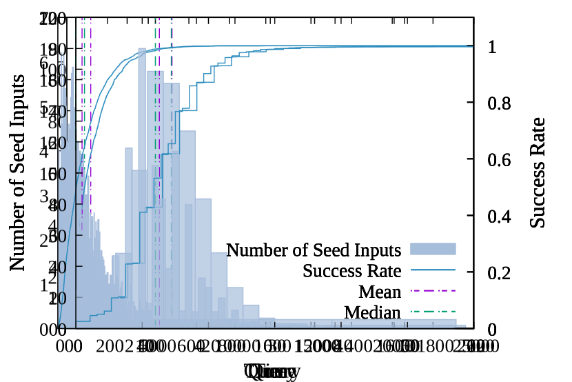
(c) DiffChaser, LeNet5 Quantization-8-bit

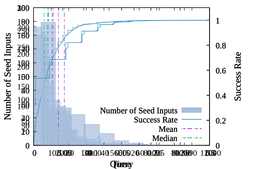
(d) DiffChaser, ResNet-20, Knowledge Distillation

Figure 4. Histogram of the number of queries required by Dflare and DiffChaser to find the triggering input for the given seed input. The value is averaged over five repeated experiments.

5.2. RQ2: Efficiency

5.2.1. Time

The two Average Time columns in Table 4 show the average time spent by Dflare and DiffChaser to find triggering inputs for each seed input if successful. The time needed by Dflare to find one triggering input ranges from 0.029s to 3.369s, with the average value 0.518s. DiffChaser takes much longer time than Dflare. Specifically, DiffChaser takes 10.654s$\sim$163.936s to find one triggering input, with the average 52.234s. On average, Dflare is 230.94x (17.84x$\sim$446.06x) as fast as DiffChaser in terms of time.

5.2.2. Query

The two Average Query columns in Table 4 show the average query issued by Dflare and DiffChaser for all seed inputs if a triggering input can be found. Generally, Dflare only needs less than 30 queries to find a triggering input, with only two exceptions. On average, Dflare requires only 24.99 queries (3.9$\sim$117.0). DiffChaser always needs thousands of queries for each trigger input (averagely 3642.50), much more than Dflare. For example, the smallest number of queries needed by DiffChaser is 1,896.59 for PlainNet-20 and its pruned model. In the same pair of models, Dflare only needs 4.31 queries on average. Overall, the number of queries required by Dflare is 0.699% (0.186%$\sim$1.937%) of the one required by DiffChaser.

We further visualize the queries of Dflare and DiffChaser in Figure 4 on two pairs of models: LeNet-5 Quantization-8-bit and ResNet-20 Knowledge Distillation. They are selected since the ratio of queries needed by Dflare over the one needed by DiffChaser is the smallest (0.186%) and largest (1.937%) in all the 21 pairs of models. Figure 4 shows the histogram of the number of queries needed by Dflare and DiffChaser, respectively, as well as the mean and median. It can be observed that Dflare significantly outperforms DiffChaser in terms of queries. The reason is that DiffChaser adopts a genetic algorithm to generate many inputs via crossover and feed them into DNN models in each iteration. As a result, it requires thousands of queries from the two models to find a triggering input. In contrast, Dflare only needs to generate one mutated input and query once in each iteration.

5.3. RQ3: Ablation Study

We further investigate the effects of our fitness function and mutation operator selection strategy. Specifically, we create the following two variants of Dflare.

1. $\text{{{Dflare}}}_{D}$: the fitness function in Dflare is replaced by a simpler fitness function: $H_{f,g}(x)=\mathcal{D}_{f,g}(x)=|p_{f(x)}-p_{g(x)}|$. In other words, the fitness function does not trace the model states triggered by inputs.

2. $\text{{{Dflare}}}_{R}$: the selection strategy for mutation operators in Dflare is changed to uniform random selection.

Table 6. Evaluation results of $\text{{{Dflare}}}_{D}$ and $\text{{{Dflare}}}_{R}$. The numbers in parentheses are the ratios of time or queries spent by each variant with respect the one spent by Dflare. The results are averaged across five runs using different random seeds.

Dataset	Model	Compression	$\text{{{Dflare}}}_{D}$			$\text{{{Dflare}}}_{R}$
			Average	Average	Average	Average	Average	Average
			Success	Time	Query	Success	Time	Query
			Rate	(sec)		Rate	(sec)
MNIST	LeNet-1	Quantization-8bit	41.44%	39.988 (77.93)	8140.54 (96.94)	100%	0.537 (1.05)	89.52 (1.07)
	LeNet-5	Quantization-8bit	39.44%	38.244 (54.15)	7422.38 (63.43)	100%	0.752 (1.07)	125.87 (1.08)
CIFAR-10	ResNet-20	Quantization-8bit	100%	3.454 (6.78)	203.91 (6.70)	100%	0.555 (1.09)	30.59 (1.01)
MNIST	LeNet-4	Prune	92.12%	8.242 (148.23)	2970.80 (161.98)	100%	0.062 (1.12)	20.79 (1.13)
		Quantization	60.76%	31.162 (166.55)	4861.92 (174.69)	100%	0.200 (1.07)	30.06 (1.08)
	LeNet-5	Prune	93.52%	7.428 (104.62)	2473.71 (112.27)	100%	0.080 (1.13)	24.77 (1.12)
		Quantization	59.92%	26.699 (118.72)	3548.56 (126.38)	100%	0.237 (1.05)	29.99 (1.07)
	CNN	Prune	81.04%	11.396 (168.58)	4348.22 (193.20)	100%	0.075 (1.11)	25.14 (1.12)
		Quantization	63.68%	26.639 (154.16)	4243.05 (167.46)	100%	0.182 (1.05)	26.39 (1.04)
CIFAR-10	PlainNet-20	Prune	100%	0.037 (1.28)	5.16 (1.30)	100%	0.031 (1.05)	4.05 (1.02)
		Quantization	100%	0.058 (1.14)	5.11 (1.18)	100%	0.051 (1.00)	4.32 (1.00)
		Knowledge Distillation	100%	0.809 (1.72)	15.85 (1.74)	100%	0.477 (1.02)	9.30 (1.02)
	ResNet-20	Prune	100%	0.039 (1.22)	4.95 (1.27)	100%	0.031 (0.98)	3.80 (0.97)
		Quantization	100%	0.080 (1.26)	6.07 (1.29)	100%	0.066 (1.03)	4.89 (1.04)
		Knowledge Distillation	100%	1.329 (1.94)	19.39 (1.91)	100%	0.690 (1.01)	10.07 (0.99)
	VGG-16	Prune	100%	0.047 (1.28)	7.86 (1.36)	100%	0.035 (0.95)	5.49 (0.95)
		Quantization	100%	0.050 (1.20)	7.48 (1.28)	100%	0.042 (1.01)	5.90 (1.01)
		Knowledge Distillation	99.04%	4.986 (4.22)	117.08 (4.48)	100%	1.133 (0.96)	24.75 (0.95)
ImageNet	Inception	Quantization	79.4%	16.064 (12.69)	251.55(11.73)	100%	1.459 (1.15)	25.01 (1.17)
	ResNet-50	Quantization	87.4%	12.789 (15.63)	253.57(13.18)	100%	1.418 (1.73)	20.34 (1.06)
	ResNeXt-101	Quantization	48.2%	29.019 (7.86)	277.17(8.04)	100%	4.240 (1.15)	40.64 (1.18)
Average Ratio w.r.t. Dflare				50.06	54.85		1.09	1.05

For each variant, we measure its success rate, computation time, and the number of queries needed using the seed inputs of the preceding experiments. Table 6 shows the results. The numbers in parentheses are the ratios of time or queries spent by each variant with respect the one(s) spent by Dflare.

5.3.1. Fitness Function

The column $\text{{{Dflare}}}_{D}$ in Table 6 shows the evaluation results of $\text{{{Dflare}}}_{D}$. Although $\text{{{Dflare}}}_{D}$ still achieves 100% success rate in half of the 21 model pairs, the success rates of $\text{{{Dflare}}}_{D}$ for the remaining 21 pairs are clearly lower than those of Dflare, ranging from 39.44% to 99.04%. The average success rate of $\text{{{Dflare}}}_{D}$ over all 21 pairs of models is only 83.14%. In terms of the computation time and the number of queries, $\text{{{Dflare}}}_{D}$ is much less efficient than Dflare. Specifically, the time spent by $\text{{{Dflare}}}_{D}$ is 1.140x$\sim$168.58x of that spent by Dflare, with an average value 50.06x. As for the number of queries needed, the ratios range from 1.18x to 193.20x, and the average ratio is 54.85x. This result indicates the importance of encouraging the mutated inputs to explore more model states as formulated by our fitness function.

5.3.2. Selection Strategy of Mutation Operator

The column $\text{{{Dflare}}}_{R}$ in Table 6 shows the evaluation results of $\text{{{Dflare}}}_{R}$. Same as Dflare, $\text{{{Dflare}}}_{R}$ achieves 100% success rate. In terms of efficiency, the average time spent by $\text{{{Dflare}}}_{R}$ is 1.09x (0.95x$\sim$1.73x) of that spent by Dflare. The ratio of queries required by $\text{{{Dflare}}}_{R}$ over those by Dflare is also 1.05x, ranging from 0.95x to 1.18x. In 17 out of 21 pairs, the time and queries required by Dflare are 91.33% of that required by $\text{{{Dflare}}}_{R}$. For the remaining 4 pairs, $\text{{{Dflare}}}_{R}$ is marginally (3.5%) more efficient than Dflare in terms of time and the number of queries. A possible reason is that with our fitness function, a triggering input for these four pairs can be found in just a few iterations. In such cases, the selection strategy of Dflare has not obtained enough samples to capture the knowledge of each mutation operator before the triggering input is found. Therefore, it is possible that $\text{{{Dflare}}}_{R}$, which adopts a random mutation strategy with our effective fitness function, can find the triggering inputs sooner.

To check whether Dflare statistically outperforms $\text{{{Dflare}}}_{R}$ in terms of time, we conduct Wilcoxon significant test (Wilcoxon, 1945) and the p-value is $3.604\times 10^{-4}$. The p-value indicates that our MH algorithm for mutation operator selection significantly improves the efficiency of finding triggering inputs.

5.4. Application of Dflare: Facilitating Model Dissemination

In this case study, we discuss a potential application of Dflare to facilitate model dissemination. Specifically, we are going to show that, to a certain extent, the time and number of queries taken to find triggering inputs can be leveraged as an approximation of to what extent the behavior of compressed models differs from that of the original models in the dissemination. Since Dflare can provide this metric effectively and efficiently, we argue that Dflare is able to provide developers with in-time feedback complementary to the accuracy metric, to assess compressed models.

5.4.1. Correlation

We would like to understand the correlation between the time and queries and to what extent the behavior of compressed models differs from that of the original models in deployment. We manually constructed a series of models from the original models LeNet-5, ResNet-20 and ResNet-50 in Table 2 by mutating $x\%$ of weights, where $x$ ranges from 10 to 50, with a step of 10. In the mutation, we randomly mutated the $x\%$ of the weights by increasing or decreasing their values by 10%. Intuitively, the larger $x$ is, the more likely the behavior of the resulted model differs from the one of original model. These models serve as a benchmark with the ground truth, i.e., to what extent the resulted model differs from the original one, for our study. Then we applied Dflare using the same experiment settings in section 4.4 and measured the time and number of queries.

(a) LeNet-5, MNIST

(b) ResNet-20, CIFAR-10

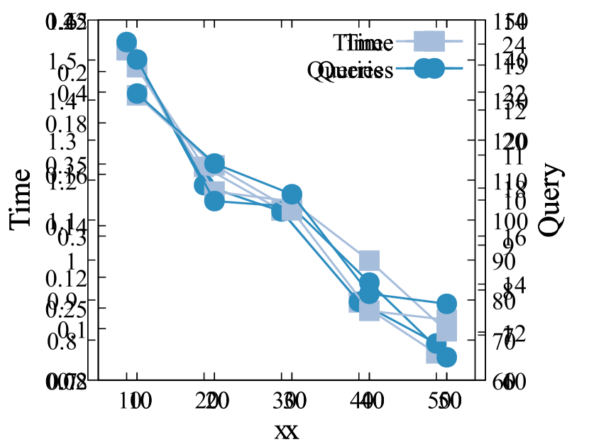
(c) ResNet-50, ImageNet

Figure 5. Correlation between time/query and mutation ratio $x$, using LeNet-5 for MNIST (Figure 5(a)), ResNet-20 for CIFAR-10 (Figure 5(b)), and ResNet-50 for ImageNet (Figure 5(c)).

Figures 5(a), 5(b) and 5(c) show the results for LeNet-5, ResNet-20, and ResNet-50, respectively. Success rates are not presented since all of them are 100%. It is clear that as the portion of the mutated weight $x$% increases, the time and queries required to find the triggering inputs decrease. The Pearson Correlation Coefficients (Benesty et al., 2009) between $x$ and time/queries also confirm this strong negative correlation, which are -0.989 (time) and -0.972 (queries) for LeNet-5, -0.968 and -0.967 for ResNet-20, and -0.979 and -0.977 for ResNet-50, respectively. Since the higher $x$ causes the resulted model to be more likely to differ from the original models, we claim that the time and queries can approximate to what extent the behavior of compressed models differs from the one of original models. Specifically, the less time and fewer queries needed to find triggering inputs, the more likely the compressed model differs from the original model in the dissemination.

5.4.2. Application

Now we present an application of Dflare in model dissemination. When compressing a pre-trained model, developers often need to prepare a compression configuration  (Li et al., 2017; Choudhary et al., 2020a). For example, the configuration of model pruning usually specifies which layers in the original model are to be pruned. A common way is to select the configuration that produces the highest accuracy on test set. However, as we will demonstrate, only using accuracy is insufficient to distinguish different models, and Dflare can provide complementary information to facilitate this process.

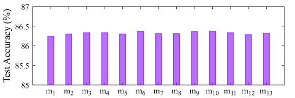
Figure 6. The test accuracy of thirteen compressed models.

We prepared a VGG-16 model by training it from scratch using the CIFAR-10 training dataset. After the loss and accuracy became saturated, its top-1 accuracy on the CIFAR-10 test set is 86.34%. Given this original model, we created a set of compressed models by pruning only one of the thirteen convolutional layers in the VGG-16 model at one time. In total, we collected thirteen compressed models using PyTorch and we referred to them as $m_{1}$, $m_{2}$, $\cdots$, $m_{13}$, where $m_{i}$ is the compressed model obtained by pruning the $i$-th convolutional layer of the original model. Figure 6 shows the top-1 accuracy of each compressed model. The accuracy of these models ranges from 86.24% to 86.37% and is almost identical to the accuracy of the original model (86.34%) with a maximal difference of 0.10%. If this developer uses accuracy as the single evaluation metric, it seems that these models achieve indistinguishable performance, and thus it makes no difference to select any of them for dissemination.

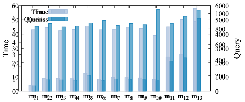
(a) Dflare

(b) DiffChaser

Figure 7. The results using Dflare and DiffChaser on thirteen compressed models.

In this scenario, Dflare can quickly provide complementary information that is orthogonal to accuracy. Figure 7(a) shows the average time and queries when using Dflare to find one bug-triggering input. Same as the previous settings, we repeated each experiment five times using 500 seed inputs. Although the accuracy of these models is similar, the information generated by Dflare leads to a different conclusion. Specifically, it is relatively harder to find a deviated behavior for the compressed model whose pruned layer is at the bottom of VGG-16, than the models whose pruned layer is at the top. For example, $m_{13}$ requires much more time and queries than $m_{1}$. According to the aforementioned correlation, if we use the time and number of queries as an approximation of the likelihood that the compressed model behaves differently from the original model, it is clear that $m_{13}$ has the least likelihood among all thirteen models. Taking account of the perspectives from both accuracy and this likelihood information provided by Dflare, the developers should choose the compressed model $m_{13}$ or $m_{12}$ for dissemination, since they have not only the comparable accuracy, but also the least likelihood to exhibit deviated behaviors.

Figure 7(b) shows the results generated by DiffChaser. The average success rate of DiffChaser is only 86.3%, which is 13.7% lower than Dflare. The time and number of queries required by DiffChaser demonstrate the same trend as the one using Dflare, i.e., the models whose pruned layers are at the bottom of the VGG16, e.g. $m_{13}$/$m_{12}$, are less likely to have deviated behaviors than others, e.g. $m_{1}$/$m_{2}$. Dflare can provide such in-time feedback to developers due to its high effectiveness and efficiency, making it practical to utilize this technique in daily tasks. In contrast, even though DiffChaser may also provide similar information, it takes much a longer time (37.4x on average) and more queries (29.74x) to do so, imposing large computation cost. For example, given a set of 500 seed inputs and $m_{2}$, DiffChaser requires 6.1 hours and 2,370,800 queries, while Dflare only needs 8.9 minutes and 73,320 queries.

5.5. Application of Dflare: Repairing the Deviated Behaviors

We further explored the possibility to repair the deviated behaviors of the compressed models for image classification models using the triggering inputs found by Dflare. A common approach to improving the performance of DNN models is to retrain the DNN models. For example, adversarial training can improve the robustness of DNN models (Zhang et al., 2019; Shafahi et al., 2019). However, without accessing the internal architectures and status of compressed models, it is difficult to repair the deviated behaviors directly via retraining. Therefore, we explored an alternative approach that repairs the deviated behaviors without the need to retrain the compressed model. Please note that we are not attempting to repair the triggering inputs in the original test sets, since the number of triggering inputs in the original test set is ineligible, as shown in Algorithm 2. It is the duty of compression techniques to reduce the number of triggering inputs in the original test set, to avoid accuracy degradation due to model compression.

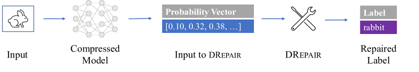
(a) Deployment Stage

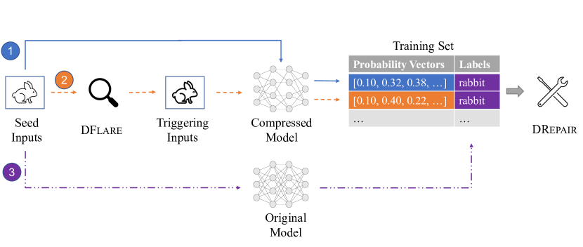
(b) Training Stage

Figure 8. The workflow of Drepair to repair deviated behaviors of compressed model.

5.5.1. Design of Drepair

We proposed a prototype, Drepair, to repair the deviated behaviors of the compressed models for image classifications. Our intuition is that the substantial amount of triggering inputs found by Dflare contains essential characteristics of such triggering inputs, and may thus be used to train a separate repair model to fix the deviated behaviors. Figure 8(a) illustrates the workflow of Drepair. Drepair is a supervised classifier, serving as a post-processing stage of the target compressed model. Given an input $x$ and the probability vector $g(x)=[p_{1},p_{2},p_{3},\cdots,p_{n}]$ outputted by a compressed model $g$, Drepair takes as input the probability vector $g(x)$ and is expected to output a label $\overline{l_{g(x)}}$ such that $\overline{l_{g(x)}}=l_{f(x)}$, where the label $l_{f(x)}$ is outputted by the original model $f$ given the same input $x$.

Figure 8(b) shows the workflow to train Drepair. After collecting a set of seed inputs, we first feed each seed input $x_{s}$ to the compressed model under test $g$ and collect the probability vector $g(x_{s})$. Then we utilize Dflare to find the triggering input $x_{t}$ given the seed input $x_{s}$ and obtain its probability vector $g(x_{t})$ using the compressed model $g$. Since Drepair is a supervised classifier, each vector in the training set is assigned a target label. For vector $g(x)$, we use the label outputted by the original model $f$ given input $x$ as the target label, i.e. $l_{f(x)}$. This is because the objective of Drepair is to produce a label that is the same as the label from original model.

5.5.2. Implementation and Evaluation of Drepair

We implemented Drepair using a Single-layer Perceptron (SLP), i.e., a neural network with a single hidden layer (Rumelhart et al., 1988). We chose SLP since it is light-weight in terms of computational resources and thus is applicable to be deployed along with compressed models in embedded systems. We used five-fold cross-validation to evaluate the performance of Drepair using the seed inputs and triggering inputs found by Dflare in RQ2. Specifically, for each set of 500 pairs of seed input and triggering input, we collected their probability vectors and split them into five portions of equal size. We chose four of them for the training set of Drepair, and the remaining one as its test set. In other words, each training set contains 400 non-triggering inputs and 400 triggering inputs, and each test set $X$ contains 100 non-triggering inputs and 100 triggering inputs. In a five-fold cross-validation, we repeated the training and testing five times and ensured a different training and test set is used in each time. Each five-fold cross-validation was conducted 5 times using different random seeds.

We measure the performance of Drepair from the following three perspectives. In particular, we use $X_{t}$ to denote the set of triggering input and use ${X_{s}}$ to denote non-triggering inputs in the test set $X$. As we mentioned in the above paragraph, the sizes of $X_{t}$, $X_{s}$ and $X$ are 100, 100 and 200, respectively.

Repair Count and Repair Ratio.  We first use Repair Count to measure the number of triggering inputs in $X_{t}$ that do not trigger deviated behaviors after repair, i.e.,

$$\text{Repair Count}=\sum_{i=1}^{|X_{t}|}{o_{x_{i}}}$$

where $o_{x_{i}}$ is an indicator and $o_{x_{i}}=1$ only if $\overline{l_{g(x_{i})}}=l_{f(x_{i})}$, i.e., $x_{i}$ does not trigger deviated behavior after repair; otherwise, it is 0. $|X_{t}|$ is the number of inputs in $X_{t}$.

We then measure Repair Ratio, i.e., the ratio of Repair Count in $X_{t}$. Repair Ratio measures the percentage of triggering inputs in $X_{t}$ that do not trigger deviated behaviors after repair. The higher the repair ratio is, the more triggering inputs are repaired by Drepair.

$$\text{Repair Ratio}=\frac{\text{Repair Count}}{|X_{t}|}\times 100\%=\frac{\sum_{i=1}^{|X_{t}|}{o_{x_{i}}}}{|X_{t}|}\times 100\%$$

Inducing Count and Inducing Ratio.  We use Inducing Count to denote the number of non-triggering inputs in $X_{s}$ that trigger deviated behaviors after repair, i.e.

$$\text{Inducing Count}=\sum_{i=1}^{|X_{s}|}{k_{x_{i}}}$$

where $k_{x_{i}}$ is an indicator and $k_{x_{i}}=1$ only if $\overline{l_{g(x_{i})}}\neq l_{f(x_{i})}$, i.e., $x_{i}$ triggers deviated behaviors after repair; otherwise, it is 0. $|X_{s}|$ is the number of inputs in $X_{s}$.

Then we use Inducing Ratio to measure the ratio of Inducing Count in $X_{s}$. Specifically, Inducing Ratio measure the percentage of non-triggering inputs in $X_{s}$ that trigger deviated behaviors after repair. The lower the inducing ratio is, the fewer deviated behaviors are induced by Drepair.

$$\text{Inducing Ratio}=\frac{\text{Inducing Count}}{|X_{s}|}=\frac{\sum_{i=1}^{|X_{s}|}{k_{x_{i}}}}{|X_{s}|}\times 100\%$$

Improvement Count and Improvement Ratio.  We use Improvement Count to measure the difference between the number of deviated behaviors in $X$ before repair by Drepair and the number of deviated behaviors in $X$ after repair. Specifically, the number of deviated behaviors before the repair is equal to the number of triggering inputs in $X$, i.e. $|X_{t}|$. A deviated behavior after repair is triggered by ${x_{i}}$ if $\overline{l_{g(x_{i})}}\neq l_{f(x_{i})}$. Since the indicator $k_{x_{i}}=1$ if and only if $\overline{l_{g(x_{i})}}\neq l_{f(x_{i})}$, the number of deviated behaviors after repair in $X$ is counted as $\sum_{i=1}^{|X|}{k_{x_{i}}}$. Therefore, the difference between the number of deviated behaviors in $X$ before repair and after repair is denoted as

$$\text{Improvement Count}=|X_{t}|-\sum_{i=1}^{|X|}{k_{x_{i}}}$$

We then use Improvement Ratio to measure the ratio of Improvement Count w.r.t. to the number of deviated behaviors in $X$ before repair. The higher the improvement ratio is, the more effective Drepair is to repair the deviated behaviors of compressed models.

$$\text{Improvement Ratio}=\frac{\text{Improvement Count}}{|X_{t}|}\times 100\%=\frac{|X_{t}|-\sum_{i=1}^{|X|}{k_{x_{i}}}}{|X_{t}|}\times 100\%$$

Noticed that the Improvement Ratio can be zero or negative when the number of triggering inputs after repair is equal to or larger than the number of triggering inputs before repair, i.e., $\text{Improvement Count}\leq 0$. In such situations, the repair process fails since the number of deviated behavior after repair is more than or equal to the number of deviated behavior before repair.

Table 7. Evaluation results of Drepair. The results are averaged across five-fold cross-validation. Noticed that since $X_{s}$ and $X_{t}$ are equal to 100 in each fold of validation, the $\text{Count}=\text{Ratio}\times 100$.

Dataset	Model	Compression	Drepair
			Average		Average		Average
			Repair		Inducing		Improvement
			Count	Ratio	Count	Ratio	Count	Ratio
MNIST	LeNet-1	Quantization-8-bit	30.56	30.56%	0.36	0.36%	30.20	30.20%
	LeNet-5	Quantization-8-bit	24.28	24.28%	0.12	0.12%	24.16	24.16%
CIFAR-10	ResNet-20	Quantization-8-bit	15.04	15.04%	0.52	0.52%	14.52	14.52%
MNIST	LeNet-4	Prune	48.48	48.48%	0.00	0.00%	48.48	48.48%
		Quantization	35.68	35.68%	0.00	0.00%	35.68	35.68%
	LeNet-5	Prune	43.20	43.20%	0.08	0.08%	43.12	43.12%
		Quantization	38.68	38.68%	0.00	0.00%	38.68	38.68%
	CNN	Prune	42.44	42.44%	0.04	0.04%	42.40	42.40%
		Quantization	36.55	36.55%	0.04	0.04%	36.50	36.50%
CIFAR-10	PlainNet-20	Prune	50.40	50.40%	12.92	12.92%	37.48	37.48%
		Quantization	32.20	32.20%	8.16	8.16%	24.04	24.04%
		Knowledge Distillation	23.34	23.34%	6.77	6.77%	16.56	16.56%
	ResNet-20	Prune	49.32	49.32%	12.24	12.24%	37.08	37.08%
		Quantization	36.28	36.28%	6.44	6.44%	29.84	29.84%
		Knowledge Distillation	24.78	24.78%	6.38	6.38%	18.40	18.40%
	VGG-16	Prune	37.68	37.68%	5.12	5.12%	32.56	32.56%
		Quantization	25.64	25.64%	6.88	6.88%	18.76	18.76%
		Knowledge Distillation	19.28	19.28%	4.78	4.78%	14.50	14.50%
ImageNet	Inception	Quantization	28.69	28.69%	7.26	7.26%	21.43	21.43%
	ResNet-50	Quantization	18.94	18.94%	4.01	4.01%	14.93	14.93%
	ResNeXt-101	Quantization	25.92	25.92%	5.44	5.44%	20.48	20.48%
Average			32.73	32.73%	4.17	4.17%	28.56	28.56%

Table 7 shows the results. On average, Drepair repairs 32.73% triggering inputs. Although Drepair induces 4.17% new deviated behaviors, overall Drepair reduces the number of deviated behaviors by 30.16%. In the best case, the number of deviated behaviors is reduced by 48.48%. In conclusion, it is feasible to repair the deviated behaviors using the triggering inputs found by Dflare. A promising feature work is to propose more advanced approaches to achieve this objective.

Table 8. The effectiveness and efficiency of Dflare on the compressed model without Drepair and with Drepair. The numbers in parentheses are the ratios of time or queries spent by Dflare on the compressed model repaired by Drepair with respect the one spent by Dflare on the model without Drepair. The results are averaged across five runs using different random seeds.

Dataset	Model	Compression		Without Drepair			With Drepair
			Improvement	Average	Average	Average	Average	Average	Average
			Ratio	Success	Time	Query	Success	Time	Query
				Rate	(sec)		Rate	(sec)
MNIST	LeNet-4	Prune	48.48%	100%	0.056	18.34	100%	0.245 (4.83)	55.67 (3.04)
	LeNet-5	Prune	43.12%	100%	0.071	22.03	100%	0.169 (2.38)	33.86 (1.54)
	CNN	Prune	42.40%	100%	0.068	22.51	100%	0.399 (5.87)	102.29 (4.54)
ImageNet	Inception	Quantization	21.44%	100%	1.266	21.44	100%	2.880 (2.27)	31.40 (1.46)
	ResNet-50	Quantization	18.94%	100%	0.819	19.24	100%	2.959 (3.61)	39.45 (2.05)
	ResNeXt-101	Quantization	25.92%	100%	3.693	34.49	100%	9.872 (2.67)	55.06 (1.60)

We further leveraged Dflare to test these models that are repaired by Drepair. Specifically, we selected the three models that have the highest improvement ratios to see if these models that are relatively successfully repaired by Drepair can decrease the effectiveness or efficiency Dflare. Meanwhile, we also selected the three models trained on ImageNet to investigate the effects of Drepair in large and complex models. Table 8 shows the effectiveness and efficiency of Dflare when the compressed model is not repaired by Drepair and when the compressed model is repaired by Drepair. After repair, Dflare can still achieve 100% success rates in these six models. However, the time spent by Dflare to find each triggering input in the compressed model repaired by Drepair is 2.27x$\sim$5.87x as the one spent by Dflare on the compressed models without repair. The number of queries is also increased to 1.46x$\sim$4.54x as the one without repair. As a proof of concept proposed by us, Drepair can effectively decrease the efficiency of Dflare. We will make the efforts to improve the effectiveness of Drepair as our following work.

6. Discussion and Future Work

6.1. Demonstration of the Generalizability of Dflare on Other Domain

Our study focuses on the compressed models for image classifications, but our approach can also be applied to the compressed models in other domains after proper adaptions, especially the mutation operators. To demonstrate this, we applied Dflare to the compressed models on Speech-to-Text task. Given an audio clip as input, Speech-to-Text models aim to translate the audio into text. We used the original models and compressed models provided by Mozilla DeepSpeech (Hannun et al., 2014). We selected Mozilla DeepSpeech since it is a well-recognized open-source project (with more than 20,000 stars) and it provides detailed documentation for us to deploy. There are two pairs of original models and compressed model used in our evaluation. Specifically, the latest version of DeepSpeech, i.e., v0.9.3, provides a pair of original model and compressed models and the second latest version, v0.8.2, provides the second pair of models (versions between these two versions provide the same models as v0.9.3). In both version, the compressed models are quantized from the original models.

We adjusted Dflare in two aspects to apply it in Speech-to-Text models. First, we adopted the audio-specific mutation operators since audio and images have different characteristics. Specifically, we used the operators TimeStretch, PitchShift, TimeShift, and Gain (volume adjustment) provided by Audiomentations, a Python library to mutate audio. Since these operators are also used in DeepSpeech for data augmentation during model training, we believe that these operators are regarded as representative mutations by developers. Second, since the output of Speech-to-Text models is a sentence, rather than a label in image classifications, we also adjusted the methodology to compare the outputs of original models and compressed models. Specifically, in image classification models, Dflare compares the labels outputted by original models and compressed models, while in Speech-to-Text, Dflare compares the sentences word by word. Given the same audio, if the original model and compressed model output different sentences, such as “the character which your royal highness assumed is imperfect harmony with your own” vs “the character which your royal highness summed is imperfect harmony with your own”, such an audio input is labeled as triggering input. We also made the same adjustment to the baseline DiffChaser. Three authors carefully reviewed the adjustment to avoid possible mistakes.

We randomly selected 500 audio inputs from the test set of Librispeech dataset (Panayotov et al., 2015). According to the documentation, Librispeech is used by Mozilla DeepSpeech in training and testing. We used the same timeout as RQ1, i.e., 180 seconds. The experiments were repeated five times using different random seeds.

Table 9. Effectiveness of Dflare on on Speech-to-Text models. The results are averaged across five runs.

Model	Version	Compression	Dflare			DiffChaser
			Average	Average	Average	Average	Average	Average
			Success	Time	Query	Success	Time	Query
			Rate	(sec)		Rate	(sec)
DeepSpeech	v0.9.3	Quantization	100%	5.740	8.42	95.6%	169.365	223.04
	v0.8.2	Quantization	100%	4.812	5.88	95.5%	168.402	214.53

Table 9 shows results. The success rates of Dflare are 100% in five runs. On average, it takes Dflare 4.812$\sim$5.740s and 5.88$\sim$8.42 queries to find a triggering input. By contrast, DiffChaser fails to find triggering inputs for around 4.5% seed inputs and it takes DiffChaser around 168 seconds and 214.53$\sim$223.04 queries to find one triggering input. The time and queries spent by Dflare is only 2.4%$\sim$3.4% and 2.7%$\sim$3.8% of the one required by DiffChaser, respectively. This result demonstrates the effectiveness and efficiency of Dflare on Speech-to-Text tasks.

We also tried to fix the triggering inputs using Drepair but we were not able to achieve a reasonable result. Our conjecture is that repairing the models trained for Speech-to-Task are much more complicated than the models trained for image classifications. Specifically, for image classification models trained on ImageNet, Drepair is expected to output the label that is same as the label outputted by the original model from 1,000 candidate labels (since ImageNet has 1,000 image labels). In contrast, for the Speech-to-Text task, the output of models is a sentence that can have an arbitrary number of words and there are around 977,000 unique English words in Librispeech. To successfully repair the results outputted by compressed models, Drepair needs to not only select a correct set of words from these 977,000 words, but also make sure these words are in the proper order since the meaning of a sentence also depends on the order of words. As a simple prototype proposed by us, Drepair is not able to handle such a complicated scenario. We leave the improvement of Drepair of large datasets like Librispeech for future work.

6.2. Effect of Timeout

In our evaluation, we used 180s as timeout for both Dflare and DiffChaser. To understand the effect of timeout on the effectiveness of Dflare, we conducted further experiments using smaller timeouts. Specifically, we evaluated the success rate of Dflare using 15s, 10s and 5s. Our experiments covered all the pairs of models in RQ2 and used all the images from MNIST and CIFAR-10 test sets as seed inputs.

Dflare achieves 100% success rates for the 14 pairs of models out of 21 pairs even using 5s as the timeout. Table 10 shows the results of the remaining four pairs of models. The success rates of Dflare for these four pairs drop to different levels when the timeout is shortened. The most significant decrease comes from the PlainNet-20 and its quantized model. Specifically, its success rate drops to 76.93% when the timeout is set to 15s. The success rate drops further to 10.90% with 5s timeout. The success rate for VGG-16 and its compressed model also drops to 40.06% with 5s timeout. As for the other two pairs of models in Table 10, their success rates slightly decrease to 99.98% and 89.12% if 5s timeout is used, respectively. In summary, Dflare is effective for 16 out of 21 pairs of models even a short timeout such as 10s is used.

An interesting observation from Table 10 is that all the compressed models in  Table 10 are compressed using 8-bit quantization. A possible explanation is that the difference between an original model and its compressed model induced by quantization is relatively smaller than the difference induced by pruning and knowledge distillation. Therefore, it takes a relatively long time for Dflare to find the deviated behavior for quantized models.

Table 10. The success rates of Dflare using different timeouts. The pairs of models that have 100% success rate using 5s timeout are not included. The results are averaged across five runs.

Dataset	Model	Compression	Timeout
			15s	10s	5s
CIFAR-10	ResNet-20	Quantization-8-bit	100%	100%	99.98%
CIFAR-10	PlainNet-20	Quantization	76.93%	43.76%	10.90%
	ResNet-20	Quantization	100%	99.30%	89.12%
	VGG-16	Quantization	95.87%	79.30%	40.06%

6.3. Uniqueness of Triggering Inputs

We carefully checked the triggering inputs found by Dflare in Table 4. Specifically, we first represented each triggering input $x$ as a matrix $A_{x}$ with size $H\times W\times C$, where $H$ and $W$ are the height and width of the image, respectively, and $C$ refers to the number of channels of the image ($C=3$ in color images and $C=1$ in gray images). Please note that the pixels in images are integers in the range $\left[0,255\right]$, and thus the elements in $A_{x}$ are also integer numbers in the range $\left[0,255\right]$. For each triggering input $x$, we check if there exists a triggering input $y$ such that the matrix $A_{x}$ is equal to the matrix $A_{y}$. If such $y$ exists, the inputs $x$ and $y$ are labeled as duplicated triggering inputs. Otherwise, $x$ is a unique triggering input.

Out of 105 experiments (21 pairs of models $\times$ 5 runs), 77 experiments do not have any duplicated triggering inputs. For the remaining 28 experiments, on average, 99.04% of the triggering inputs are unique to each other. In other words, the vast majority of the triggering inputs found by Dflare are unique.

6.4. Future Work

A useful future work is to fix the deviated behaviors for compressed DNN models. As we showed in section 5.5, there is still a significant improvement space for the performance of our repair prototype. A promising research direction is to propose an effective and efficient approach for this issue.

In section 6.1, we demonstrate the generalizability of Dflare in Speech-to-Text tasks. A promising direction is to apply Dflare to other domains, such as natural language process (Devlin et al., 2018) and object detection (Ren et al., 2017). To achieve this, the mutation operators should be properly customized based on domain-specific knowledge. Meanwhile, the test oracle may be adjusted accordingly, since the DNN models in other domains may concern factors other than labels. For example, in object detection, the location and boundary of the detected object are also important (Hosang et al., 2015). Moreover, a sufficient number of compressed models and datasets from the AI community are critical to comprehensively evaluate the new techniques in other domains. We believe it is a fruitful working direction to explore.

Another potential follow-up direction is to leverage Dflare to directly test the DNN models deployed on the embedded or mobile platforms. This may help the developers reveal the deviated behaviors induced by the hardware or firmware of such platforms.

7. Threats to Validity

7.1. Internal Threats

First, both Dflare and DiffChaser have randomness at certain levels. Such randomness may affect the evaluation results. To alleviate this, all experiments are repeated five times using different random seeds and the average results are presented. We found that the variance across these five runs are low and the conclusions of our evaluation are consistent in each run, i.e., Dflare outperforms DiffChaser in both effectiveness and efficiency. Therefore, we did not run the experiments more times.

Second, to comprehensively evaluate Dflare using diverse compressed DNN models, we construct the first benchmark containing 21 pairs of original model and its compressed model. Since there are no published pairs of the original model and its compressed model for 15 out of 21 pairs, we prepare them based on popular compression algorithms. Specifically, we train the DNN models from scratch and then compress them using popular model compression techniques. Both processes may be affected by the randomness in deep learning at a certain level (Pham et al., 2020). To mitigate this threat, for model training, we follow the practice from AI community and train each model until the loss value is saturated. We also compare their accuracy with the one reported by their original publications. The accuracy of each model trained by us is close to its published accuracy. In order to make sure that the model compressed by us are valid evaluation subjects, we utilize an existing tool from Intel AI Lab (Zmora et al., 2019) and carefully follow the instructions. The accuracy of each compressed model is close to that of its original model. This suggests that our compression processes are reliable.

Third, it is possible that the triggering inputs found by Dflare do not comply with the real world data distribution. To alleviate such a problem, Dflare used the mutation operators from prior work (Pei et al., 2017; Xie et al., 2019b; Tian et al., 2018; Ma et al., 2018a; Xie et al., 2019a) and these mutation operators are designed to simulate the scenario that DNN models are likely to face in the real world. For example, the mutation operator Random Pixel Change simulates effects of “dirt on camera lens” (Pei et al., 2017). Gaussian Noise is one of the most frequently occurring noises in image signal (Boncelet, 2009). Therefore, the triggering inputs found by Dflare using these mutation operators are highly likely to comply with the real-world inputs to be fed to DNN models in model deployment.

Lastly, since the implementation of DiffChaser shared by its authors only supports image classification models, we carefully revised its source code to support Speech-to-Text models in section 6.1. It is possible that our revision might have mistakes and thus affects its effectiveness and efficiency. To address this threat, three authors carefully reviewed the changes made by us to avoid possible mistakes.

7.2. External Threats

We evaluate our approach using 21 compressed models. The selection may not cover all compression techniques proposed by the communities. To mitigate this, the models selected are representative as they are trained on two common datasets at different scales, and then compressed using popular model compression techniques. Besides, the architectures of the selected models are diverse and include the ones that are commonly used by existing studies (Pei et al., 2017; Tian et al., 2018, 2021).

8. Related Work

8.1. DNN Model Testing

DeepXplore (Pei et al., 2017) is the first technique targeted at testing DNN models. It proposed neuron coverage, which measures the activation state of neurons, to guide the generation of test inputs. DeepXplore is based on differential testing and it uses multiple models of a task to detect potential defects. To alleviate the need of multiple models under test, DeepTest (Tian et al., 2018) leverages metamorphic relations (Chen et al., 1998) that are expected to hold by a model as its test oracles. Both DeepXplore and DeepTest perturb their test inputs based on the gradient of deep learning models. TensorFuzz (Odena et al., 2019) and DeepHunter (Xie et al., 2019a) are whitebox fuzzing-based testing techniques. They guide the input mutation by certain predefined coverage, instead of gradient, in order to trigger the unexpected behaviors of deep learning models, e.g. numerical errors and classifications. To assess the quality of DNN models, DeepJanus (Riccio and Tonella, 2020) proposes the notion of frontier of behaviors, i.e., pairs of inputs that have different predictions from the same DNN model. Given a DNN model under test, DeepJanus leverages a multi-objective evolutionary approach to find the frontier of behaviors. It further utilizes the model-based input representation to assure the realism of generated inputs.

Our approach, Dflare, differs from these techniques in two ways. First, Dflare focuses on the deviated behaviors of compressed models, while existing techniques target the normal models. Second, the majority of existing testing techniques for DNN models are whitebox (Pei et al., 2017; Tian et al., 2018; Chen et al., 1998; Odena et al., 2019; Xie et al., 2019a), making use of the models’ internal states, such as gradients and neuron coverage, which are often unavailable for compressed models. Therefore, these techniques are not applicable to testing compressed DNN models. In contrast, our approach is specifically designed for compressed models and it does not require the internal information from the model under test. The black-box testing approaches, e.g., DeepJanus, with proper adaptations, are promising to be applied in finding deviated behaviors of compressed DNN models. We will explore this direction in the future work.

Besides DiffChaser, there are also several recent studies specifically targeting on compressed models. DiverGet (Yahmed et al., 2022) presents a search-based approach to assess quantization models for hyperspectral images. It proposes a set of domain-specific metamorphic relations to transform the hyperspectral images and use them to mutate hyperspectral images. BET (Wang et al., 2022b) is a testing method for convolutional neural network(CNN)s. It splits a convolutional kernel into multiple zones of which the weights have the same positive or negative signs. The insight is that the decisions of CNNs are likely to be affected by continuous perturbations, i.e., the perturbations that have the same sign with each zone. These two approaches are either specific to the compression methods (quantization model in DiverGet) or types of DNN (CNN in BET), while Dflare is a general approach for diverse types of model architectures and compression methods. We do not include their approach in our evaluation since their tools are not available.

8.2. Empirical Study on DNN Model Deployment Issues

Researchers have conducted several empirical studies to characterize the issues in deploying DNN models, including compressed DNN models. Guo et al. found that the DNN models deployed in other platforms may exhibit different behaviors from the original models (Guo et al., 2019a). Hu et al. conducted a deep analysis for quantization models (Hu et al., 2022). They found that retraining the compressed models with triggering inputs cannot effectively reduce the behavioral difference between the original model and the compressed one. Our approach, Dflare, is a testing technique for compressed models, with the aim to help developers address these issues in model deployment and dissemination. Using the triggering inputs found by Dflare, our prototype Drepair is able to repair up to 48.48% deviated behaviors.

8.3. Differential Testing

Dflare aims to find deviated behavior between two DNN models. Related works also include those applying differential testing to detect inconsistencies across two pieces of traditional software. McKeeman (McKeeman, 1998) originally proposed differential testing in 1998 to expose bugs in software systems using test cases that result in inconsistent execution results in multiple comparable systems. Le et al. (Le et al., 2014) introduced EMI, which applies differential testing on compilers using semantically equivalent programs. Inconsistent execution outputs of compiled programs may indicate defects in compilers. Further, differential testing is also applied in JVM implementations (Lindholm et al., 2014) using mutated Java bytecode (Chen et al., 2019).

The objective of Dflare is similar to differential testing. Rather than two pieces of code, the systems under test for Dflare are DNN models and their compressed ones.

8.4. Differential Verification of DNN models

ReluDiff (Paulsen et al., 2020a) and its following work (Paulsen et al., 2020b) share certain similar objectives with our approach although it is not a testing technique. It leverages the structural and behavioral similarities of the two closely related networks in parallel, to verify whether the output difference of the two models are within the specification. In the evaluation, they use the pairs of compressed model and the original model as subjects.

Our work differs from ReluDiff in two ways. First, ReluDiff can only be used in forward neural networks with relu activation function for both compressed and original models. This limits its application scenarios. Sophisticated DNN models usually contain convolutional layers and recurrent layers. The advantage of Dflare is that it makes no assumption on the model architecture, making it applicable to a wide range of application scenarios. Second, ReluDiff needs to know the architectures and weights of DNN models for verification, while Dflare works for black-box models.

9. Conclusion

We proposed Dflare, a novel, effective input generation method to find deviated behaviors between an original DNN model and its compressed model. Specifically, Dflare leverages the MH algorithm in the selection of a mutation operator at each iteration to successively mutate a given seed input. Dflare incorporates a novel fitness function to determine whether to use a mutated input in subsequent iterations. The results show that Dflare outperforms prior work in terms of both effectiveness and efficiency. Dflare constantly achieves 100% success rate but uses significantly less amount of time and queries than the state of the art. We also explored the possibility to repair such deviated behaviors using the triggering inputs found by Dflare. Our prototype Drepair can repair up to 48.48% deviated behaviors and decrease the effectiveness of Dflare on the repaired models.

- (1)
- Akhtar and Mian (2018) N. Akhtar and A. Mian. 2018. Threat of Adversarial Attacks on Deep Learning in Computer Vision: A Survey. IEEE Access 6 (2018), 14410–14430.
- Benesty et al. (2009) Jacob Benesty, Jingdong Chen, Yiteng Huang, and Israel Cohen. 2009. Pearson correlation coefficient. In Noise reduction in speech processing. Springer, 1–4.
- Bhagoji et al. (2018) Arjun Nitin Bhagoji, Warren He, Bo Li, and Dawn Song. 2018. Practical Black-Box Attacks on Deep Neural Networks Using Efficient Query Mechanisms. In ECCV 2018, Munich, Germany, September 8-14, 2018, Vol. 11216. Springer, 158–174.
- Boncelet (2009) Charles Boncelet. 2009. Chapter 7 - Image Noise Models. In The Essential Guide to Image Processing, Al Bovik (Ed.). Academic Press, Boston, 143–167. https://doi.org/10.1016/B978-0-12-374457-9.00007-X
- Buciluundefined et al. (2006) Cristian Buciluundefined, Rich Caruana, and Alexandru Niculescu-Mizil. 2006. Model Compression (KDD ’06). Association for Computing Machinery, New York, NY, USA, 535–541. https://doi.org/10.1145/1150402.1150464
- Cai et al. (2020) Han Cai, Chuang Gan, Tianzhe Wang, Zhekai Zhang, and Song Han. 2020. Once-for-All: Train One Network and Specialize it for Efficient Deployment. In 8th International Conference on Learning Representations, ICLR 2020, Addis Ababa, Ethiopia, April 26-30, 2020. OpenReview.net. https://openreview.net/forum?id=HylxE1HKwS
- Carlini and Wagner (2017) Nicholas Carlini and David A. Wagner. 2017. Towards Evaluating the Robustness of Neural Networks. In SP 2017, San Jose, CA, USA, May 22-26, 2017. IEEE Computer Society, 39–57.
- Chamain et al. (2022) Lahiru D. Chamain, Siyu Qi, and Zhi Ding. 2022. End-to-End Image Classification and Compression With Variational Autoencoders. IEEE Internet of Things Journal 9, 21 (2022), 21916–21931. https://doi.org/10.1109/JIOT.2022.3182313
- Chen et al. (1998) Tsong Yueh Chen, Shing-Chi Cheung, and Siu Ming Yiu. 1998. Metamorphic testing: a new approach for generating next test cases. Technical Report HKUST-CS98-01. Department of Computer Science, HKUST, Hong Kong.
- Chen et al. (2019) Yuting Chen, Ting Su, and Zhendong Su. 2019. Deep differential testing of JVM implementations. In ICSE 2019, Montreal, QC, Canada, May 25-31, 2019. IEEE / ACM, 1257–1268.
- Chen et al. (2016) Yuting Chen, Ting Su, Chengnian Sun, Zhendong Su, and Jianjun Zhao. 2016. Coverage-Directed Differential Testing of JVM Implementations. In PLDI ’16 (Santa Barbara, CA, USA). ACM, New York, NY, USA, 85–99.
- Chen et al. (2021) Zuohui Chen, RenXuan Wang, Yao Lu, jingyang Xiang, and Qi Xuan. 2021. Adversarial Sample Detection via Channel Pruning. In ICML 2021 Workshop on Adversarial Machine Learning. https://openreview.net/forum?id=MKfq7TuRBCK
- Cheng et al. (2019) Minhao Cheng, Thong Le, Pin-Yu Chen, Huan Zhang, Jinfeng Yi, and Cho-Jui Hsieh. 2019. Query-Efficient Hard-label Black-box Attack: An Optimization-based Approach. In ICLR 2019, New Orleans, LA, USA, May 6-9, 2019.
- Cho and Hariharan (2019) Jang Hyun Cho and Bharath Hariharan. 2019. On the Efficacy of Knowledge Distillation. In 2019 IEEE/CVF International Conference on Computer Vision (ICCV). 4793–4801. https://doi.org/10.1109/ICCV.2019.00489
- Choudhary et al. (2020a) Tejalal Choudhary, Vipul Mishra, Anurag Goswami, and Jagannathan Sarangapani. 2020a. A comprehensive survey on model compression and acceleration. Artificial Intelligence Review (08 Feb 2020).
- Choudhary et al. (2020b) Tejalal Choudhary, Vipul Mishra, Anurag Goswami, and Jagannathan Sarangapani. 2020b. A Comprehensive Survey on Model Compression and Acceleration. Artif. Intell. Rev. 53, 7 (oct 2020), 5113–5155. https://doi.org/10.1007/s10462-020-09816-7
- Deng et al. (2009) J. Deng, W. Dong, R. Socher, L.-J. Li, K. Li, and L. Fei-Fei. 2009. ImageNet: A Large-Scale Hierarchical Image Database. In CVPR09.
- Devlin et al. (2018) Jacob Devlin, Ming-Wei Chang, Kenton Lee, and Kristina Toutanova. 2018. BERT: Pre-training of Deep Bidirectional Transformers for Language Understanding. arXiv preprint arXiv:1810.04805 (2018).
- Gonzalez and Woods (2008) Rafael C. Gonzalez and Richard E. Woods. 2008. Digital image processing. Prentice Hall, Upper Saddle River, N.J. http://www.amazon.com/Digital-Image-Processing-3rd-Edition/dp/013168728X
- Goodfellow et al. (2015) Ian J. Goodfellow, Jonathon Shlens, and Christian Szegedy. 2015. Explaining and Harnessing Adversarial Examples. In ICLR 2015, San Diego, CA, USA, May 7-9, 2015, Conference Track Proceedings.
- Gou et al. (2021) Jianping Gou, Baosheng Yu, Stephen J. Maybank, and Dacheng Tao. 2021. Knowledge Distillation: A Survey. International Journal of Computer Vision 129, 6 (mar 2021), 1789–1819. https://doi.org/10.1007/s11263-021-01453-z
- Guo et al. (2019b) Chuan Guo, Jacob R. Gardner, Yurong You, Andrew Gordon Wilson, and Kilian Q. Weinberger. 2019b. Simple Black-box Adversarial Attacks. In ICML 2019, 9-15 June 2019, Long Beach, California, USA, Vol. 97. PMLR, 2484–2493.
- Guo et al. (2019a) Qianyu Guo, Sen Chen, Xiaofei Xie, Lei Ma, Qiang Hu, Hongtao Liu, Yang Liu, Jianjun Zhao, and Xiaohong Li. 2019a. An Empirical Study Towards Characterizing Deep Learning Development and Deployment Across Different Frameworks and Platforms. In 2019 34th IEEE/ACM International Conference on Automated Software Engineering (ASE). 810–822. https://doi.org/10.1109/ASE.2019.00080
- Han et al. (2016) Song Han, Huizi Mao, and William J. Dally. 2016. Deep Compression: Compressing Deep Neural Network with Pruning, Trained Quantization and Huffman Coding. In 4th International Conference on Learning Representations, ICLR 2016, San Juan, Puerto Rico, May 2-4, 2016, Conference Track Proceedings, Yoshua Bengio and Yann LeCun (Eds.). http://arxiv.org/abs/1510.00149
- Han et al. (2015) Song Han, Jeff Pool, John Tran, and William J. Dally. 2015. Learning Both Weights and Connections for Efficient Neural Networks. In NIPS’15 (Montreal, Canada). MIT Press, Cambridge, MA, USA, 1135–1143.
- Hannun et al. (2014) Awni Y. Hannun, Carl Case, Jared Casper, Bryan Catanzaro, Greg Diamos, Erich Elsen, Ryan Prenger, Sanjeev Satheesh, Shubho Sengupta, Adam Coates, and Andrew Y. Ng. 2014. Deep Speech: Scaling up end-to-end speech recognition. CoRR abs/1412.5567 (2014). arXiv:1412.5567 http://arxiv.org/abs/1412.5567
- Hosang et al. (2015) Jan Hendrik Hosang, Rodrigo Benenson, Piotr Dollár, and Bernt Schiele. 2015. What makes for effective detection proposals? CoRR abs/1502.05082 (2015). arXiv:1502.05082 http://arxiv.org/abs/1502.05082
- Hu et al. (2022) Qiang Hu, Yuejun Guo, Maxime Cordy, Xiaofei Xie, Wei Ma, Mike Papadakis, and Yves Le Traon. 2022. Characterizing and Understanding the Behavior of Quantized Models for Reliable Deployment. CoRR abs/2204.04220 (2022). https://doi.org/10.48550/arXiv.2204.04220 arXiv:2204.04220
- Huang et al. (2019) Kun Huang, Bingbing Ni, and Xiaokang Yang. 2019. Efficient Quantization for Neural Networks with Binary Weights and Low Bitwidth Activations. In Proceedings of the Thirty-Third AAAI Conference on Artificial Intelligence and Thirty-First Innovative Applications of Artificial Intelligence Conference and Ninth AAAI Symposium on Educational Advances in Artificial Intelligence (Honolulu, Hawaii, USA) (AAAI’19/IAAI’19/EAAI’19). AAAI Press, Article 473, 8 pages. https://doi.org/10.1609/aaai.v33i01.33013854
- Kass et al. (1998) Robert E. Kass, Bradley P. Carlin, Andrew Gelman, and Radford M. Neal. 1998. Markov chain monte carlo in practice: A roundtable discussion. American Statistician 52, 2 (May 1998), 93–100.
- Khalid et al. (2019) Faiq Khalid, Hassan Ali, Hammad Tariq, Muhammad Abdullah Hanif, Semeen Rehman, Rehan Ahmed, and Muhammad Shafique. 2019. QuSecNets: Quantization-based Defense Mechanism for Securing Deep Neural Network against Adversarial Attacks. In 2019 IEEE 25th International Symposium on On-Line Testing and Robust System Design (IOLTS). 182–187. https://doi.org/10.1109/IOLTS.2019.8854377
- Kim et al. (2019) Jinhan Kim, Robert Feldt, and Shin Yoo. 2019. Guiding Deep Learning System Testing Using Surprise Adequacy. In ICSE ’19 (Montreal, Quebec, Canada). IEEE Press, 1039–1049.
- Krizhevsky et al. (2009) Alex Krizhevsky, Vinod Nair, and Geoffrey Hinton. 2009. The CIFAR-10 dataset. (2009). http://www.cs.toronto.edu/~kriz/cifar.html
- Le et al. (2014) Vu Le, Mehrdad Afshari, and Zhendong Su. 2014. Compiler validation via equivalence modulo inputs. In PLDI ’14, Edinburgh, United Kingdom - June 09 - 11, 2014. ACM, 216–226.
- Le et al. (2015) Vu Le, Chengnian Sun, and Zhendong Su. 2015. Finding Deep Compiler Bugs via Guided Stochastic Program Mutation (OOPSLA 2015). ACM, New York, NY, USA, 386–399.
- Lecun et al. (1998) Yann Lecun, Léon Bottou, Yoshua Bengio, and Patrick Haffner. 1998. Gradient-based learning applied to document recognition. In Proceedings of the IEEE. 2278–2324.
- LeCun and Cortes (2010) Yann LeCun and Corinna Cortes. 2010. MNIST handwritten digit database. http://yann.lecun.com/exdb/mnist/. (2010). http://yann.lecun.com/exdb/mnist/
- Li et al. (2017) Hao Li, Asim Kadav, Igor Durdanovic, Hanan Samet, and Hans Peter Graf. 2017. Pruning Filters for Efficient ConvNets. In ICLR 2017, Toulon, France, April 24-26, 2017.
- Lin et al. (2020) Tao Lin, Sebastian U. Stich, Luis Barba, Daniil Dmitriev, and Martin Jaggi. 2020. Dynamic Model Pruning with Feedback. In 8th International Conference on Learning Representations, ICLR 2020, Addis Ababa, Ethiopia, April 26-30, 2020. OpenReview.net. https://openreview.net/forum?id=SJem8lSFwB
- Lindholm et al. (2014) Tim Lindholm, Frank Yellin, Gilad Bracha, and Alex Buckley. 2014. The Java Virtual Machine Specification, Java SE 8 Edition (1st ed.). Addison-Wesley Professional.
- Lite (2022) TensorFlow Lite. 2022. TensorFlow Lite. Retrieved May 20, 2022 from https://www.tensorflow.org/lite
- Liu et al. (2022) Jing Liu, Bohan Zhuang, Zhuangwei Zhuang, Yong Guo, Junzhou Huang, Jinhui Zhu, and Mingkui Tan. 2022. Discrimination-Aware Network Pruning for Deep Model Compression. IEEE Transactions on Pattern Analysis and Machine Intelligence 44, 8 (2022), 4035–4051. https://doi.org/10.1109/TPAMI.2021.3066410
- Liu et al. (2018) Qi Liu, Tao Liu, Zihao Liu, Yanzhi Wang, Yier Jin, and Wujie Wen. 2018. Security Analysis and Enhancement of Model Compressed Deep Learning Systems under Adversarial Attacks. In ASPDAC ’18 (Jeju, Republic of Korea). IEEE Press, 721–726.
- Ma et al. (2018a) Lei Ma, Felix Juefei-Xu, Fuyuan Zhang, Jiyuan Sun, Minhui Xue, Bo Li, Chunyang Chen, Ting Su, Li Li, Yang Liu, Jianjun Zhao, and Yadong Wang. 2018a. DeepGauge: Multi-granularity Testing Criteria for Deep Learning Systems. In ASE 2018 (Montpellier, France). ACM, New York, NY, USA, 120–131.
- Ma et al. (2018b) Lei Ma, Fuyuan Zhang, Jiyuan Sun, Minhui Xue, Bo Li, Felix Juefei-Xu, Chao Xie, Li Li, Yang Liu, Jianjun Zhao, and Yadong Wang. 2018b. DeepMutation: Mutation Testing of Deep Learning Systems. In ISSRE 2018, Memphis, TN, USA, October 15-18, 2018, Sudipto Ghosh, Roberto Natella, Bojan Cukic, Robin Poston, and Nuno Laranjeiro (Eds.). IEEE Computer Society, 100–111. https://ieeexplore.ieee.org/xpl/conhome/8536838/proceeding
- McKeeman (1998) William M. McKeeman. 1998. Differential Testing for Software. Digital Technical Journal 10, 1 (1998), 100–107.
- Meyn and Tweedie (2009) Sean Meyn and Richard L. Tweedie. 2009. Markov Chains and Stochastic Stability (2nd ed.). Cambridge University Press, USA.
- Mishra and Marr (2018) Asit K. Mishra and Debbie Marr. 2018. Apprentice: Using Knowledge Distillation Techniques To Improve Low-Precision Network Accuracy. In ICLR 2018, Vancouver, BC, Canada, April 30 - May 3, 2018.
- Muja and Lowe (2014) Marius Muja and David G. Lowe. 2014. Scalable Nearest Neighbor Algorithms for High Dimensional Data. IEEE Transactions on Pattern Analysis and Machine Intelligence 36, 11 (2014), 2227–2240.
- Odena et al. (2019) Augustus Odena, Catherine Olsson, David Andersen, and Ian J. Goodfellow. 2019. TensorFuzz: Debugging Neural Networks with Coverage-Guided Fuzzing. In ICML 2019, 9-15 June 2019, Long Beach, California, USA. 4901–4911.
- ONNX (2022) ONNX. 2022. ONNX Inference. Retrieved May 20, 2022 from https://onnxruntime.ai/
- Panayotov et al. (2015) Vassil Panayotov, Guoguo Chen, Daniel Povey, and Sanjeev Khudanpur. 2015. Librispeech: An ASR corpus based on public domain audio books. In 2015 IEEE International Conference on Acoustics, Speech and Signal Processing (ICASSP). 5206–5210. https://doi.org/10.1109/ICASSP.2015.7178964
- Paulsen et al. (2020a) Brandon Paulsen, Jingbo Wang, and Chao Wang. 2020a. ReluDiff: Differential Verification of Deep Neural Networks.. In ICSE ’20 (Seoul, Republic of Korea). ACM, New York, NY, USA, 714–726.
- Paulsen et al. (2020b) Brandon Paulsen, Jingbo Wang, Jiawei Wang, and Chao Wang. 2020b. NeuroDiff: Scalable Differential Verification of Neural Networks Using Fine-Grained Approximation. In ASE ’20. ACM, New York, NY, USA, 784–796.
- Pei et al. (2017) Kexin Pei, Yinzhi Cao, Junfeng Yang, and Suman Jana. 2017. DeepXplore: Automated Whitebox Testing of Deep Learning Systems. In SOSP ’17 (Shanghai, China). ACM, New York, NY, USA, 1–18.
- Pham et al. (2020) Hung Viet Pham, Shangshu Qian, Jiannan Wang, Thibaud Lutellier, Jonathan Rosenthal, Lin Tan, Yaoliang Yu, and Nachiappan Nagappan. 2020. Problems and Opportunities in Training Deep Learning Software Systems: An Analysis of Variance. In Proceedings of the 35th IEEE/ACM International Conference on Automated Software Engineering (Virtual Event, Australia) (ASE ’20). Association for Computing Machinery, New York, NY, USA, 771–783. https://doi.org/10.1145/3324884.3416545
- Polino et al. (2018) Antonio Polino, Razvan Pascanu, and Dan Alistarh. 2018. Model compression via distillation and quantization. In ICLR 2018, Vancouver, BC, Canada, April 30 - May 3, 2018, Conference Track Proceedings.
- PyTorch (2022) PyTorch. 2022. Models and pre-trained weights: Quantized models. Retrieved 2022-08-19 from https://pytorch.org/vision/stable/models.html#quantized-models
- Rastegari et al. (2016) Mohammad Rastegari, Vicente Ordonez, Joseph Redmon, and Ali Farhadi. 2016. XNOR-Net: ImageNet Classification Using Binary Convolutional Neural Networks. In ECCV 2016, Amsterdam, The Netherlands, October 11-14, 2016.
- Ren et al. (2017) S. Ren, K. He, R. Girshick, and J. Sun. 2017. Faster R-CNN: Towards Real-Time Object Detection with Region Proposal Networks. IEEE Transactions on Pattern Analysis and Machine Intelligence 39, 6 (June 2017), 1137–1149. https://doi.org/10.1109/TPAMI.2016.2577031
- Riccio and Tonella (2020) Vincenzo Riccio and Paolo Tonella. 2020. Model-Based Exploration of the Frontier of Behaviours for Deep Learning System Testing. In Proceedings of the 28th ACM Joint Meeting on European Software Engineering Conference and Symposium on the Foundations of Software Engineering (Virtual Event, USA) (ESEC/FSE 2020). Association for Computing Machinery, New York, NY, USA, 876–888. https://doi.org/10.1145/3368089.3409730
- Rumelhart et al. (1988) David E. Rumelhart, Geoffrey E. Hinton, and Ronald J. Williams. 1988. Learning Representations by Back-Propagating Errors. MIT Press, Cambridge, MA, USA, 696–699.
- Shafahi et al. (2019) Ali Shafahi, Mahyar Najibi, Mohammad Amin Ghiasi, Zheng Xu, John Dickerson, Christoph Studer, Larry S Davis, Gavin Taylor, and Tom Goldstein. 2019. Adversarial training for free! Advances in Neural Information Processing Systems 32 (2019).
- Shi et al. (2019) Yucheng Shi, Siyu Wang, and Yahong Han. 2019. Curls & Whey: Boosting Black-Box Adversarial Attacks. In CVPR 2019, Long Beach, CA, USA, June 16-20, 2019. Computer Vision Foundation / IEEE, 6519–6527.
- Simons and Lee (2019) Taylor Simons and Dah-Jye Lee. 2019. A Review of Binarized Neural Networks. Electronics 8, 6 (2019). https://doi.org/10.3390/electronics8060661
- Singh et al. (2019) Pravendra Singh, Vinay Kumar Verma, Piyush Rai, and Vinay P. Namboodiri. 2019. Play and Prune: Adaptive Filter Pruning for Deep Model Compression. In Proceedings of the 28th International Joint Conference on Artificial Intelligence (Macao, China) (IJCAI’19). AAAI Press, 3460–3466.
- TensorRT (2022) Nvidia TensorRT. 2022. Nvidia. Retrieved May 20, 2022 from https://developer.nvidia.com/tensorrt
- Tian et al. (2021) Yongqiang Tian, Shiqing Ma, Ming Wen, Yepang Liu, Shing-Chi Cheung, and Xiangyu Zhang. 2021. To what extent do DNN-based image classification models make unreliable inferences? Empir. Softw. Eng. 26, 4 (2021), 84. https://doi.org/10.1007/s10664-021-09985-1
- Tian et al. (2018) Yuchi Tian, Kexin Pei, Suman Jana, and Baishakhi Ray. 2018. DeepTest: Automated Testing of Deep-neural-network-driven Autonomous Cars. In ICSE ’18 (Gothenburg, Sweden). ACM, New York, NY, USA, 303–314.
- Wang et al. (2022a) Hanrui Wang, Jiaqi Gu, Yongshan Ding, Zirui Li, Frederic T. Chong, David Z. Pan, and Song Han. 2022a. QuantumNAT: Quantum Noise-Aware Training with Noise Injection, Quantization and Normalization. In Proceedings of the 59th ACM/IEEE Design Automation Conference (San Francisco, California) (DAC ’22). Association for Computing Machinery, New York, NY, USA, 1–6. https://doi.org/10.1145/3489517.3530400
- Wang et al. (2022b) Jialai Wang, Han Qiu, Yi Rong, Hengkai Ye, Qi Li, Zongpeng Li, and Chao Zhang. 2022b. BET: Black-Box Efficient Testing for Convolutional Neural Networks. In Proceedings of the 31st ACM SIGSOFT International Symposium on Software Testing and Analysis (Virtual, South Korea) (ISSTA 2022). Association for Computing Machinery, New York, NY, USA, 164–175. https://doi.org/10.1145/3533767.3534386
- Wang et al. (2019) Kuan Wang, Zhijian Liu, Yujun Lin, Ji Lin, and Song Han. 2019. HAQ: Hardware-Aware Automated Quantization With Mixed Precision. In CVPR 2019, Long Beach, CA, USA, June 16-20, 2019. Computer Vision Foundation / IEEE, 8612–8620.
- Wang et al. (2020) Zan Wang, Ming Yan, Junjie Chen, Shuang Liu, and Dongdi Zhang. 2020. Deep Learning Library Testing via Effective Model Generation. In ESEC/FSE 2020 (Virtual Event, USA). ACM, New York, NY, USA, 788–799.
- Wilcoxon (1945) Frank Wilcoxon. 1945. Individual Comparisons by Ranking Methods. Biometrics Bulletin 1, 6 (1945), 80–83.
- Wu et al. (2016) J. Wu, C. Leng, Y. Wang, Q. Hu, and J. Cheng. 2016. Quantized Convolutional Neural Networks for Mobile Devices. In 2016 IEEE Conference on Computer Vision and Pattern Recognition (CVPR). IEEE Computer Society, Los Alamitos, CA, USA, 4820–4828. https://doi.org/10.1109/CVPR.2016.521
- Xie et al. (2019a) Xiaofei Xie, Lei Ma, Felix Juefei-Xu, Minhui Xue, Hongxu Chen, Yang Liu, Jianjun Zhao, Bo Li, Jianxiong Yin, and Simon See. 2019a. DeepHunter: A Coverage-Guided Fuzz Testing Framework for Deep Neural Networks. In ISSTA 2019 (Beijing, China). ACM, New York, NY, USA, 146–157.
- Xie et al. (2019b) Xiaofei Xie, Lei Ma, Haijun Wang, Yuekang Li, Yang Liu, and Xiaohong Li. 2019b. DiffChaser: Detecting Disagreements for Deep Neural Networks. In IJCAI-19. 5772–5778.
- Yahmed et al. (2022) Ahmed Haj Yahmed, Houssem Ben Braiek, Foutse Khomh, Sonia Bouzidi, and Rania Zaatour. 2022. DiverGet: A Search-Based Software Testing Approach for Deep Neural Network Quantization Assessment. CoRR abs/2207.06282 (2022). https://doi.org/10.48550/arXiv.2207.06282 arXiv:2207.06282
- Zhang et al. (2020) Fuyuan Zhang, Sankalan Pal Chowdhury, and Maria Christakis. 2020. DeepSearch: A Simple and Effective Blackbox Attack for Deep Neural Networks. In ESEC/FSE 2020 (Virtual Event, USA). ACM, New York, NY, USA, 800–812.
- Zhang et al. (2019) Hongyang Zhang, Yaodong Yu, Jiantao Jiao, Eric P. Xing, Laurent El Ghaoui, and Michael I. Jordan. 2019. Theoretically Principled Trade-off between Robustness and Accuracy. In Proceedings of the 36th International Conference on Machine Learning, ICML 2019, 9-15 June 2019, Long Beach, California, USA (Proceedings of Machine Learning Research, Vol. 97), Kamalika Chaudhuri and Ruslan Salakhutdinov (Eds.). PMLR, 7472–7482. http://proceedings.mlr.press/v97/zhang19p.html
- Zhou et al. (2017) Aojun Zhou, Anbang Yao, Yiwen Guo, Lin Xu, and Yurong Chen. 2017. Incremental Network Quantization: Towards Lossless CNNs with Low-precision Weights. In ICLR 2017, Toulon, France, April 24-26.
- Zhu and Gupta (2018) Michael Zhu and Suyog Gupta. 2018. To Prune, or Not to Prune: Exploring the Efficacy of Pruning for Model Compression. In 6th International Conference on Learning Representations, ICLR 2018, Vancouver, BC, Canada, April 30 - May 3, 2018, Workshop Track Proceedings. OpenReview.net. https://openreview.net/forum?id=Sy1iIDkPM
- Zmora et al. (2019) Neta Zmora, Guy Jacob, Lev Zlotnik, Bar Elharar, and Gal Novik. 2019. Neural Network Distiller: A Python Package For DNN Compression Research. (October 2019). https://arxiv.org/abs/1910.12232