MDPFuzz: Testing Models Solving Markov Decision Processes

Abstract.

The Markov decision process (MDP) provides a mathematical framework for modeling sequential decision-making problems, many of which are crucial to security and safety, such as autonomous driving and robot control. The rapid development of artificial intelligence research has created efficient methods for solving MDPs, such as deep neural networks (DNNs), reinforcement learning (RL), and imitation learning (IL). However, these popular models solving MDPs are neither thoroughly tested nor rigorously reliable.

We present MDPFuzz, the first blackbox fuzz testing framework for models solving MDPs. MDPFuzz forms testing oracles by checking whether the target model enters abnormal and dangerous states. During fuzzing, MDPFuzz decides which mutated state to retain by measuring if it can reduce cumulative rewards or form a new state sequence. We design efficient techniques to quantify the “freshness” of a state sequence using Gaussian mixture models (GMMs) and dynamic expectation-maximization (DynEM). We also prioritize states with high potential of revealing crashes by estimating the local sensitivity of target models over states.

MDPFuzz is evaluated on five state-of-the-art models for solving MDPs, including supervised DNN, RL, IL, and multi-agent RL. Our evaluation includes scenarios of autonomous driving, aircraft collision avoidance, and two games that are often used to benchmark RL. During a 12-hour run, we find over 80 crash-triggering state sequences on each model. We show inspiring findings that crash-triggering states, though they look normal, induce distinct neuron activation patterns compared with normal states. We further develop an abnormal behavior detector to harden all the evaluated models and repair them with the findings of MDPFuzz to significantly enhance their robustness without sacrificing accuracy.

1. Introduction

Recent advances in artificial intelligence (AI) have improved our ability to solve decision-making problems by modeling them as Markov decision processes (MDPs). Modern learning-based solutions, such as deep neural networks (DNNs), reinforcement learning (RL), and imitation learning (IL), tackle decision-making problems by using the inherent properties of MDPs. These solutions have already demonstrated superhuman performance in video games (Berner et al., 2019), Go (Silver et al., 2016), robot control (Kober et al., 2013), and are being deployed in mission-critical scenarios such as collision avoidance and autonomous driving (Julian et al., 2019; Badue et al., 2021; apo, [n.d.]). The well-known Aircraft Collision Avoidance System X (ACAS Xu) (Marston and Baca, 2015) employs a search table to model the airplane’s policy in an MDP. Several DNN-based variants of ACAS Xu are also proposed and well-studied to further reduce the memory needed without sacrificing performance (Julian et al., 2019; Wang et al., 2018). It predicts the optimal course of action based on the positions and speeds of intruder planes. It has passed NASA and FAA tests (nas, [n.d.]; Marston and Baca, 2015) and will soon be installed in over 30,000 flights worldwide and the US Navy’s fleets (NAV, [n.d.]; Olson, 2015; Wang et al., 2018). DNNs and IL are also used by NVIDIA and Waymo (previously Google’s self-driving car project) to learn lane following and other urban driving policies using massive amounts of human driver data (Bansal et al., 2018; Bojarski et al., 2016; Bojarski et al., 2017).

Despite their effectiveness, these methods do not provide a strict guarantee that no catastrophic failures will occur when they are used to make judgments in real-world scenarios. Catastrophic failures are intolerable, especially in security- or safety-critical scenarios. For example, recently, a Tesla Model S collided with a fire vehicle at 65 mph while the Autopilot system was in use (tes, [n.d.]), and in 2016, Google’s self-driving car collided with the side of a bus (goo, [n.d.]). In 2018, Uber’s self-driving system experienced similar fatal errors (ube, [n.d.]).

Software testing has been successfully deployed to improve the dependability of de facto deep learning (DL) models such as image classification and object detection models (Pei et al., 2017; Zhang et al., 2018, 2020). Existing studies, however, are insufficient for testing models solving MDPs. From the oracle’s perspective, previous DL testing methods often search for inconsistent model predictions (e.g., via metamorphic testing or differential testing (Pei et al., 2017)). However, as shown in Sec. 4, an “inconsistent” prediction seldom induces an abnormal and dangerous state (e.g., collisions in autonomous driving) in a model solving MDPs. From the input mutation’s perspective, previous DL tests typically mutate arbitrary model inputs (e.g., with a rain filter (Zhang et al., 2018)) to stress the target model. However, a typical model solving MDPs continuously responds to a sequence of states, and modifying one or a few states is unrealistic due to the continuity of adjacent states. From the model complexity’s perspective, MDPs have complex and not differentiable state transitions, making it difficult, if not impossible, to develop an objective function to guide testing as is done in whitebox DL testing (Pei et al., 2017). In addition, the models’ internal states are unavailable in real-world blackbox settings.

This paper presents MDPFuzz, a blackbox fuzz testing framework for models solving MDPs. MDPFuzz provides a viable and unified solution to the aforementioned issues. First, MDPFuzz outlines a practical testing oracle for detecting the models that enter severely abnormal states (e.g., collisions in autonomous driving). Second, instead of mutating arbitrary intermediate states, MDPFuzz only mutates the initial state conservatively to ensure that the sequence is realistic. The mutated initial states are also validated in a deliberate way to ensure realism. Third, MDPFuzz tackles blackbox scenarios, allowing testing of (commercial) off-the-shelf models solving MDPs. All of these factors, while necessary, add to the complexity and cost of testing models solving MDPs. Therefore, MDPFuzz incorporates a series of optimizations. MDPFuzz retains mutated initial states reducing cumulative rewards. It also prefers mutated initial states that can induce “fresh” state sequences (comparable to code coverage in software fuzzing). It measures the state sequence freshness with constant and modest cost by leveraging MDP properties and popular statistics mechanisms like Gaussian mixture models (GMMs) (McLachlan and Basford, 1988) and dynamic expectation-maximization (DynEM). MDPFuzz also cleverly uses local sensitivity to assess an initial state’s potential to expose the models’ new behavior (comparable to “seed energy” in software fuzzing (Böhme et al., 2017)).

We evaluate five state-of-the-art (SOTA) models, including DNNs, deep RL, multi-agent RL, and IL solving MDPs. The evaluated scenarios include games, autonomous driving, and aircraft collision avoidance. MDPFuzz can efficiently explore the state sequence space and uncover a total of 598 crash-triggering state sequences for models we tested in a 12-hour run. Our findings show that crash-triggering states, although considered natural and solvable by the tested MDP environments, have distinct neuron activation patterns compared with normal states across all examined models. We interpret that MDPFuzz can efficiently cover the models’ corner internal logics. Further, we rely on the uncovered distinct neuron activation patterns to harden models, achieving a promising detection accuracy of abnormal behaviors (over 0.78 AUC-ROC). We also repair the models using the findings of MDPFuzz to notably increase their robustness (eliminating 79% of crashes) without sacrificing accuracy. In summary, our contributions are as follows:

• This paper, for the first time, proposes a general and effective fuzz testing framework particularly for models solving MDPs in blackbox settings.

• MDPFuzz makes several practical design considerations. To accelerate fuzzing and reduce the high testing cost, MDPFuzz incorporates a set of design principles and optimizations derived from properties of MDPs.

• Our large-scale evaluation of five SOTA models subsumes different practical and security-critical scenarios. Under all conditions, MDPFuzz detects a substantial number of crashes-triggering state sequences. We further employ findings of MDPFuzz to develop an abnormal behaviors detector and also repair the models, making them far more resilient.

2. Preliminary

Markov Decision Process (MDP). An MDP is a discrete-time stochastic control process used to model sequential decision-making problems (mdp, [n.d.]), which comprises states $S$, actions $A$, rewards $R$, policy $\pi$, and transitions $T$. It is thus represented as a tuple $<S,A,T,R,\pi>$. A decision-making agent interacts with the environment at each timestep, $t=0,1,2,\cdots$, as shown in Fig. 1. At timestep $t$, the environment is in some state $s_{t}\in S$, and the agent chooses an action $a_{t}\in A$ based on its policy $\pi$. When the action is taken, $T$ transfers the environment to the next state. The agent receives an immediate reward computed by $R$ from the environment.

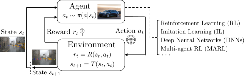
Figure 1. Agent-environment interaction in MDPs.

States $S$. $S$ is a set of states, and it’s also called the state space. It can be discrete or continuous. The state $s_{t}\in S$ describes the observations of the decision-making agent at timestep $t$.

Actions $A$. $A$ is a set of actions that an agent can take, also called the action space, which can be discrete or continuous.

Transitions $T$. $T$ is the state transition function $s_{t+1}=T(s_{t},a_{t})$. The state of the MDP is $s_{t}$ at timestep $t$, and the agent takes action $a_{t}$. The MDP will step into the next state $s_{t+1}$ according to $T$.

Rewards $R$. $R$ defines the immediate reward, which is also known as the “reinforcement.” At state $s_{t}$, the agent receives immediate reward $r_{t}=R(s_{t},a_{t})$ by taking action $a_{t}$.

Policy $\pi$. $\pi$ is the agent’s policy. $\pi(a|s_{t})$ is the probability distribution over possible actions. It estimates the cumulative rewards of taking action $a_{t}$ at state $s_{t}$. A deterministic agent will take the action that maximizes the estimated rewards according to its policy, i.e., the action with the highest probability given by $\pi(a|s_{t})$. Meanwhile, a stochastic agent will take an action according to the actions’ probability distribution over all actions given by $\pi(a|s_{t})$.

Markov property. We present the formal definition of Markov property in Definition 2.1. Markov property forms the basis of an important and unique optimization opportunity taken by MDPFuzz, as discussed in Sec. 5.2. The Markov property shows that the probability ($Pr$) of moving to the next state $s_{t+1}$ in an MDP depends solely on the present state $s_{t}$ and not on the previous states.

Definition 0 (Markov property).

The sequence of the states in MDP is a Markov chain, which has the following Markov property:

$$Pr(S_{t+1}=s_{t+1}|S_{t}=s_{t},\cdots,S_{0}=s_{0})=Pr(S_{t+1}=s_{t+1}|S_{t}=s_{t})$$

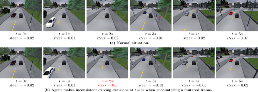
Figure 2. Inconsistencies focused by prior DNN testing do not always result in severe states in models solving MDPs.

Models Solving MDPs. To date, neural models are often used to form the agent policy $\pi$ in Fig. 1. They can thus solve sequential decision-making problems by modeling them as MDPs and obtaining the (nearly-)optimal policies. We now review four cutting-edge models, whose performance is close to or even better than humans.

Deep Neural Network (DNN). The supervised DNNs train an agent model to predict the best action $a_{t}$ at the present state $s_{t}$. It assumes that the present action $a_{t}$ is solely determined by the current state $s_{t}$, and states before $s_{t}$ have no influence. With enough manually labeled data, DNNs can model an agent policy even close to the optimal policy $\pi^{*}$. This technique has been used in autonomous driving systems developed by NVIDIA (Bojarski et al., 2016; Bojarski et al., 2017) and DNN-based variant of ACAS Xu (Julian et al., 2019) with impressive results.

Reinforcement Learning (RL). Supervised DNNs often require a significant amount of labeled data. Data labeling needs considerable human effort, which is unrealistic in many real-world situations. RL does not require labeled data. Instead, it uses reward functions in MDPs to guide the agent model in estimating the cumulative reward. A3C (Mnih et al., 2016), DDPG (Lillicrap et al., 2015), DQN (Mnih et al., 2013), PPO (Schulman et al., 2017), TQC (Kuznetsov et al., 2020), and other RL algorithms have emerged with impressive performance. These algorithms have been deployed in complex scenarios like Go (Silver et al., 2016), video games (Berner et al., 2019), and robot control (Kober et al., 2013), and their performance has been superior to that of humans.

Imitation Learning (IL) (Ho and Ermon, 2016). RL does not require a substantial amount of labeled data. However, defining reward functions might be tricky in some cases. IL comes in handy when it is easier for an expert to demonstrate the desired behavior than designing an explicit reward function. The MDP is the main component of IL, and the reward function $R$ is unknown to the agent. The IL agent can either learn the expert’s policy or estimate the reward function by monitoring the expert’s trajectories, which are sequences of states and actions $\tau=(s_{0},a_{0},s_{1},a_{1},\cdots)$. Waymo uses IL to learn an urban driving policy from human drivers (Bansal et al., 2018).

Multi-agent Reinforcement Learning (MARL) (Busoniu et al., 2008). MARL provides solutions for scenarios with multiple agents. In most cases, both the state and the reward received by each agent are influenced by the joint actions of all agents. Agents can cooperate to solve a problem, with the overall goal being to maximize the average cumulative rewards of all agents. The global cooperative optimum is a Nash equilibrium (Osborne and Rubinstein, 1994). The agents can also compete with one another, resulting in a zero-sum Markov game. MARL has been used to train agents in video games (Vinyals et al., 2019) and traffic control (Wiering, 2000; Qiu et al., 2019).

3. Related Work

Existing works have laid a solid foundation in testing DNNs (Zhang et al., 2020). We review these works holistically from three aspects to present a self-contained paper. We also particularly discuss existing works testing RL to motivate the design of MDPFuzz.

Target DNNs. Recurrent neural networks (RNNs) and feedforward neural networks (FNNs) are two representative types of DNNs. Given the wide adoption of FNNs in computer vision (CV), most existing works test FNNs have examined the accuracy of FNN-based image classifiers and their applications, such as autonomous driving systems (Pei et al., 2017; Zhang et al., 2018; Tian et al., 2018; Dwarakanath et al., 2018; Nakajima and Chen, 2019; Wang and Su, 2020; Yuan et al., 2021c, b, a). Natural language processing (NLP) models have also been tested (He et al., 2020; Sun et al., 2020; Ma et al., 2020; Ma and Wang, 2022). We also notice recent works on testing RNNs and RL models (Du et al., 2018, 2019; Guo et al., 2019; Huang et al., 2019; Uesato et al., 2018). DeepStellar (Du et al., 2019), a SOTA RNN testing work, models the target RNN’s internal state transition using Finite State Transducer (Gill et al., 1962) as a testing guide. DeepStellar requires a bounded RNN state space with reasonable size. This assumption may not hold for models solving MDPs, because the state space can often be unlimited, especially in real-world blackbox scenarios such as autonomous driving and robot control. Moreover, the transition functions $T$ in complex real-world MDP environments are difficult, if possible, to obtain. In contrast, MDPFuzz tests FNNs, RL, IL, and MARL models for solving MDPs using a unified approach.

Testing Oracle and Testing Criteria. Constructing proper oracles has long been difficult for testing DNNs (Zhang et al., 2020). Metamorphic or differential testing has been used extensively to overcome the difficulty of explicitly establishing testing oracles (Segura et al., 2016; Pei et al., 2017; Wang and Su, 2020; Chen et al., 2021). Consequently, DNNs are considered incorrect if they produce inconsistent results. However, Sec. 4 shows that “inconsistency” does not always lead to model anomalies. For instance, an autonomous driving model can easily recover from steering driftings. Regarding testing criteria selection, whitebox DNN testing relies on a wide range of coverage criteria (Pei et al., 2017; Ma et al., [n.d.]; Odena and Goodfellow, 2018; Sun et al., 2018). In contrast, blackbox testing may use evolutionary algorithms or other heuristics to determine test input quality (Xie et al., 2019b). Sec. 4 introduces MDPFuzz’s statistics-based methods for evaluating and prioritizing test inputs.

Input Mutation. Previous works testing CV models use pixel-level mutations (Pei et al., 2017), weather filters (Zhang et al., 2018), and affine transformations (Tian et al., 2018) for semantics-preserving changes on images. For natural language text, existing works often use pre-defined templates to generate linguistically coherent text (Galhotra et al., 2017; Udeshi et al., 2018; Ma et al., 2020; He et al., 2020). DNN models typically process each input separately. Models solving MDPs, however, constantly respond to a series of states, e.g., an autonomous driving model makes decisions about each driving scene frame captured by its camera. Changing arbitrary frames may destroy inter-state coherence; see MDPFuzz’s solution in Sec. 4.

Existing RL Testing. There exist several works that test RL (Uesato et al., 2018; Lee et al., 2020; Julian et al., 2020; Ernst et al., 2019; Koren et al., 2018; Yamagata et al., 2020). (Uesato et al., 2018) assumes that crash patterns in weaker RL models are similar to those in more robust RL models. During the training phase of RL models, crash-triggering sequences are collected to train a classifier to predict whether a (mutated) initial state would cause abnormal future states. This method relies heavily on historical training data, which also limits the method’s ability to discover new and diverse crash-triggering state sequences. (Lee et al., 2020; Julian et al., 2020; Ernst et al., 2019; Koren et al., 2018; Yamagata et al., 2020) adopt similar approaches to (Uesato et al., 2018) to find the crash-triggering path, but designing the scenario-specific algorithms is hard. Moreover, the training process needs a large amount of data simulation and its performance highly depends on the data sampling method. These works studied a specific model/scenario, and they do not aim to deliver a unified framework to test models solving MDPs. They train models to predict a path reaching an unsafe state instead of detecting numerous crashes efficiently. It is hard to adapt these methods to uncover numerous crash-triggering sequences in MDP scenarios, considering the high training/simulation cost. Besides, while MDPFuzz  leverages the Markov property, a unique property in MDP, to largely optimize the fuzzing efficiency (see Sec. 5.2), all prior works do not consider the Markov property.

4. Testing DNN Models Solving MDPs

This section describes the challenges that previous DNN testing works face when testing models solving MDPs. Accordingly, we introduce several design considerations of MDPFuzz.

Inconsistencies vs. Crashes. Most DNN testing works form testing oracles by checking prediction consistency, as reviewed in Sec. 3. However, such a testing oracle is overly strict when it comes to testing models solving MDPs. Consider Fig. 2, which depicts the behavior of the SOTA RL model (Toromanoff et al., 2020) that won Camera Only track of the CARLA challenge (car, [n.d.]a). We establish an autonomous driving scenario where the RL model decides the steer angles and speed per frame. Fig. 2a shows the RL model’s reaction to six frames. Then, we create an “inconsistent” driving behavior, at $t=2s$, by compelling the RL model to change its decision from virtually straight (0.02) to turning right (0.5). Existing works (Zhang et al., 2018; Tian et al., 2018) would consider such “inconsistent” driving behavior erroneous. However, as seen in Fig. 2b, the RL-controlled vehicle quickly returns to its normal state in the following frames, with steer approaching zero.

A well-trained model for solving MDPs (e.g., a robot controller) can frequently meet and recover from short-term inconsistencies. Inconsistent predictions do not always lead to abnormal or dangerous states. We thus present the following argument:

Table 1. Crash feasibility when the RL model yields multiple inconsistent decisions.

Inconsistent decision ratio	1%	5%	10%	25%	50%
Crash feasibility	0%	1.5%	2.3%	6.0%	11.5%

Example. Table 1 reports the relations between the ratio of inconsistent RL-model decisions in one autonomous driving run and the average feasibility of collisions (i.e., “Crash feasibility”). We run the autonomous driving model for 1,000 runs with randomly selected initial states. Each run stops at $t=10s$, thus generating 100 frames (10 fps). We randomly select several frames and change the RL-controlled vehicle in those frames by compelling their steering to either left most or right most (which rarely occur in normal driving). We find that when the RL-controlled vehicle in a single frame is mutated, equivalent to the 1% inconsistent decision ratio of Table 1, it cannot result in a collision across all 1,000 runs, and the vehicle recovers quickly from inconsistent decisions. The crash feasibility increases slightly when many decisions are changed into an inconsistent stage in a run. Even if half of the steering decisions are changed, only 11.5% of these runs can cause vehicle collisions. Mutating 50% of decisions induce apparently unrealistic driving behaviors. Comparatively, MDPFuzz  uncovers 164 collisions by only mutating the initial state without breaking the naturalness (see Sec. 6) of the entire MDP procedure, as shown in Sec. 7.

To ease reading, this paper refers to abnormal and dangerous states as “crashes.” We regard crashes incurred from a valid and solvable initial state as bugs of a model $\pi$ solving MDP. Formally, we have the following definition:

Definition 0 (Crash-triggering state sequences).

Given model $\pi$ and a valid and solvable initial state $S_{0}$, we observe a state sequence: $\{S_{t}\}_{t\in[M-1]}$, whose actions are made by $\pi$. $S_{0}$ is regarded as crash-triggering if there exists a crash state $S_{t}(t>0)$.

We require that $S_{0}$ is solvable for an optimal model $\pi^{*}$, meaning that every state in the optimal state sequence $\{S_{t}^{*}\}_{t\in[M-1]}$ is not a crash state. Therefore, Def. 4.1 implies that $\pi$ is buggy, whose bug-triggering input is $S_{0}$. We, clarify that “crash” (i.e., testing oracle) is defined case by case; see Testing Oracles in Sec. 6.

Mutating Initial States vs. Mutating Intermediate States. Mutating arbitrary frames in an MDP can enlarge the testing surface of the target model and potentially reveal more defects. Mutating an intermediate frame, however, could break the coherence of an MDP state sequence. In Fig. 2, our tentative study shows that by mutating the surrounding environment in the driving scene at frame $t$, it is possible to influence the RL-controlled vehicle’s decision. However, given such mutations introduce broken coherence when considering frames around $t$, defects found by mutating frame $t$ may not imply real-world anomaly behaviors of autonomous driving vehicles. We thus decide to only mutate the initial state (e.g., re-arrange the environment at timestep $0$), allowing to preserve the coherence of the entire MDP state sequence. For each MDP scenario, we validate mutated initial states in a deliberate way to ensure they are realistic and solvable for an optimal model $\pi^{*}$; see MDP Initial State Sampling, Mutation, and Validation in Sec. 6.

Design Overview. MDPFuzz is designed to evaluate blackbox models (not merely RL) solving MDPs. MDPFuzz requires no training phase information (in contrast to (Uesato et al., 2018)). Our testing oracle checks abnormal and dangerous states instead of models’ inconsistent behaviors (see Sec. 6 for our oracles). Moreover, we only mutate the initial state rather than arbitrary states to generate more realistic scenarios. These new designs add to the complexity and cost of testing models solving MDPs. Worse, earlier objective-oriented generation methodologies (Pei et al., 2017), which rely on loss functions to directly synthesize corner inputs, are no longer feasible because MDP transition functions $T$ are often unavailable and not differentiable.

MDPFuzz offers a comprehensive and unified solution to all of the issues above. It incorporates several optimizations to maintain and prioritize initial states with greater potential to cover new model behaviors. Our evaluation reveals promising findings when testing real-world models under various MDP scenarios.

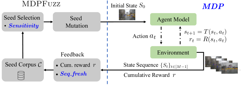
Figure 3. Workflow. The “Agent Model” is the testing target.

5. Design

Assumptions. Fig. 3 illustrates the workflow of MDPFuzz. In blackbox settings, the internal of the agent model (our testing target) is not revealed to MDPFuzz. Similarly, the MDP transition function $T$ and reward function $R$ in the environment are unavailable. However, MDPFuzz can collect the state sequence $\{S_{t}\}_{t\in[M-1]}$ went through by the target model and obtain the cumulative reward $r$ from the environment. For instance, when testing autonomous driving models, MDPFuzz can collect a series of frames that the autonomous driving model captures from the environment and obtain the cumulative reward $r$ corresponding to this series. We clarify that this assumption is realistic, even for (commercial) blackbox models. As noted above, MDPFuzz has no access to the blackbox model internals. However, in a typical MDP environment, the states and agent actions are observable and the rewards are calculated based on the observed states. No additional information is needed. MDPFuzz only mutates the initial state $S_{0}$ of an MDP, under the constraint that it is still realistic and solvable after mutation. See Sec. 6 on how mutated initial states are validated in this study.

Alg. 1 formulates the fuzz testing procedure, including key components mentioned in Fig. 3. Fuzzing is the main entrance of Alg. 1, which returns the set of error-triggering initial states $\mathcal{R}$, forcing the target model to enter severe states (e.g., collisions in autonomous driving). As we have discussed in Definition 4.1, we refer to such severe states as “crashes” in this paper. We summarize functions corresponding to the key components of Fig. 3 as follows:

• MDP starts from the initial state $S_{0}$ and observes the interaction between the target agent model and the environment for $M$ timesteps (line 2). It returns the sequence of covered states and the cumulative reward (line 3). The length $M$ of the state sequence is a hyper-parameter.

• Sensitivity estimates the sensitivity of the target model against MDPFuzz’s mutations on the initial states (see Sec. 5.1). A larger sensitivity indicates that the model becomes less robust (a good indicator for testing) w.r.t. the mutated initial states. This is comparable to estimating seed energy in software fuzzing (Böhme et al., 2017; Chen et al., 2017).

• Seq_fresh estimates the state sequence “freshness” (see Sec. 5.2). Overall, it checks whether a sequence of covered states has new patterns that do not exist in previously-found sequences. This is comparable to taking code coverage as feedback in software fuzzing (Zalewski, 2021; Klees et al., 2018). Note that MDPFuzz can observe state sequence in blackbox settings.

Algorithm 1 MDPFuzz workflow

1:function MDP($S_{0}$)

2:$\triangleright$   ObserveFromEnv: run agent-env interaction for $M$ steps

3:    $r$, $\{S_{t}\}_{t\in[M-1]}$ $\leftarrow\textsc{ObserveFromEnv}(S_{0})$

4:    return $r$, $\{S_{t}\}_{t\in[M-1]}$

5:function Fuzzing( )

6:$\triangleright$   $\tau$: state sequence freshness threshold

7:    $\mathcal{C}\leftarrow\textsc{Sampling}(N)$ $\triangleright$Sample seed corpus with $N$ initial states

8:    $Params^{s},Params^{c}\leftarrow\textsc{Init()}$ $\triangleright$Initialize key parameters

9:    for $S_{0}^{i}\in\mathcal{C}$ do

10:        $E_{i}\leftarrow{\color[rgb]{0,0,1}\textsc{{{Sensitivity}}}}(S_{0}^{i})$

11:        $r_{i},\{S_{t}^{i}\}_{t\in[M-1]}\leftarrow{\color[rgb]{0,0,1}\textsc{{{MDP}}}}(S_{0}^{i})$

12:        $p_{i}\leftarrow{\color[rgb]{0,0,1}\textsc{{{Seq_fresh}}}}(\{S_{t}^{i}\}_{t\in[M-1]},Params^{s},Params^{c},\tau)$     

13:    while passed time $<12$ hours do

14:        Select $S_{0}^{k}$ from $\mathcal{C}$ with probability $E_{k}/\sum_{i=1}^{N}E_{i}$

15:        $S_{0}^{\Delta,k}\leftarrow\textsc{Mutate_Validate}(S_{0}^{k})$

16:        $r_{k}^{\Delta},\{S_{i}^{\Delta,k}\}_{i\in[M-1]}\leftarrow{\color[rgb]{0,0,1}\textsc{{{MDP}}}}(S_{0}^{\Delta,k})$

17:        $p_{k}^{\Delta}\leftarrow{\color[rgb]{0,0,1}\textsc{{{Seq_fresh}}}}(\{S_{i}^{\Delta,k}\}_{i\in[M-1]},Params^{s},Params^{c},\tau)$

18:        if $Crash(\{S_{i}^{\Delta,k}\}_{i\in[M-1]})$ then $\triangleright$Testing oracles. See Sec. 6 for details.

19:           Add $S_{0}^{\Delta,k}$ to $\mathcal{R}$

20:        else if $r_{k}^{\Delta}<r_{k}$ or $p_{k}^{\Delta}<\tau$ then $\triangleright$Feedback. See Sec. 5.3 for details.

21:           Add $S_{0}^{\Delta,k}$ to $\mathcal{C}$

22:           $E_{k}^{\Delta}\leftarrow{\color[rgb]{0,0,1}\textsc{{{Sensitivity}}}}(S_{0}^{\Delta,k})$

23:           Maintain $r_{k}^{\Delta},E_{k}^{\Delta},p_{k}^{\Delta}$ for $S_{0}^{\Delta,k}$             

24:    return $\mathcal{R}$

Initialization. Lines 5–10 in Alg. 1 initializes the fuzzing campaign of MDPFuzz. Line 5 randomly samples $N$ initial states in the legitimate state space of MDP to form the seed corpus $\mathcal{C}$ (see Sec. 6 for details). Then, the key parameters, $Params^{s}$ and $Params^{c}$, are initialized at line 6. Holistically speaking, these parameters maintain the up-to-date density distribution over previously-covered sequences, and it will be used by Seq_fresh to decide the freshness of a new sequence, as will be introduced in Sec. 5.2. We iterate each seed $S_{0}^{i}$ in corpus $\mathcal{C}$ and estimate its energy $E_{i}$ at line 8. Then, we feed $S_{0}^{i}$ to the target model, receive the state sequence $\{S_{t}^{i}\}_{t\in[M-1]}$ and its cumulative reward $r_{i}$ by running MDP (line 9), and compute the sequence freshness $p_{i}$ using Seq_fresh (line 10).

States Validation. We randomly mutate a selected seed (line 13). Seed mutation is bounded in the legitimate state space of MDP to guarantee that such initial states exist and solvable in real-world scenarios. We also use the validation module shipped by some MDP environments to validate the mutated states. In short, we clarify that all the mutated initial states are valid and solvable, and all the crashes we found are avoidable if the models can take the optimal actions (though currently the tested model failed to take the optimal actions and is thus buggy). See implementation details of Mutate_Validate in MDP Initial State Sampling, Mutation, and Validation of Sec. 6.

Fuzzing. As a common setup, MDPFuzz launches each fuzzing campaign for 12 hours (Klees et al., 2018). Each time (line 12) we select a seed $S_{0}^{k}$ from the corpus $\mathcal{C}$ with probability $\frac{E_{k}}{\sum_{i=0}^{N-1}E_{i}}$, where $E_{i}$ denotes the energy (estimated by Sensitivity) of the $i^{th}$ seed. Similar to software fuzzing which spends more time on seeds of higher energy (Zalewski, 2021; Böhme et al., 2017), MDPFuzz  prioritizes seeds with higher energy. We feed $S_{0}^{\Delta,k}$ to MDP, and collect the cumulative reward $r_{k}^{\Delta}$ and the state sequence $\{S_{i}^{\Delta,k}\}_{i\in[M-1]}$ (line 14). If the new initial state can cause a crash according to our oracle, we add it to the crash-triggering set $\mathcal{R}$ (lines 16–17).

Line 15 measures the freshness of the covered state sequence, quantifying how much the new sequence is distinct with previously-covered sequences. Then, we check whether the new cumulative reward $r_{k}^{\Delta}$ is smaller than the reward collected when using $S_{0}^{k}$, or whether the freshness is above a threshold (line 18). If so, we keep $S_{0}^{\Delta,k}$ in the seed corpus (line 19) and also maintain its associated reward, energy, and sequence freshness for future usage.

5.1. Robustness & Sensitivity

Sensitivity estimates a seed’s potential to provoke diverse behaviors of the target model. Notably, the resilience of the model solving MDPs is commonly defined in terms of their sensitivity to state permutations. Many previous works have launched adversarial attacks by adding small permutations to the observed states of RL models (Xiao et al., 2019; Pattanaik et al., 2017; Behzadan and Munir, 2017; Kos and Song, 2017).

Algorithm 2 Sensitivity estimation.

1:function Sensitivity($S_{0}$)

2:    $S_{0}^{\Delta}\leftarrow S_{0}+\Delta S$ $\triangleright$$\Delta S$ is a small random permutation

3:    $r,\{S_{t}\}_{t\in[M-1]}\leftarrow{\color[rgb]{0,0,1}\textsc{{{MDP}}}}(S_{0})$,   $r_{\Delta},\{S_{t}^{\Delta}\}_{t\in[M-1]}\leftarrow{\color[rgb]{0,0,1}\textsc{{{MDP}}}}(S_{0}^{\Delta})$

4:    return $\frac{|r-r_{\Delta}|}{||\Delta S||_{2}}$

Inspired by these works, the potential of a seed, i.e., an initial state $S_{0}$, is estimated by the sensitivity of the target model w.r.t. randomness in $S_{0}$. As shown in Alg. 2, Sensitivity adds small random permutations $\Delta S$ to an initial state $S_{0}$ and then collects the cumulative reward $r_{\Delta}$ from MDP. The local sensitivity of the model at $S_{0}$ can thus be estimated by $\frac{|r-r_{\Delta}|}{||\Delta S||_{2}}$, where $r$ is the cumulative reward without permutation. Interested readers may refer to an illustrative example of Alg. 2’s intuition at (sna, [n.d.]).

5.2. State Sequence Freshness & DynEM

Seq_fresh in Alg. 1 guides MDPFuzz to promptly identify “fresh” state sequences. Software fuzzing keeps mutated seeds if new coverage patterns are exposed (Zalewski, 2021). Similarly, MDPFuzz keeps a mutated initial state if its induced state sequence is distinct from previously covered sequences (line 18 in Alg. 1). Neuron coverage (Pei et al., 2017), a common criterion in DNN testing, is not proper here; see Sec. 8.

Motivation. A naive way to measure the freshness between a new state sequence and previously covered sequences is to calculate the minimum distance between them iteratively. Table 2 compares a naive distance-based method with Seq_fresh. We use the setting of RL for CARLA assessed in Sec. 4, where the state sequence length is 100, and each agent state’s dimension is 17. Given a new state sequence, the distance-based method iterates all historical sequences (“corpus size” in Table 2) for comparison. Calculating the distance between a new sequence and all existing sequences in the corpus takes roughly a minute when the corpus size is 1,000, which is too costly considering that there are thousands of mutations in a 12-hour run, as will be reported in Sec. 7.1.

Estimating Freshness with Constant Cost. MDPFuzz proposes to first estimate a probability density function (pdf) with existing state sequences. Then, comparing a new state sequence with existing sequences is recast to calculating the density of the new sequence by the pdf. A new sequence emitting low density indicates that it’s not covered by existing sequences. That is, low density indicates high freshness.

Enabled by DynEM (introduced soon), MDPFuzz can measure the freshness of a new sequence with the pdf of all existing sequences in one run. Further, benefiting from the Markov property introduced in Definition 2.1, we only need to estimate two separate pdfs with much smaller input spaces than the entire sequence. The cost of each comparison becomes thus constant and modest. In reality, Seq_fresh only takes 0.25 seconds for tasks benchmarked in Table 2 and does not scale with corpus size. Recent software fuzzing (Manès et al., 2020) uses PCA-based approaches (Wold et al., 1987) which are not applicable here; see discussion in Sec. 8.

Seq_fresh. Overall, Alg. 3 estimates $Pr(S_{t})$ and $Pr(S_{t+1},S_{t})$, as shown in the following joint pdf of a state sequence:

(1) $$\begin{split}Pr(\{S_{t}\}_{t\in[M]})=Pr(S_{M},\cdots,S_{0})=Pr(S_{0})\prod_{t=0}^{M-1}Pr(S_{t+1}|S_{t})=Pr(S_{0})\prod_{t=0}^{M-1}\frac{Pr(S_{t+1},S_{t})}{Pr(S_{t})}\end{split}$$

Aligned with convention (Belghazi et al., 2018; Fei-Fei et al., 2006; Hjelm et al., 2018) in machine learning, we use Gaussian mixture models (GMMs) (McLachlan and Basford, 1988) to estimate the pdfs, given that GMMs can estimate any smooth density distribution (Goodfellow et al., 2016). Then, Eq. 1 is re-written in the following form:

(2) $$\begin{split}Pr&(\{S_{t}\}_{t\in[M]})=GMM^{s}(S_{0})\prod_{t=0}^{M-1}\frac{GMM^{c}(S_{t+1}||S_{t})}{GMM^{s}(S_{t})}\\ &=(\sum_{k=0}^{\mathcal{K}-1}\phi_{k}^{s}\mathcal{N}(S_{0}\,|\,\mu_{k}^{s},\Sigma_{k}^{s}))\prod_{t=0}^{M-1}\frac{\sum_{k=0}^{\mathcal{K}-1}\phi_{k}^{c}\mathcal{N}(S_{t+1}||S_{t}\,|\,\mu_{k}^{c},\Sigma_{k}^{c})}{\sum_{k=0}^{\mathcal{K}-1}\phi_{k}^{s}\mathcal{N}(S_{t}\,|\,\mu_{k}^{s},\Sigma_{k}^{s})}\end{split}$$

, where $\mathcal{N}$ is the pdf of Gaussian distribution, $\{\phi_{k}^{s},\mu_{k}^{s},\Sigma_{k}^{s}\}_{k\in[\mathcal{K}-1]}$ are parameters of the GMM estimating single state pdf $Pr(S_{t})$, $s$ in the superscript denotes “single,” $\{\phi_{k}^{c},\mu_{k}^{c},\Sigma_{k}^{c}\}_{k\in[\mathcal{K}-1]}$ are parameters of the GMM estimating concatenated states pdf $Pr(S_{t+1},S_{t})$, and $c$ denotes “concatenated.” Eq. 2 forms the basis of Seq_fresh as in Alg. 3. Thus, to calculate Seq_fresh, we only need the parameters of the two GMMs: $\{\phi_{k}^{s},\mu_{k}^{s},\Sigma_{k}^{s},\phi_{k}^{c},\mu_{k}^{c},\Sigma_{k}^{c}\}_{k\in[\mathcal{K}-1]}$ in Eq. 2. We develop DynEM to estimate and update these parameters efficiently based on the state sequences MDPFuzz has already covered.

Table 2. Cost of distance-based method and Seq_fresh.

Corpus size	100	500	1,000	3,000
Processing time (sec) of distance-based method	5.31	26.10	54.19	156.87
Processing time (sec) of Seq_fresh	0.25

Algorithm 3 State sequence freshness.

1:function Seq_fresh($\{S_{t}\}_{t\in[M-1]}$, $Params^{s}$, $Params^{c}$, $\tau$)

2:    for $t\in[M-2]$ do

3:        $p(S_{t})\leftarrow\textsc{GMM}(S_{t},Params^{s})$

4:        $p(S_{t},S_{t+1})\leftarrow\textsc{GMM}(S_{t}||S_{t+1},Params^{c})$     

5:    $p\leftarrow p(S_{0})\times\prod_{t=0}^{M-2}\frac{p(S_{t},S_{t+1})}{p(S_{t})}$

6:    if $p<\tau$ then

7:        $Params^{s},Params^{c}\leftarrow\textsc{DynEM}(\{S_{t}\}_{t\in[M-1]},Params^{s},Params^{c})$     

8:    return $p$

DynEM. Unlike expectation-maximization (EM) (Dempster et al., 1977), which re-computes the estimation whenever the seed corpus is updated, DynEM in Alg. 3 estimates the GMM parameters in an online and incremental manner. Thus, DynEM greatly reduces the computation cost of EM while achieving the asymptotic equivalence to the EM algorithm (Cappé and Moulines, 2009). We adopt the ideas proposed in the online EM algorithm (Cappé and Moulines, 2009) and extend it to estimate the parameters of GMMs. Instead of calculating the parameters of GMMs directly, DynEM updates the complete and sufficient (C-S) statistics (Casella and Berger, 2021) every time MDPFuzz finds a new state sequence. In short, to estimate the parameters of the pdf, we only need its corresponding C-S statistics, and the parameters of Eq. 2 can be directly derived from the C-S statistics parameters of DynEM, which contain all the information we need and correspond to $Params^{s}$ and $Params^{c}$. Also, when MDPFuzz finds a new state sequence, $Params^{s}$ and $Params^{c}$ are updated in DynEM, and consequently, updating the parameters of Eq. 2. This way, Seq_fresh can maintain the up-to-date pdf of all covered sequences. Details of GMM and DynEM are omitted; see the full algorithm, the explanation of C-S statistics, and clarification on all the employed statistics mechanisms at our artifact (sna, [n.d.]).

$Params^{s}$ and $Params^{c}$ in Alg. 3 are randomly initialized (line 6 in Alg. 1). When a new state sequence $\{S_{t}\}_{t\in[M]}$ is found by MDPFuzz, its sequence density $p$ is calculated following Eq. 2 (lines 3–5 in Alg. 3). If its density $p$ is smaller than the threshold $\tau$, meaning that we find a fresh sequence, we use DynEM to update the key parameters, thereby updating our maintained pdf of existing state sequences (lines 6–7 in Alg. 3).

5.3. Feedback from Freshness & Reward

The fuzzing feedback is derived from the state sequence freshness and the cumulative reward. This corresponds to line 18 in Alg. 1.

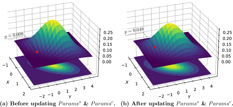
Figure 4. Illustration of Alg. 3.

Freshness. Fig. 4 illustrates the use of freshness to guide fuzzing. When MDPFuzz finds a new state sequence (the red dot in Fig. 4), we compute the sequence density ($p=0.008$; line 15 in Alg. 1), which is lower than the threshold $\tau=0.01$. The mutated initial state is then added to the corpus (line 19 in Alg. 1), and DynEM also updates $Params^{s}$ and $Params^{c}$. Following this update (Fig. 4b), the newly-discovered sequence density increases to $p=0.048$. In the future, similar sequences will have densities of approximately $p=0.048$ (greater than $\tau$), and they will not be added to the corpus unless they can reduce the cumulative reward (see below). When DynEM is constantly fed with new sequences, the estimated sequence density distribution becomes increasingly wider, e.g., comparing the covered area by the distribution in Fig. 4b with that in Fig. 4a. This reflects that MDPFuzz keeps finding new state sequences that can occur in MDP. The efficiency of Seq_fresh is evaluated in Sec. 7.2.

Cumulative Reward. MDPFuzz is also guided by cumulative rewards. Typically, when a model is trained for solving MDPs, reward functions are needed to maximize the state sequences’ cumulative rewards. For example, autonomous driving models are penalized, with small (negative) rewards, if they collide, run red lights, violate the speed limit, or commit other infractions. Models are rewarded positively if they follow the scheduled routine and move towards the destination. We use the cumulative reward to quantify the target model’s behavior. A low cumulative reward suggests a high risk of catastrophic failures. MDPFuzz prioritizes mutated initial states that can reduce the cumulative rewards. Particularly, let an initial state $S_{0}^{\Delta,k}$ be mutated from $S_{0}^{k}$, we retain $S_{0}^{\Delta,k}$ in the seed corpus if the new state sequence starting from $S_{0}^{\Delta,k}$ induces a lower cumulative reward than that of $S_{0}^{k}$ (line 18 in Alg. 1).

6. Implementation & Evaluation Setup

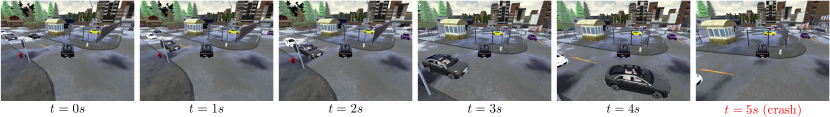
Figure 5. Crash triggering sequence found by MDPFuzz. (Please refer to (sna, [n.d.]) for more results.)

MDPFuzz is written in Python with approximately 1K LOC. It can be integrated to test different models solving MDPs. We use Scipy (ver. 1.6) and NumPy (ver. 1.19) for GMM and DynEM calculation. We run all tested models on PyTorch (ver. 1.8.0). Given an initial state $S_{0}$, MDP in Alg. 1 measures $M$ sequential states, and we set adequately large $M$ for different models. In short, if the agent’s states change rapidly, we may use a smaller $M$, and vice versa. Table 3 reports $M$ (“#Frames”) for each setting. Users can increase $M$ to stress particularly robust models. Each fuzzing campaign takes 12 hours, as a standard setting (Klees et al., 2018). Before that, we randomly sample for two hours to create the initial seed corpus (lines 5–10 in Alg. 1). We report that our sampled initial seeds produce almost no crashes for our tested models, e.g., throughout the 2 hours of seed sampling of CARLA RL, just one state sequence triggered a crash, and similar observations were made over other datasets. Experiments are launched on a machine with one AMD Ryzen CPU, 256GB RAM, and one Nvidia GeForce RTX 3090 GPU.

Target Models and Environments. CARLA (Dosovitskiy et al., 2017) is a popular autonomous driving simulator. MDPFuzz tests SOTA RL and IL models (Toromanoff et al., 2020; Chen et al., 2020) in CARLA. The RL model won the Camera Only track of the CARLA competition (car, [n.d.]a), and the IL model is currently ranked #1 in the CARLA leaderboard (car, [n.d.]b). They determine steering and acceleration using images collected by the vehicle’s camera as inputs. ACAS Xu (Marston and Baca, 2015) is a collision avoidance system for airplanes. In this work, we focus on the DNN-based variant of ACAS Xu (Julian et al., 2019), which has promising performance and much less memory requirement than the original ACAS Xu. It is also well-studied by existing DNN verification work (Wang et al., 2018). The DNN-based ACAS Xu uses 45 distinct neural networks to predict the best actions, such as clear of conflict, weak/strong left and right turns. Cooperative Navigation (Coop Navi) (Lowe et al., 2017) is an OpenAI-created environment for MARL. Coop Navi requires agents to cooperate to reach a set of landmarks without colliding. We use OpenAI’s release code to train the model to the performance stated in their article (Lowe et al., 2017). The MARL models use each agent’s position and target landmarks to decide their actions (e.g., moving direction and speed). Another RL model is for the OpenAI Gym BipedalWalker environment (Kuznetsov et al., 2020). In BipedalWalker, the agent attempts to walk through grasslands, steps, pits, and stumps. We use the publicly available TQC (Kuznetsov et al., 2020) model from the well-known stablebaseline3 repository (Raffin, 2020), which takes a 24-dimension state as input and predicts the speed for each leg based on body angle, leg angles, speed, and lidar data.

Testing Oracles (Crash Definition). For RL and IL models in CARLA, we examine whether the model-controlled vehicle collides with other vehicles or buildings. For DNN-based ACAS Xu, we check collisions of the DNN-controlled airplane with other airplanes. For Coop Navi, we check collisions between MARL-controlled agents. For BipedalWalker, we check whether the RL-controlled walking agent falls (i.e., its head touches the ground).

As expected, the crash or abnormal state is defined case by case, and orthogonal to MDPFuzz. Users can configure MDPFuzz with other undesired behaviors as long as such abnormal states can induce reasonably low rewards. In sum, we deem that the abnormal state definition is not restricted to certain scenarios, and we evaluate MDPFuzz on multiple models across multiple scenarios to alleviate potential concern that MDPFuzz won’t generalize.

MDP Initial State Sampling, Mutation, and Validation. As aforementioned, the initial states of MDPs (e.g., the positions of all participants) serve the test inputs. MDPFuzz samples (line 5 in Alg. 1) and mutates (line 13) MDP initial states. In brief, we emphasize that:

We add random noise to the initial states and the noise type depends on type of the original data, e.g., adding small Gaussian float numbers from $N(0,1)$ to vehicles’ initial positions, and adding small uniform integers from $U(0,4)$ to the ground type in BipedalWalker. We use a similar strategy to add small random permutations in Sensitivity.

Particularly, in CARLA, we change the initial positions and angles of all 100 vehicles, including the model-controlled vehicle. Note that CARLA validates and rejects abnormal initial states: all mutated initial states passed its validation. The model-controlled car’s initial speed is zero, and the environments guarantee other vehicles won’t cause crashes, such that the optimal actions (e.g., stop) can always avoid the crash. In DNN-based ACAS Xu, we mutate the initial positions and speeds of the model-controlled and the other planes. Moreover, we bound the maximal speed of all airplanes below 1,100 ft/sec, which is within the range of normal speed that a plane can reach in DNN-based ACAS Xu. We guarantee that there exist optimal actions to avoid the crash and solve the initial states, and we do not use an initial state that is not solvable. In Coop Navi, we mutate the initial positions of the three agents controlled by MARL. These initial positions prevent agents from colliding, and their initial speeds are 0. Our mutated initial states can pass Coop Navi’s initial state validation module, and we confirm there exist optimal solutions to avoid the crashes for our mutated initial states. In BipedalWalker, we modify the environment’s ground by mutating the sequence of the ground type the agent meets, e.g., in “flat, $\cdots$, stairs, flat, stump, $\cdots$”, the first 20 frames are “flat” to ensure that the agent does not fail initially. We then place a “flat” between two hurdles such that the agent can pass the obstacles when taking optimal actions.

7. Evaluation

Overview. We have reported the evaluation setup in Sec. 6. In evaluation, we mainly explore the following research questions. RQ1: Can MDPFuzz efficiently find crash-triggering state sequences from multiple SOTA models that solve MDPs in varied scenarios? RQ2: Can MDPFuzz be efficiently guided using the state sequence freshness (Seq_fresh), and can it cover more state sequences than using cumulative reward-based guidance alone? RQ3: What are the characteristics and implications of crash-triggering states? RQ4: Can we use MDPFuzz’s findings to enhance the models’ robustness? We answer each research question in one subsection below.

Table 3. Result overview

Model	MDP Scenario	#Frames	#Mutations	#Crashes
RL	CARLA autonomous driving	100	3,476.7 ($\pm$ 165.3)	161.7 ($\pm$ 10.4)
DNN	DNN-based ACAS Xu	100	161,542.7 ($\pm$ 1,226.2)	135.7 ($\pm$ 12.7)
	aircraft collision avoidance
IL	CARLA autonomous driving	200	3,166.7 ($\pm$ 25.0)	88.0 ($\pm$ 7.0)
MARL	Coop Navi game	100	531,200.3 ($\pm$ 1,983.5)	80.7 ($\pm$ 4.9)
RL	BipedalWalker game	300	6,602.0 ($\pm$ 149.5)	124.0 ($\pm$ 10.0)

Figure 6. Running time of MDPFuzz.

7.1. RQ1: Performance on Finding Crashes

Setup. We use the evaluation setup described in Sec. 6. That is, we launch MDPFuzz to fuzz each MDP model (listed in Table 3) and detect crashes. We collect all error-triggering inputs for analysis.

Results. Table 3 summarizes the findings of fuzzing each model. We report the average mutation and crash numbers and the corresponding standard deviation of three runs. Overall, MDPFuzz detects a significant number of crashes from all test cases. Within the 12-hour fuzzing, MDPFuzz generates more mutated initial states for the DNN-based ACAS Xu and Coop Navi cases. This is because the agents take less time to interact with the environments in these two cases; see the processing time evaluation below. Fig. 5 reports a crash found by MDPFuzz on the RL model used for the CARLA autonomous driving scenario. At timestep $t=0s$ (our mutated initial state), the speed of the agent vehicle (the black car in the middle of Fig. 5) is $0$, and it has no collisions with any other vehicles or buildings. During timesteps $t=1\sim 5s$, we observe that the RL model accelerates the vehicle without adjusting its steering. Hence, instead of turning left or moving in reverse, the vehicle hits the fence when $t=5s$. Overall, MDPFuzz can consistently reveal defects of models solving MDPs despite that they have different model paradigms or under distinct scenarios. We view this illustrates the strength and generalization of MDPFuzz. On the other hand, previous works have rarely focused on or systematically tested these models. Ignoring their potential defects will likely result in fatal incidents in real-world autonomous driving, airplane control, and robot control systems. We present the videos of the crashes found in other models at (sna, [n.d.]).

We report the time spent on each model in Fig. 6. In most cases, the target model’s computation and the interaction between the agent and the environment occupy most time. MDPFuzz only introduces a small overhead, considering that interaction in complex MDP environments is very time-consuming. Unlike other systems, the environments of DNN-based ACAS Xu and Coop Navi are simpler and do not consider physical effects. Therefore, these two systems can be accelerated, where one second in the real-world only requires approximately 6.36 ms and 23.97 ms in the DNN-based ACAS Xu (Simulate) and Coop Navi (Simulate), respectively. We accordingly set up these two simulation systems and re-run 12-hour fuzzing, whose results are also reported in Fig. 6. As expected, more computational resources are allocated to MDPFuzz. In sum, we deem that the cost of MDPFuzz is reasonable, especially when testing models solving complex MDPs. We also encourage users to configure their target environment in the “simulation” mode whenever possible to leave MDPFuzz more time for fuzzing.

7.2. RQ2: Efficiency & State Coverage

Setup. We use the same setting as that used in Sec. 7.1, and we compare the performance of MDPFuzz with and without the guidance of state sequence freshness computed by Seq_fresh. We run fuzz testing with these two versions of MDPFuzz on the models mentioned in Sec. 6 for 12 hours. As we mentioned in Sec. 5.2, the GMMs and DynEM are used to estimate the state sequence freshness. Thus, we can compare the covered areas of the two fuzzers by visualizing the distributions of their estimated GMMs.

Results. As shown in Fig. 7, we use the dashed lines to represent #crashes without the sequence freshness guidance. That is, MDPFuzz is only guided by the cumulative reward (line 18 of Alg. 1). We observe that with the same initial seed corpus when MDPFuzz is not guided by the sequence freshness, #crashes (dashed lines) is much smaller than when it is guided by both the cumulative rewards and sequence freshness (solid lines). We view this comparison as strong evidence to show the usefulness of sequence freshness. Note that Fig. 7 depicts the run with the median number of crashes across three separate runs, and as indicated in Table 3, the results of MDPFuzz are consistent, with a small standard deviation.

When testing DNN-based ACAS Xu, we observe that during the first four hours, the performance of the two setups is close because the environment of DNN-based ACAS Xu is simpler than other scenarios, and its model’s input dimension is small (only 5). However, after four hours, MDPFuzz can hardly find any new crashes, without the sequence freshness guidance. It terminates soon since it runs out of seeds without increasing any cumulative rewards. In contrast, with the sequence freshness guidance, MDPFuzz can proceed further and find 37 more crashes in the following eight hours. Given that the initial seed corpus for both settings is the same, we deem it efficient to use the state sequence freshness to guide MDPFuzz in testing the models of DNN-based ACAS Xu.

We use GMMs and DynEM to estimate the distributions of the sequences MDPFuzz has found, whose rationality has been demonstrated in Sec. 5.2. We visualize the GMMs estimated when testing the RL model for CARLA in Fig. 8, where Fig. 8a and Fig. 8b illustrate the estimated distributions for MDPFuzz without and with the state sequence freshness guidance, respectively. We project the $X$ and $Y$ axes to the same scale to compare the covered areas fairly. Comparing the space covered by these two distributions, we conclude that the guidance of state sequence freshness helps MDPFuzz cover a larger state sequence space. Thus, this guidance can boost the efficiency of MDPFuzz in progressively finding diverse state sequences. GMMs visualization results for other models are at (sna, [n.d.]).

Figure 7. #Crashes found w/ and w/o freshness guidance.

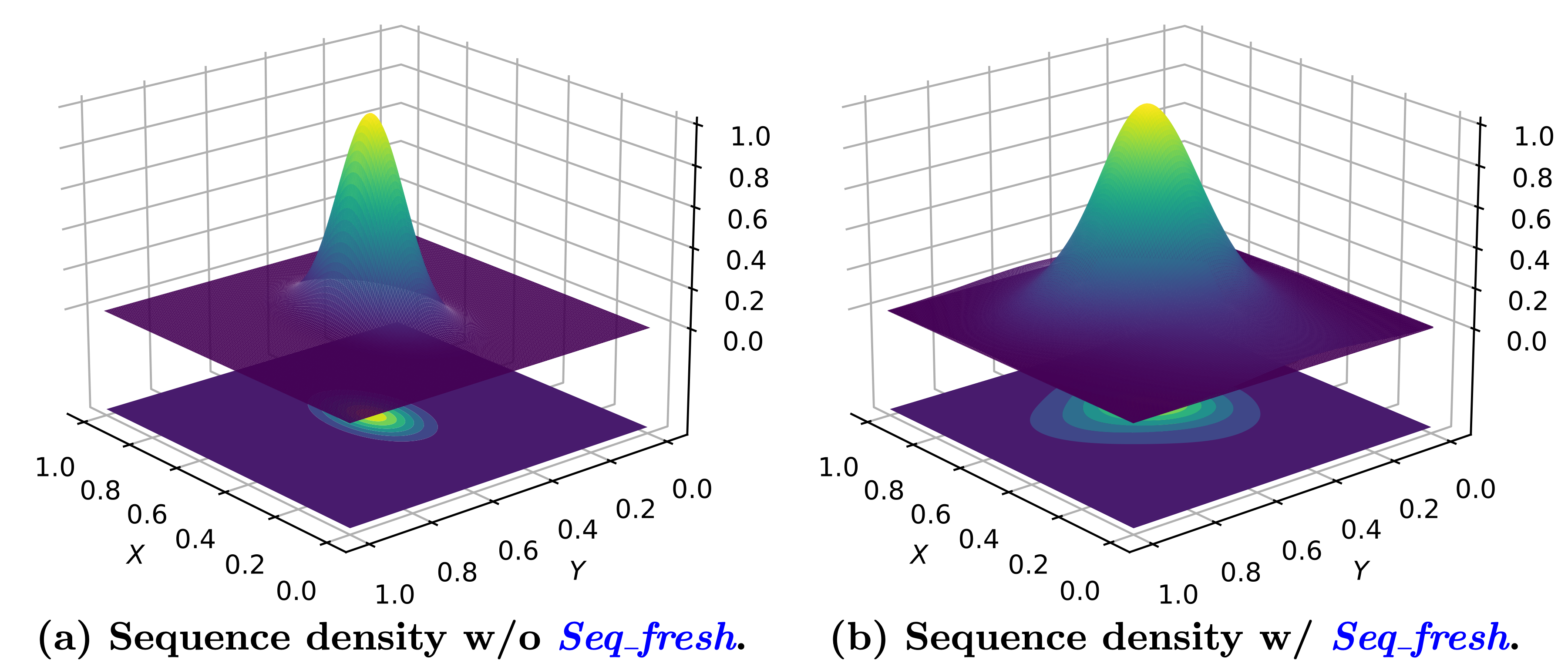
Figure 8. State coverage w/o and w/ freshness guidance.

7.3. RQ3: Root Cause Analysis

(a) RL for CARLA.

(b) DL of DNN-ACAS Xu.

(c) IL for CARLA.

(d) MARL for Coop Navi.

(e) RL for BipedalWalker.

Figure 9. Neuron activations projected by t-SNE.

Setup. Inspired by contemporary DNN testing criteria (Xie et al., 2019a; Pei et al., 2017; Ma et al., [n.d.]; Odena and Goodfellow, 2018), we characterize crash-triggering states by measuring their induced neuron activation patterns in all tested models. In this step, we take a common approach to use t-SNE (Van der Maaten and Hinton, 2008) to reduce dimensions and visualize the distributions of activated neurons.

Results. Fig. 9 visualizes and compares the states’ neuron activations of the target models. We plot the activation patterns of the states in sequences when their initial states are crash-triggering (red dots), normal (blue dots), and randomly-mutated (teal dots). The neuron activations are projected to two dimensions by t-SNE.

The neuron activations of crash-triggering state sequences found by MDPFuzz have a clear boundary with normal and randomly mutated sequences, which shows that the crash-triggering states can trigger the models’ abnormal internal logics. The results are promisingly consistent across all models of different paradigms. Furthermore, randomly mutated states are mostly mixed with normal states, indicating that random mutation with no guidance can hardly provoke corner case behaviors of the models solving MDPs.

In Sec. 6, we have clarified that the mutated initial states are validated and solvable: crashes are avoidable if the tested models can take optimal actions (therefore not buggy). Thus, we emphasize that the crashes found by MDPFuzz are not due to unrealistic states. Rather, they share similar visual appearances with normal states and can occur in real-world scenarios. Viewing that real-world models that solve MDPs might be under high chance of being “vulnerable” toward these stealthy states found by MDPFuzz, our findings regarding their distinct neuron activation patterns is inspiring. In particular, we envision high feasibility for hardening real-world models solving MDPs by detecting abnormal model logics according to their neuron activation patterns; see Sec. 7.4.

7.4. RQ4: Enhance Model Robustness

Setup. The findings in Sec. 7.3 inspire us to develop a cluster to detect the models’ abnormal internal logics. We use the Mean-Shift clustering technique (Cheng, 1995) to distinguish between the models’ normal and abnormal behaviors automatically. More specifically, we first calculate the clustering centers of normal and abnormal neuron activations. When a new state’s model activation is observed, we measure its distance between the normal and abnormal clusters. If it is too far from the normal clusters, we then regard it as abnormal behavior. The size of the dataset we use for clustering is 6,000, half of which are abnormal neuron activations found by MDPFuzz. We then randomly split 20% of the entire dataset as test data to assess the performance of our detector.

In addition, we repair the models used by DNN-based ACAS Xu with the findings of MDPFuzz. Here, “repair” represents a standard data augmentation procedure (Feng et al., 2020; Yang et al., 2019; Gleave et al., 2019), where we construct a dataset to fine tune the model. Our fine-tuning dataset includes the crash-triggering sequences found by MDPFuzz and randomly sampled sequences, both of which contain 13,600 frames. We manually label the crash-triggering frames with the optimal actions that can avoid collisions. Then, we re-run fuzz testing with the same settings as in Sec. 7.1 to assess our repairment. Further, we randomly select 3,000 initial states and compare their cumulative rewards before and after the models have been repaired to measure the performance of the repaired models on normal cases. We underline that other models can be fine-tuned and made more robust in the same way. Because of its widespread usage in safety-critical circumstances and its relatively simple architecture, we chose DNN-based ACAS Xu as a proof of concept. Training complex models solving MDPs requires considerable computation resources, e.g., training the RL model for CARLA takes 57 days (Toromanoff et al., 2020).

(a) Detection: ROC curve.

(b) Robustness: #crashes.

Figure 10. Enhancing the models’ robustness.

Results. In Fig. 10(a), we report the performance of our detector on test data. The area under the receiver operating characteristic curve (AUC-ROC) is above 0.78 for each model, indicating that our detector can simultaneously achieve good precision and recall in detecting abnormal model logics. The AUC-ROC is a widely-used metric for binary classifiers; a larger AUC-ROC indicates a better performance of the detector. In Fig. 10(b), we present the results of comparing the models in DNN-based ACAS Xu before and after repairing, which show that the #crash detected by MDPFuzz in 12 hours after model repairing is substantially lower, at 29, than 139 before repairing. Thus, after fine-tuning, the model with fewer crashes detected by MDPFuzz becomes more robust. Furthermore, on the 3,000 randomly-selected normal sequences (which are not crash-triggering), the average cumulative rewards of the models before and after repair are close, which are $30.73$ and $30.74$, respectively. The results reveal that the models after repair can still perform well under normal states.

8. Discussion

Threat To Validity and Limitations. Construct validity represents the extent to which MDPFuzz actually reflects the correctness of MDP models. Overall, MDPFuzz launches dynamic testing to study MDP models. One threat is that MDPFuzz cannot find all crash-triggering inputs, let alone ensure the functional correctness of MDP models. MDPFuzz roots the same goal as most previous works (Sec. 3) to test models rather than verify their correctness. On the other hand, we deem that MDPFuzz is an effective testing tool, given the large search space and the fact that MDPFuzz targets different (blackbox) models solving MDPs. We design MDPFuzz to address potential bias in mutations and their representativeness of real bugs. Particularly, when mutating inputs, MDPFuzz uses sequence freshness as the feedback to guide mutation. Therefore, MDPFuzz  progressively explores the sequence search space, reducing the bias of being trapped within local regions. We add random noise to only the initial states, and all mutated initial states can pass the validation procedures of MDP environments. Thus, the input states and the induced sequences are realistic. To mitigate threats of using only “random noise,” it is interesting to consider “semantics-level” mutations (e.g., changing roads, buildings). However, that may be difficult, forcing us to manually prepare some templates for mutation and thereby undermining generalization.

Another threat is that bugs may be potentially overlooked since MDPFuzz only mutates the entry states (Sec. 5). Nevertheless, as discussed in Sec. 4, mutating multiple middle states in a sequence can presumably generate unrealistic inputs due to the continuity of adjacent states. We deem it an interesting future work to generate realistic “mutated paths” with low cost.

We also consider mitigating potential biases in the abnormal behavior detector. To train the abnormal behavior detector, we use the same amount of abnormal data found by MDPFuzz and random sampled normal data. As shown in Fig. 10, our detector has high TPR and very low FPR, indicating that it is not biased.

State Sequence Coverage. To test models solving MDPs, MDPFuzz  implicitly increases state sequence coverage by estimating freshness. Readers may wonder whether MDPFuzz can leverage existing DNN coverage criteria, e.g., neuron coverage (Pei et al., 2017) or surprise adequacy (Kim et al., 2019, 2020). We clarify that it is challenging. Unlike previous works (Pei et al., 2017; Ma et al., [n.d.]; Xie et al., 2019a; Kim et al., 2019, 2020), it’s hard to discretize the state sequence considering its large space. Second, state sequences can be arbitrarily long, whereas #neurons used to form prior coverage criteria are generally fixed. Moreover, existing criteria are designed to assess quality (“surprise”) of each DNN input, whereas we assess freshness of one state sequence collected when models solving MDPs respond to a series of inputs. Our current design consider relation/dependency among different states in a sequence, whereas prior works generally treat different inputs separately. Plus, MDPFuzz is designed to test models in blackbox settings, where existing coverage criteria are generally designed for whitebox settings. We leave it as future work to propose coverage criteria in high-dimensional space and consider dependency among dimensions.

Comparison with DynPCA. There exist metrics for measuring the similarity of MDP states (Ferns et al., 2012, 2011; Castro, 2020). As clarified in Sec. 5.2, comparing the newly-discovered state sequence with each historial state sequence is too costly. DynPCA (Manès et al., 2020), as an online version of PCA, calculates the Euclidean distance between the new seed and prior seeds in a smaller latent space. Our method, DynEM, shares similar concepts with DynPCA. However, DynPCA is not directly compatible with MDPFuzz.

First, PCA captures only uncorrelated components by assuming a constant multivariate Gaussian distribution for variables (Rummel, 1988). However, the variables of states in MDPs are usually continuous, and their principal components can be highly nonlinear, making standard PCA useless. Considering a sequence of 100 frames where each state in the frame has 64 dimensions, the sequence has 6,400 continuous variables. No multivariate Gaussian distribution can be guaranteed, especially as states are not independent. Using the Markov property clarified in Sec. 5.2, MDPFuzz only needs to estimate two distributions to estimate an arbitrarily long state sequence. Further, GMMs can estimate any smooth distribution, not just multivariate Gaussian, as stated in Sec. 5.2. Second, DynPCA fixes the input dimensions; hence in MDPs, the sequence length must be fixed. In our method, as stated in Sec. 6, the sequence length can be changed even during the same fuzzing campaign. For instance, we can prolong the sequence length to better stress the target model in case it is shown as robust during online fuzzing.

9. Conclusion

We present MDPFuzz, a blackbox testing tool for models solving MDPs. MDPFuzz  detects whether the models enter abnormal and dangerous states. MDPFuzz  incorporates optimizations to efficiently fuzz models of different paradigms and under different scenarios. We show that crash-triggering states result in distinct neuron activation patterns. Based on these findings, we harden the tested models using an abnormal internal logics detector. We repair models using MDPFuzz’s findings to enhance their robustness without sacrificing accuracy.

References

- (1)
- apo ([n.d.]) [n.d.]. Baidu Autonomous Driving Platform. https://apollo.auto/index.html.
- car ([n.d.]a) [n.d.]a. The CARLA Autonomous Driving Challenge. https://carlachallenge.org/.
- car ([n.d.]b) [n.d.]b. The CARLA Autonomous Driving Leaderboard. https://leaderboard.carla.org/leaderboard/.
- goo ([n.d.]) [n.d.]. Google self-driving car crash. https://www.theverge.com/2016/2/29/11134344/google-self-driving-car-crash-report.
- mdp ([n.d.]) [n.d.]. Markov Decision Process. https://en.wikipedia.org/wiki/Markov_decision_process.
- sna ([n.d.]) [n.d.]. MDPFuzz. https://sites.google.com/view/mdpfuzz.
- nas ([n.d.]) [n.d.]. NASA, FAA, Industry Conduct Initial Sense-and-Avoid Test. https://www.nasa.gov/centers/armstrong/Features/acas_xu_paves_the_way.htmll.
- NAV ([n.d.]) [n.d.]. NAVAIR Plans to Install ACAS Xu on MQ-4C Fleet. https://www.flightglobal.com/news/articles/navair-plans-to-install-acas-xu-on-mq-4cfleet-444989/.
- tes ([n.d.]) [n.d.]. Tesla Model S crash. https://www.teslarati.com/tesla-model-s-firetruck-crash-details/.
- ube ([n.d.]) [n.d.]. Uber autonomous driving crash. https://www.nytimes.com/2018/05/07/technology/uber-crash-autonomous-driveai.html.
- Badue et al. (2021) Claudine Badue, Rânik Guidolini, Raphael Vivacqua Carneiro, Pedro Azevedo, Vinicius B. Cardoso, Avelino Forechi, Luan Jesus, Rodrigo Berriel, Thiago M. Paixão, Filipe Mutz, Lucas de Paula Veronese, Thiago Oliveira-Santos, and Alberto F. De Souza. 2021. Self-driving cars: A survey. Expert Systems with Applications 165 (2021), 113816. https://doi.org/10.1016/j.eswa.2020.113816
- Bansal et al. (2018) Mayank Bansal, Alex Krizhevsky, and Abhijit Ogale. 2018. Chauffeurnet: Learning to drive by imitating the best and synthesizing the worst. arXiv preprint arXiv:1812.03079 (2018).
- Behzadan and Munir (2017) Vahid Behzadan and Arslan Munir. 2017. Vulnerability of deep reinforcement learning to policy induction attacks. In International Conference on Machine Learning and Data Mining in Pattern Recognition. Springer, 262–275.
- Belghazi et al. (2018) Mohamed Ishmael Belghazi, Aristide Baratin, Sai Rajeshwar, Sherjil Ozair, Yoshua Bengio, Aaron Courville, and Devon Hjelm. 2018. Mutual information neural estimation. In ICML.
- Berner et al. (2019) Christopher Berner, Greg Brockman, Brooke Chan, Vicki Cheung, Przemysław D\kebiak, Christy Dennison, David Farhi, Quirin Fischer, Shariq Hashme, Chris Hesse, et al. 2019. Dota 2 with large scale deep reinforcement learning. arXiv preprint arXiv:1912.06680 (2019).
- Böhme et al. (2017) Marcel Böhme, Van-Thuan Pham, and Abhik Roychoudhury. 2017. Coverage-based greybox fuzzing as markov chain. IEEE TSE (2017).
- Bojarski et al. (2016) Mariusz Bojarski, Davide Del Testa, Daniel Dworakowski, Bernhard Firner, Beat Flepp, Prasoon Goyal, Lawrence D Jackel, Mathew Monfort, Urs Muller, Jiakai Zhang, et al. 2016. End to end learning for self-driving cars. arXiv preprint arXiv:1604.07316 (2016).
- Bojarski et al. (2017) Mariusz Bojarski, Philip Yeres, Anna Choromanska, Krzysztof Choromanski, Bernhard Firner, Lawrence Jackel, and Urs Muller. 2017. Explaining how a deep neural network trained with end-to-end learning steers a car. arXiv preprint arXiv:1704.07911 (2017).
- Busoniu et al. (2008) Lucian Busoniu, Robert Babuska, and Bart De Schutter. 2008. A comprehensive survey of multiagent reinforcement learning. IEEE Transactions on Systems, Man, and Cybernetics, Part C (Applications and Reviews) 38, 2 (2008), 156–172.
- Cappé and Moulines (2009) Olivier Cappé and Eric Moulines. 2009. On-line expectation–maximization algorithm for latent data models. Journal of the Royal Statistical Society: Series B (Statistical Methodology) 71, 3 (2009), 593–613.
- Casella and Berger (2021) George Casella and Roger L Berger. 2021. Statistical inference. Cengage Learning.
- Castro (2020) Pablo Samuel Castro. 2020. Scalable methods for computing state similarity in deterministic markov decision processes. In AAAI.
- Chen et al. (2020) Dian Chen, Brady Zhou, Vladlen Koltun, and Philipp Krähenbühl. 2020. Learning by cheating. In Conference on Robot Learning. PMLR, 66–75.
- Chen et al. (2017) Junjie Chen, Yanwei Bai, Dan Hao, Yingfei Xiong, Hongyu Zhang, and Bing Xie. 2017. Learning to Prioritize Test Programs for Compiler Testing. In ICSE.
- Chen et al. (2021) Songqiang Chen, Shuo Jin, and Xiaoyuan Xie. 2021. Validation on machine reading comprehension software without annotated labels: a property-based method. In FSE.
- Cheng (1995) Yizong Cheng. 1995. Mean shift, mode seeking, and clustering. IEEE transactions on pattern analysis and machine intelligence 17, 8 (1995), 790–799.
- Dempster et al. (1977) Arthur P Dempster, Nan M Laird, and Donald B Rubin. 1977. Maximum likelihood from incomplete data via the EM algorithm. Journal of the Royal Statistical Society: Series B (Methodological) 39, 1 (1977), 1–22.
- Dosovitskiy et al. (2017) Alexey Dosovitskiy, German Ros, Felipe Codevilla, Antonio Lopez, and Vladlen Koltun. 2017. CARLA: An open urban driving simulator. In Conference on robot learning. PMLR, 1–16.
- Du et al. (2019) Xiaoning Du, Xiaofei Xie, Yi Li, Lei Ma, Yang Liu, and Jianjun Zhao. 2019. DeepStellar: Model-Based Quantitative Analysis of Stateful Deep Learning Systems. In FSE.
- Du et al. (2018) Xiaoning Du, Xiaofei Xie, Yi Li, Lei Ma, Jianjun Zhao, and Yang Liu. 2018. Deepcruiser: Automated guided testing for stateful deep learning systems. arXiv preprint arXiv:1812.05339 (2018).
- Dwarakanath et al. (2018) Anurag Dwarakanath, Manish Ahuja, Samarth Sikand, Raghotham M. Rao, R. P. Jagadeesh Chandra Bose, Neville Dubash, and Sanjay Podder. 2018. Identifying Implementation Bugs in Machine Learning Based Image Classifiers Using Metamorphic Testing. In ISSTA.
- Ernst et al. (2019) Gidon Ernst, Sean Sedwards, Zhenya Zhang, and Ichiro Hasuo. 2019. Fast falsification of hybrid systems using probabilistically adaptive input. In International Conference on Quantitative Evaluation of Systems. Springer, 165–181.
- Fei-Fei et al. (2006) Li Fei-Fei, Rob Fergus, and Pietro Perona. 2006. One-shot learning of object categories. TPAMI 28, 4 (2006), 594–611.
- Feng et al. (2020) Steven Y Feng, Varun Gangal, Dongyeop Kang, Teruko Mitamura, and Eduard Hovy. 2020. Genaug: Data augmentation for finetuning text generators. arXiv preprint arXiv:2010.01794 (2020).
- Ferns et al. (2012) Norman Ferns, Pablo Samuel Castro, Doina Precup, and Prakash Panangaden. 2012. Methods for computing state similarity in Markov decision processes. arXiv preprint arXiv:1206.6836 (2012).
- Ferns et al. (2011) Norm Ferns, Prakash Panangaden, and Doina Precup. 2011. Bisimulation metrics for continuous Markov decision processes. SIAM J. Comput. 40, 6 (2011).
- Galhotra et al. (2017) Sainyam Galhotra, Yuriy Brun, and Alexandra Meliou. 2017. Fairness testing: testing software for discrimination. In ACM ESEC/FSE. ACM, 498–510.
- Gill et al. (1962) Arthur Gill et al. 1962. Introduction to the theory of finite-state machines. (1962).
- Gleave et al. (2019) Adam Gleave, Michael Dennis, Cody Wild, Neel Kant, Sergey Levine, and Stuart Russell. 2019. Adversarial policies: Attacking deep reinforcement learning. arXiv preprint arXiv:1905.10615 (2019).
- Goodfellow et al. (2016) Ian Goodfellow, Yoshua Bengio, and Aaron Courville. 2016. Deep learning. MIT press.
- Guo et al. (2019) Jianmin Guo, Yue Zhao, Xueying Han, Yu Jiang, and Jiaguang Sun. 2019. Rnn-test: Adversarial testing framework for recurrent neural network systems. arXiv preprint arXiv:1911.06155 (2019).
- He et al. (2020) Pinjia He, Clara Meister, and Zhendong Su. 2020. Structure-invariant testing for machine translation. In ICSE.
- Hjelm et al. (2018) R Devon Hjelm, Alex Fedorov, Samuel Lavoie-Marchildon, Karan Grewal, Phil Bachman, Adam Trischler, and Yoshua Bengio. 2018. Learning deep representations by mutual information estimation and maximization. arXiv preprint arXiv:1808.06670 (2018).
- Ho and Ermon (2016) Jonathan Ho and Stefano Ermon. 2016. Generative adversarial imitation learning. Advances in neural information processing systems 29 (2016), 4565–4573.
- Huang et al. (2019) Wei Huang, Youcheng Sun, Xiaowei Huang, and James Sharp. 2019. testrnn: Coverage-guided testing on recurrent neural networks. arXiv preprint arXiv:1906.08557 (2019).
- Julian et al. (2019) Kyle D Julian, Mykel J Kochenderfer, and Michael P Owen. 2019. Deep neural network compression for aircraft collision avoidance systems. Journal of Guidance, Control, and Dynamics 42, 3 (2019), 598–608.
- Julian et al. (2020) Kyle D Julian, Ritchie Lee, and Mykel J Kochenderfer. 2020. Validation of image-based neural network controllers through adaptive stress testing. In IEEE ITSC.
- Kim et al. (2019) Jinhan Kim, Robert Feldt, and Shin Yoo. 2019. Guiding Deep Learning System Testing Using Surprise Adequacy. In ICSE.
- Kim et al. (2020) Jinhan Kim, Jeongil Ju, Robert Feldt, and Shin Yoo. 2020. Reducing dnn labelling cost using surprise adequacy: An industrial case study for autonomous driving. In FSE.
- Klees et al. (2018) George Klees, Andrew Ruef, Benji Cooper, Shiyi Wei, and Michael Hicks. 2018. Evaluating fuzz testing. In CCS.
- Kober et al. (2013) Jens Kober, J Andrew Bagnell, and Jan Peters. 2013. Reinforcement learning in robotics: A survey. The International Journal of Robotics Research 32, 11 (2013).
- Koren et al. (2018) Mark Koren, Saud Alsaif, Ritchie Lee, and Mykel J Kochenderfer. 2018. Adaptive stress testing for autonomous vehicles. In 2018 IEEE Intelligent Vehicles Symposium (IV). IEEE, 1–7.
- Kos and Song (2017) Jernej Kos and Dawn Song. 2017. Delving into adversarial attacks on deep policies. arXiv preprint arXiv:1705.06452 (2017).
- Kuznetsov et al. (2020) Arsenii Kuznetsov, Pavel Shvechikov, Alexander Grishin, and Dmitry Vetrov. 2020. Controlling overestimation bias with truncated mixture of continuous distributional quantile critics. In ICML.
- Lee et al. (2020) Ritchie Lee, Ole J Mengshoel, Anshu Saksena, Ryan W Gardner, Daniel Genin, Joshua Silbermann, Michael Owen, and Mykel J Kochenderfer. 2020. Adaptive stress testing: Finding likely failure events with reinforcement learning. Journal of Artificial Intelligence Research 69 (2020), 1165–1201.
- Lillicrap et al. (2015) Timothy P Lillicrap, Jonathan J Hunt, Alexander Pritzel, Nicolas Heess, Tom Erez, Yuval Tassa, David Silver, and Daan Wierstra. 2015. Continuous control with deep reinforcement learning. arXiv preprint arXiv:1509.02971 (2015).
- Lowe et al. (2017) Ryan Lowe, Yi Wu, Aviv Tamar, Jean Harb, Pieter Abbeel, and Igor Mordatch. 2017. Multi-agent actor-critic for mixed cooperative-competitive environments. arXiv preprint arXiv:1706.02275 (2017).
- Ma et al. ([n.d.]) Lei Ma, Felix Juefei-Xu, Jiyuan Sun, Chunyang Chen, Ting Su, Fuyuan Zhang, Minhui Xue, Bo Li, Li Li, Yang Liu, et al. [n.d.]. DeepGauge: Comprehensive and multi-granularity testing criteria for gauging the robustness of deep learning systems (ASE 2018).
- Ma and Wang (2022) Pingchuan Ma and Shuai Wang. 2022. MT-Teql: Evaluating and Augmenting Neural NLIDB on Real-world Linguistic and Schema Variations. In PVLDB.
- Ma et al. (2020) Pingchuan Ma, Shuai Wang, and Jin Liu. 2020. Metamorphic Testing and Certified Mitigation of Fairness Violations in NLP Models. In IJCAI. 458–465.
- Manès et al. (2020) Valentin JM Manès, Soomin Kim, and Sang Kil Cha. 2020. Ankou: Guiding grey-box fuzzing towards combinatorial difference. In ICSE.
- Marston and Baca (2015) Mike Marston and Gabe Baca. 2015. ACAS-Xu initial self-separation flight tests. NASA, Tech. Rep. DFRC-EDAA-TN22968 (2015).
- McLachlan and Basford (1988) Geoffrey J McLachlan and Kaye E Basford. 1988. Mixture models: Inference and applications to clustering. Vol. 38. M. Dekker New York.
- Mnih et al. (2016) Volodymyr Mnih, Adria Puigdomenech Badia, Mehdi Mirza, Alex Graves, Timothy Lillicrap, Tim Harley, David Silver, and Koray Kavukcuoglu. 2016. Asynchronous methods for deep reinforcement learning. In ICML.
- Mnih et al. (2013) Volodymyr Mnih, Koray Kavukcuoglu, David Silver, Alex Graves, Ioannis Antonoglou, Daan Wierstra, and Martin Riedmiller. 2013. Playing atari with deep reinforcement learning. arXiv preprint arXiv:1312.5602 (2013).
- Nakajima and Chen (2019) Shin Nakajima and Tsong Yueh Chen. 2019. Generating biased dataset for metamorphic testing of machine learning programs. In IFIP-ICTSS.
- Odena and Goodfellow (2018) Augustus Odena and Ian Goodfellow. 2018. Tensorfuzz: Debugging neural networks with coverage-guided fuzzing. arXiv preprint arXiv:1807.10875 (2018).
- Olson (2015) Wesley A Olson. 2015. Airborne collision avoidance system x. Technical Report. MASSACHUSETTS INST OF TECH LEXINGTON LINCOLN LAB.
- Osborne and Rubinstein (1994) Martin J Osborne and Ariel Rubinstein. 1994. A course in game theory. MIT press.
- Pattanaik et al. (2017) Anay Pattanaik, Zhenyi Tang, Shuijing Liu, Gautham Bommannan, and Girish Chowdhary. 2017. Robust deep reinforcement learning with adversarial attacks. arXiv preprint arXiv:1712.03632 (2017).
- Pei et al. (2017) Kexin Pei, Yinzhi Cao, Junfeng Yang, and Suman Jana. 2017. DeepXplore: Automated Whitebox Testing of Deep Learning Systems (SOSP).
- Qiu et al. (2019) Wei Qiu, Haipeng Chen, and Bo An. 2019. Dynamic Electronic Toll Collection via Multi-Agent Deep Reinforcement Learning with Edge-Based Graph Convolutional Networks. In IJCAI.
- Raffin (2020) Antonin Raffin. 2020. RL Baselines3 Zoo. https://github.com/DLR-RM/rl-baselines3-zoo.
- Rummel (1988) Rudolf J Rummel. 1988. Applied factor analysis. Northwestern University Press.
- Schulman et al. (2017) John Schulman, Filip Wolski, Prafulla Dhariwal, Alec Radford, and Oleg Klimov. 2017. Proximal policy optimization algorithms. arXiv preprint arXiv:1707.06347 (2017).
- Segura et al. (2016) Sergio Segura, Gordon Fraser, Ana B Sanchez, and Antonio Ruiz-Cortés. 2016. A survey on metamorphic testing. IEEE TSE 42, 9 (2016).
- Silver et al. (2016) David Silver, Aja Huang, Chris J Maddison, Arthur Guez, Laurent Sifre, George Van Den Driessche, Julian Schrittwieser, Ioannis Antonoglou, Veda Panneershelvam, Marc Lanctot, et al. 2016. Mastering the game of Go with deep neural networks and tree search. nature 529, 7587 (2016), 484–489.
- Sun et al. (2018) Youcheng Sun, Xiaowei Huang, Daniel Kroening, James Sharp, Matthew Hill, and Rob Ashmore. 2018. Testing deep neural networks. arXiv preprint arXiv:1803.04792 (2018).
- Sun et al. (2020) Zeyu Sun, Jie M Zhang, Mark Harman, Mike Papadakis, and Lu Zhang. 2020. Automatic testing and improvement of machine translation. In Proceedings of the ACM/IEEE 42nd International Conference on Software Engineering. 974–985.
- Tian et al. (2018) Yuchi Tian, Kexin Pei, Suman Jana, and Baishakhi Ray. 2018. DeepTest: Automated Testing of Deep-neural-network-driven Autonomous Cars (ICSE ’18).
- Toromanoff et al. (2020) Marin Toromanoff, Emilie Wirbel, and Fabien Moutarde. 2020. End-to-end model-free reinforcement learning for urban driving using implicit affordances. In CVPR.
- Udeshi et al. (2018) Sakshi Udeshi, Pryanshu Arora, and Sudipta Chattopadhyay. 2018. Automated Directed Fairness Testing (ASE).
- Uesato et al. (2018) Jonathan Uesato, Ananya Kumar, Csaba Szepesvari, Tom Erez, Avraham Ruderman, Keith Anderson, Nicolas Heess, Pushmeet Kohli, et al. 2018. Rigorous agent evaluation: An adversarial approach to uncover catastrophic failures. arXiv preprint arXiv:1812.01647 (2018).
- Van der Maaten and Hinton (2008) Laurens Van der Maaten and Geoffrey Hinton. 2008. Visualizing data using t-SNE. Journal of machine learning research 9, 11 (2008).
- Vinyals et al. (2019) Oriol Vinyals, Igor Babuschkin, Wojciech M Czarnecki, Michaël Mathieu, Andrew Dudzik, Junyoung Chung, David H Choi, Richard Powell, Timo Ewalds, Petko Georgiev, et al. 2019. Grandmaster level in StarCraft II using multi-agent reinforcement learning. Nature 575, 7782 (2019), 350–354.
- Wang et al. (2018) Shiqi Wang, Kexin Pei, Justin Whitehouse, Junfeng Yang, and Suman Jana. 2018. Formal security analysis of neural networks using symbolic intervals. In USENIX Security 18.
- Wang and Su (2020) Shuai Wang and Zhendong Su. 2020. Metamorphic Object Insertion for Testing Object Detection Systems. In ASE.
- Wiering (2000) Marco A Wiering. 2000. Multi-agent reinforcement learning for traffic light control. In ICML.
- Wold et al. (1987) Svante Wold, Kim Esbensen, and Paul Geladi. 1987. Principal component analysis. Chemometrics and intelligent laboratory systems 2, 1-3 (1987), 37–52.
- Xiao et al. (2019) Chaowei Xiao, Xinlei Pan, Warren He, Jian Peng, Mingjie Sun, Jinfeng Yi, Mingyan Liu, Bo Li, and Dawn Song. 2019. Characterizing attacks on deep reinforcement learning. arXiv preprint arXiv:1907.09470 (2019).
- Xie et al. (2019a) Xiaofei Xie, Lei Ma, Felix Juefei-Xu, Minhui Xue, Hongxu Chen, Yang Liu, Jianjun Zhao, Bo Li, Jianxiong Yin, and Simon See. 2019a. Deephunter: a coverage-guided fuzz testing framework for deep neural networks. In ISSTA.
- Xie et al. (2019b) Xiaofei Xie, Lei Ma, Haijun Wang, Yuekang Li, Yang Liu, and Xiaohong Li. 2019b. DiffChaser: Detecting Disagreements for Deep Neural Networks. In IJCAI.
- Yamagata et al. (2020) Yoriyuki Yamagata, Shuang Liu, Takumi Akazaki, Yihai Duan, and Jianye Hao. 2020. Falsification of cyber-physical systems using deep reinforcement learning. IEEE Transactions on Software Engineering (2020).
- Yang et al. (2019) Wei Yang, Yuqing Xie, Luchen Tan, Kun Xiong, Ming Li, and Jimmy Lin. 2019. Data augmentation for bert fine-tuning in open-domain question answering. arXiv preprint arXiv:1904.06652 (2019).
- Yuan et al. (2021a) Yuanyuan Yuan, Qi Pang, and Shuai Wang. 2021a. Enhancing Deep Neural Networks Testing by Traversing Data Manifold. arXiv preprint arXiv:2112.01956 (2021).
- Yuan et al. (2021b) Yuanyuan Yuan, Qi Pang, and Shuai Wang. 2021b. You Can’t See the Forest for Its Trees: Assessing Deep Neural Network Testing via NeuraL Coverage. arXiv preprint arXiv:2112.01955 (2021).
- Yuan et al. (2021c) Yuanyuan Yuan, Shuai Wang, Mingyue Jiang, and Tsong Yueh Chen. 2021c. Perception Matters: Detecting Perception Failures of VQA Models Using Metamorphic Testing. In CVPR.
- Zalewski (2021) Michał Zalewski. 2021. American Fuzzy Lop. https://lcamtuf.coredump.cx/afl/.
- Zhang et al. (2020) Jie M Zhang, Mark Harman, Lei Ma, and Yang Liu. 2020. Machine learning testing: Survey, landscapes and horizons. IEEE TSE (2020).
- Zhang et al. (2018) Mengshi Zhang, Yuqun Zhang, Lingming Zhang, Cong Liu, and Sarfraz Khurshid. 2018. DeepRoad: GAN-based Metamorphic Testing and Input Validation Framework for Autonomous Driving Systems. In ASE.