Finite-Size Scaling Analysis of the Planck’s Quantum-Driven Integer Quantum Hall Transition in Spin-$1/2$ Kicked Rotor Model

Abstract

The quantum kicked rotor (QKR) model is a prototypical system in the research of quantum chaos. In a spin-$1/2$ QKR, tuning the effective Planck parameter realizes a series of transitions between dynamical localization phases, which closely resembles the integer quantum Hall (IQH) effect and the plateau transitions. In this work, we devise and apply the finite-size scaling analysis to the transitions in the spin-$1/2$ QKR model. We obtain an estimate of the critical exponent at the transition point, $\nu=2.62(9)$, which is consistent with the IQH plateau transition universality class. We also give a precise estimate of the universal diffusion rate at the metallic critical state, $\sigma^{*}=0.3253(12)$.

I Introduction

The kicked rotor model describes a particle moving on a circle and is kicked periodically by a space-dependent potential term. It is a prototypical model in the research of both classical and quantum chaos Chirikov (1979); Izrailev (1990); Casati et al. (1979). For a sufficiently large kicking strength, the energy of a classical kicked rotor grows linearly with time, $E(t)\propto t$, as a result of the Brownian motion in the momentum space. However, such linear diffusive motion is suppressed in the long-time limit for a quantum kicked rotor (QKR) due to the destructive quantum interference, leading to a dynamical localization in the momentum space Fishman et al. (1982). The kicked rotor model has been generalized to higher dimensions and spinful particles Shepelyansky (1983); Casati et al. (1989); Scharf (1989); Thaha and Blümel (1994); Mašović and Tančić (1994); Ossipov et al. (2004); Bardarson et al. (2005, 2007).

A particular interesting discovery is the Planck’s quantum-driven integer quantum Hall (IQH) effect in a spin-$1/2$ QKR model Chen and Tian (2014); Tian et al. (2016), which establishes a surprising bridge between chaotic systems characterized by the sensitivity to initial conditions, and the topologically robust IQH effect with a quantized Chern number. It is analytically shown that, by tuning the effective Planck’s quantum $h_{e}$, the model defined in Eq. (2) exhibits an infinite number of “Hall plateau” transitions between the dynamically localized insulating phases. Each insulating phase is characterized by an integer $\sigma_{H}$ analogous to the quantized Hall conductance of IQH plateaus. The critical metallic states at the transition points are predicted to possess a universal “longitudinal conductance” $\sigma^{*}=\lim_{t\rightarrow\infty}E(t)/t$, and belong to the universality class of the IQH plateau transitions. The emergence of these transitions has been observed in numerical simulations Chen and Tian (2014); Tian et al. (2016). However, precise calculations of the critical exponents at the “plateau transitions” have not been achieved, thus leaving the universality class of the transitions not fully confirmed.

In this work, we apply the finite-size scaling analysis to the plateau transitions in the spin-$1/2$ QKR model. With extensive numerical simulations near the critical point and finite-size scaling analysis, we obtain an estimate of the critical exponent at the critical point $\nu=2.62(9)$, which is consistent with the IQH plateau transition universality class. We also give a precise estimate of the universal diffusion rate at the metallic critical state, $\sigma^{*}=0.3253(12)$.

The spin-$1/2$ QKR model is introduced in Sec. II, which can be obtained from a spin-$1/2$ kicked rotor in two dimensions (2D) by the dimension reduction technique. The numerical simulations and the finite-size scaling analysis are devised and applied to the QKR model in Sec. III, followed by a brief summary in Sec. IV.

II The Model

We shall study the spin-$1/2$ QKR model introduced in Refs. Dahlhaus et al., 2011. A spin-$1/2$ particle moves on a circle of unit radius and is kicked periodically by a potential field, whose strength depends on the position the particle. Denote the two-component spinor wavefunction by $\Psi_{t}$. Its dynamics is governed by the time-dependent Schrödinger equation,

$$ih_{e}\partial_{t}\Psi_{t}=H(t)\Psi_{t},$$ (1)

in which the Hamiltonian is given by

$$H(t)=H_{0}(p_{1},p_{2})+V(\theta_{1},\theta_{2})\sum_{s\in\mathbb{Z}}\delta(t-s),$$ (2)

where $\theta_{1}$ (modulo $2\pi$) is the angular position of the particle, and $p_{1}=-ih_{e}\partial_{\theta_{1}}$ is the conjugate momentum operator. While the model is defined in two space dimensions, we shall show in Sec. II.3 that it can be simulated effectively in 1D with the technique of dimension reduction. The canonical commutation relation is given by $[\theta_{i},p_{j}]=ih_{e}\delta_{ij}$. The effective Planck’s constant $h_{e}$ is a tuning parameter in the model.

The generic form of the potential energy term is given by $V=V_{i}(\theta_{1},\theta_{2})\sigma^{i}$, where $\sigma^{i}$ ($i=1,2,3$) are the Pauli matrices. The Einstein summation convention is used. The potential energy term couples the spin and the angular position of the particle,

$$V(\theta_{1},\theta_{2})=(2\arctan 2d/d)\bm{d}\cdot\bm{\sigma},$$ (3)

with the vector $\bm{d}$ given by

$$\bm{d}=(\sin\theta_{1},\sin\theta_{2},0.8(\mu-\cos\theta_{1}-\cos\theta_{2})).$$ (4)

This potential term of the spin-$1/2$ QKR model was first introduced in Ref. Dahlhaus et al., 2011, which was inspired by the Qi-Wu-Zhang model of quantum anomalous Hall effect Qi et al. (2006). A series of phase transitions driven by the effective Planck parameter $h_{e}$ was found in Refs. Chen and Tian, 2014; Tian et al., 2016, which resembles the IQH plateau transitions in various significant aspects. In this work, we shall focus on the latter case and fix $\mu=1$ in the rest of this work.

II.1 Floquet operator

The nature of the long-time dynamics of the QKR can be obtained by inspecting the time-evolving state at integer time $t$. Given an initial state $|\Psi_{0}\rangle$ at $t_{0}=0$, the state at time $t$ can be obtained by applying the Floquet operator $t$ times on $|\Psi_{0}\rangle$, $|\Psi_{t}\rangle=\mathcal{F}^{t}|\Psi_{0}\rangle$, in which the Floquet operator $\mathcal{F}$ is the time-evolution operator in one kicking period,

$$\mathcal{F}=e^{-iV(\bm{\theta})/h_{e}}e^{-iH_{0}(\bm{p})/h_{e}}.$$ (5)

In the angular position representation, $\bm{p}=-ih_{e}\partial_{\bm{\theta}}$. The Hamiltonian in Eq. (2) is $2\pi$-periodic in $\bm{\theta}$, thus the eigenstates of the Floquet operator $\mathcal{F}$ can be decomposed in the following form due to the Floquet-Bloch theorem,

$$\Psi_{\bm{q}}(\bm{\theta})=e^{i\bm{q}\cdot\bm{\theta}}u(\bm{\theta}),$$ (6)

where $\bm{q}=(q_{1},q_{2})$ with the constants $q_{1,2}\in(0,1)$, and $u(\bm{\theta)}$ is a $2\pi$-periodic function of the angle variables $\bm{\theta}$. Therefore, for these eigenstates, $H_{0}(-ih_{e}\partial_{\bm{\theta}})$ can be replaced by $H_{0}(-ih_{e}\partial_{\bm{\theta}}+h_{e}\bm{q})$ acting on $u(\bm{\theta})$. The corresponding Floquet operator reads

$$\mathcal{F}_{\bm{q}}=e^{-iV(\bm{\theta})/h_{e}}e^{-iH_{0}(-ih_{e}\partial_{\bm{\theta}}+h_{e}\bm{q})/h_{e}}.$$ (7)

II.2 Mapping to the Anderson model

The QKR model can be mapped to the Anderson model of a particle moving in a quasi-disordered system, signifying the link between quantum chaos and Anderson localization Fishman et al. (1982); Grempel et al. (1984). Let us first omit the spin degree of freedom and define the eigenstate of the Floquet operator by

$$\mathcal{F}_{q}|a_{+}\rangle=e^{-i\epsilon}|a_{+}\rangle,$$ (8)

in which $\epsilon$ is called the quasi-energy. Here $|a_{+}\rangle$ is the eigenstate of the Floquet operator immediately after the kick. Define

$$|a_{-}\rangle=e^{iV}|a_{+}\rangle=e^{i\epsilon-iH_{0}}|a_{+}\rangle,$$ (9)

which is the eigenstate before the kick, then $|a_{\pm}\rangle$ satisfy

$$|a_{+}\rangle=e^{-iV}|a_{-}\rangle\equiv\frac{1-iW}{1+iW}|a_{-}\rangle.$$ (10)

Define $|u\rangle=\frac{1}{2}(|a_{+}\rangle+|a_{-}\rangle)$, then we have

$$|a_{+}\rangle =(1-iW)|u\rangle,$$ (11)

$$|a_{-}\rangle =(1+iW)|u\rangle.$$ (12)

Substituting into Eq. (9), we find $|u\rangle$ satisfies the following secular equation,

$$W|u\rangle=\tan\left(\frac{\epsilon-H_{0}}{2}\right)|u\rangle.$$ (13)

In the momentum space with a basis $\{|\bm{n}\rangle\}$, where $\bm{p}|\bm{n}\rangle\ =h_{e}\bm{n}|\bm{n}\rangle$, and with the spin indices recovered, we arrived at

$$\sum_{\bm{n}s^{\prime}}W_{\bm{n}}^{ss^{\prime}}u_{\bm{n}+\bm{m}}^{s^{\prime}}+\tan\left(\frac{H_{0}(\bm{m})-\epsilon}{2}\right)u_{\bm{m}}^{s}=0,$$ (14)

where $W_{\bm{n}-\bm{m}}^{ss^{\prime}}=\langle\bm{m},s|W|\bm{n},s^{\prime}\rangle$, and $u_{\bm{m}}^{s}=\langle\bm{m},s|u,s\rangle$. This is an Anderson model in two dimensions, in which the kinetic term $H_{0}(\bm{m})$ in the QKR model plays the role of a quasi-disordered potential.

From Eq. (10), the hopping matrix $W$ in the Anderson model is given by

$$W=i\frac{1-e^{iV}}{1+e^{iV}}=\tan(V/2).$$ (15)

$W$ is diagonal in the angular position representation. Given the form of $V$ in 3, we find

$$W=2\bm{d}\cdot\bm{\sigma}.$$ (16)

II.3 Dimension Reduction

The 2D QKR model can be effectively reduced to 1D by choosing an incommensurate driving frequency in the second dimension Shepelyansky (1983); Casati et al. (1989); Borgonovi and Shepelyansky (1997). Consider the following separable kinetic energy term,

$$H_{0}(p_{1},p_{2})=H_{0}(p_{1})+\omega p_{2},$$ (17)

treat the second term as a “non-interacting” Hamiltonian, $\mathcal{H}_{0}=\omega p_{2}$, and the rest part as the “interactions”, $\mathcal{H}_{\text{int}}=H_{0}(p_{1})+V(\bm{\theta})\sum_{s\in\mathbb{Z}}\delta(t-s)$, and then transform into the interaction picture,

$$\Psi_{I}=e^{i\mathcal{H}_{0}t/h_{e}}\Psi=e^{i\omega p_{2}t/h_{e}}\Psi,$$ (18)

and the transformed Hamiltonian is given by

$$\begin{split}H_{I}&=e^{i\mathcal{H}_{0}t/h_{e}}\mathcal{H}_{\text{int}}e^{-i\mathcal{H}_{0}t/h_{e}}\\ &=H_{0}(p_{1})+V(\theta_{1},\theta_{2}+\omega t)\sum_{s\in\mathbb{Z}}\delta(t-s),\end{split}$$ (19)

where the translation relation $e^{i\omega p_{2}t/h_{e}}V(\theta_{2})e^{-i\omega p_{2}t/h_{e}}=V(\theta_{2}+\omega t)$ is used. The Schrödinger equation in the interaction picture reads

$$ih_{e}\partial_{t}\Psi_{I}=H_{I}\Psi_{I},$$ (20)

in which the Hamiltonian is given by

$$H_{I}=H_{0}(p_{1})+V(\theta_{1},\theta_{2}+\omega t)\sum_{s\in\mathbb{Z}}\delta(t-s).$$ (21)

This is a 1D model, which dramatically simplifies the following numerical calculations. The corresponding Floquet operator is given by

$$\mathcal{F}_{q}=e^{-iV(\theta_{1},\omega t+\alpha)/h_{e}}e^{-iH_{0}(n_{1}+q)/h_{e}},$$ (22)

where $n_{1}=p_{1}/h_{e}$. In the following numerical simulations, we adopt the kinetic term

$$H_{0}(p_{1})=p_{1}^{2},$$ (23)

and $\omega=\frac{2\pi}{\sqrt{5}}$, which is incommensurate with the driving frequency in first dimension. This guarantees that the disorder potential produced by the kinetic term $H_{0}(p_{1},p_{2})$ is sufficiently quasi-random to induce dynamical localization in the equivalent Anderson model.

III Numerical simulations

We work in the momentum representation in numerical simulations. The Hilbert space is truncated to be $2N$-dimensional such that the momentum index $n\in[-N,N-1]$. Two types of initial states are considered in our simulations. The first one is of the $\delta$-function form,

$$\Psi_{0}(n)=\langle n|\Psi_{0}\rangle=\delta_{n,0}\begin{pmatrix}e^{-i\varphi/2}\cos(\phi/2)\\ e^{i\varphi/2}\sin(\phi/2)\end{pmatrix},$$ (24)

while the second is a Gaussian wavepacket given by

$$\Psi_{0}(n)\propto e^{-\frac{(n-n_{0})^{2}}{2\sigma^{2}}}\begin{pmatrix}e^{-i\varphi_{n}/2}\cos(\phi_{n}/2)\\ e^{i\varphi_{n}/2}\sin(\phi_{n}/2)\end{pmatrix}$$ (25)

up to a normalization factor. We set $n_{0}=0$ and $\sigma=1$ in our simulations.

The diffusion rate is defined by

$$D(t)=\frac{\Delta^{2}(t)}{t},$$ (26)

where $\Delta^{2}(t)=\frac{1}{2}\overline{\langle\Psi_{t}|\hat{n}^{2}|\Psi_{t}\rangle}$, and the rotor energy $E(t)=h_{e}^{2}\Delta^{2}(t)$. $\overline{\langle\cdots\rangle}$ is the ensemble average over uniformly distributed $\alpha\in[0,2\pi)$ and $q\in[0,1)$, and the angle variables of the initial state $\varphi$ and $\phi$ (or $\varphi_{n}$ and $\phi_{n}$) uniformly distributed on the Bloch sphere. We find that both types of initial states give rise to the almost same diffusion rate after the ensemble average.

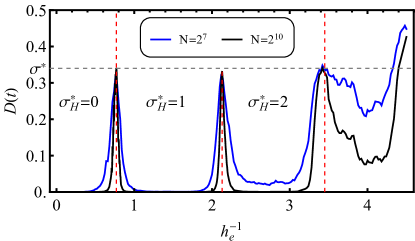
Figure 1: Long time diffusion rate of the QKR model as a function of $h_{e}^{-1}$ for $N=2^{7}$ (blue line) and $N=2^{10}$ (black line). We take ensemble average over 400 different values of $\alpha\in(0,2\pi)$ and $q\in(0,1)$. We set $t=N^{2}/4$. The transitions occur near $h_{e}=0.77$, $2.13$, and $3.45$ as indicated with red dashed lines. The diffusion rate converge to a universal value $\sigma^{*}\simeq 0.33$ (gray dashed line) at the these critical points.

The long-time diffusion rate $D(t)$ as a function of Planck’s parameter $h_{e}$ for $0\leq h_{e}^{-1}\leq 4.5$ is plotted in Fig. 1. The QKR exhibits dynamical localization with $D(t)\rightarrow 0$ as $t\rightarrow\infty$ for a generic $h_{e}$, but undergoes transitions with nonzero diffusion rate near $h_{e}=0.77$, $2.13$, and $3.45$.

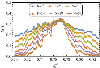
Figure 2: Long-time diffusion rate of the QKR model as a function of $h_{e}^{-1}$ near the critical point $0.77$ for various $N$. We set $t=N^{2}/4$.

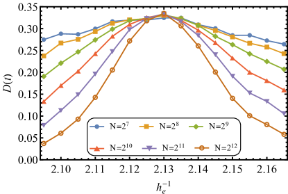
Figure 3: Long-time diffusion rate of the QKR model as a function of $h_{e}^{-1}$ near the critical point $2.13$ for various $N$. We set $t=N^{2}/4$.

III.1 Finite size scaling analysis

We then zoom in and carry out extensive simulations near $h_{e}=0.77$ and $2.13$ for various $N$ and set $t=N^{2}/4$. The results are shown in Figs. 2 and 3. We find that the data near $h_{e}=0.77$ are not quite smooth even after the ensemble average and show a bunch of peaks and dips, which might be attributed to the non-generic behavior induced by rational $h_{e}/4\pi$ Tian et al. (2011); Wang et al. (2014). We thus focus on the data near $h_{e}=2.13$.

In the long-time limit, the diffusion rate $D(t)$ goes to zero for an insulating state with dynamical localization in the momentum space, and approaches a nonzero value for a metallic state. According to the scaling theory of Anderson localization, the diffusion rate obeys the one-parameter scaling law. Near the critical point, the diffusion rate has the scaling form,

$$D(h,t)=\xi^{2-d}F(\xi^{-d}t).$$ (27)

Here $\xi$ is the localization length, which diverges as $\xi\propto|\delta h|^{-\nu}$ with $\delta h=h_{e}-h_{e,c}$. $d=2$ is the spatial dimension of the equivalent Anderson model. The truncation of the Hilbert space to $2N$-dimensional introduces a finite lattice size $2N$ in the momentum space, thus the finite-size scaling form is given by

$$D(h,t,N)=f(t/N^{2},hN^{1/\nu})\equiv f(x,y),$$ (28)

with $x=t/N^{2}$, and $y=hN^{1/\nu}$. $f$ is a non-singular function of its arguments. In the simulations, we choose $t=N^{2}/4$, thus $x=1/4$ is fixed, and expand $f$ into the power series of $y$,

$$f(x_{0},y)=\sum^{k_{\mathrm{max}}}_{k=0}a_{k}y^{k}.$$ (29)

The expansion coefficients $a_{k}$’s, the critical point $h_{e,c}$, and the critical exponent $\nu$ are free fitting parameters.

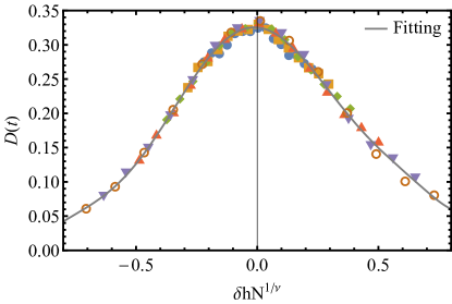
Figure 4: Data collapse of the diffusion rate $D(t)$ in Fig. 3 according to finite size scaling form in Eq. (28).

Applying the above finite-size scaling analysis, we find all data collapse onto a single smooth curve as a function of $\delta hN^{1/\nu}$ (see Fig. 4). The critical point $h_{e,c}^{-1}=2.1294(3)$, and the critical exponent $\nu=2.62(9)$. This is consistent with that of the IQH plateau transition estimated with the Chalker-Coddington model, $\nu=2.593(5)$ Chalker and Coddington (1988); Huckestein (1995); Slevin and Ohtsuki (2009), thus we confirm that the critical point of the spin-$1/2$ QKR model belongs to the universality class of the IQH plateau transitions. Moreover, we also give a precise estimate of the universal diffusion rate at the metallic critical point, $\sigma^{*}=0.3253(12)$.

IV Conclusion

To summarize, we have studied the spin-$1/2$ QKR model with extensive numerical simulations. By devising and applying the finite-size scaling analysis near the critical point between different dynamical localization phases, we obtain the numerical estimate of the critical exponent $\nu$ and the universal diffusion rate $\sigma^{*}$ at the critical point. We confirm that the transition belongs to the universality class of the IQH plateau transition.