Separated Contrastive Learning for Organ-at-Risk and Gross-Tumor-Volume Segmentation with Limited Annotation

Abstract

Automatic delineation of organ-at-risk (OAR) and gross-tumor-volume (GTV) is of great significance for radiotherapy planning. However, it is a challenging task to learn powerful representations for accurate delineation under limited pixel (voxel)-wise annotations. Contrastive learning at pixel-level can alleviate the dependency on annotations by learning dense representations from unlabeled data. Recent studies in this direction design various contrastive losses on the feature maps, to yield discriminative features for each pixel in the map. However, pixels in the same map inevitably share semantics to be closer than they actually are, which may affect the discrimination of pixels in the same map and lead to the unfair comparison to pixels in other maps. To address these issues, we propose a separated region-level contrastive learning scheme, namely SepaReg, the core of which is to separate each image into regions and encode each region separately. Specifically, SepaReg comprises two components: a structure-aware image separation (SIS) module and an intra- and inter-organ distillation (IID) module. The SIS is proposed to operate on the image set to rebuild a region set under the guidance of structural information. The inter-organ representation will be learned from this set via typical contrastive losses cross regions. On the other hand, the IID is proposed to tackle the quantity imbalance in the region set as tiny organs may produce fewer regions, by exploiting intra-organ representations. We conducted extensive experiments to evaluate the proposed model on a public dataset and two private datasets. The experimental results demonstrate the effectiveness of the proposed model, consistently achieving better performance than state-of-the-art approaches. Code is available at https://github.com/jcwang123/Separate˙CL.

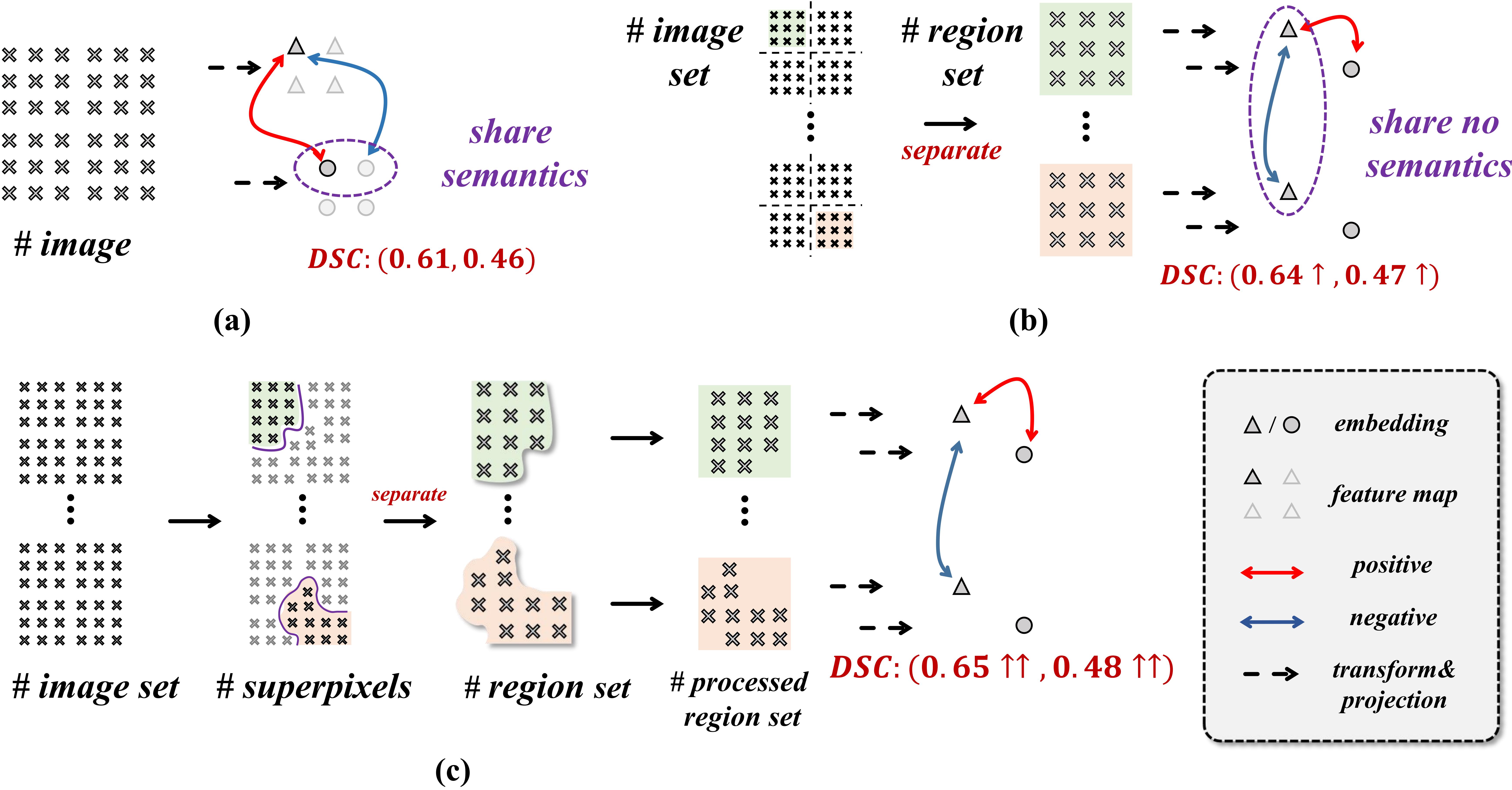
Figure 1: Motivation of building structure-aware image separation (SIS) module. (a) No separation, that forms comparison of pixels in the feature map. Pixels in the same map inevitably share semantics, which may affect the discrimination of pixels in the same map and lead to unfair comparison to pixels in other maps. (b) Regular separation, that regularly separates each image into square regions and encodes each region as a discriminative feature. Structure has been broken in the produced regions. (c) SIS, that separates each image into regions by superpixel-based division to learn their structural information. Note that the region set has been shuffled so that green region and orange region could be from different images. Evaluated DSC scores of two private datasets are shown in the figure.

Introduction

Accurate delineation of organ-at-risk (OAR) and gross-tumor-volume (GTV) in CT scans is a crucial step in radiotherapy treatment. However, manual volume delineation is one of the most time-consuming and tedious tasks for clinicians. Hence, automatic and accurate delineation tools are highly demanded in clinical practice. Recent years, researchers have proposed many deep models for medical image segmentation, such as U-Net (Ronneberger, Fischer, and Brox 2015), DenseUNet (Li et al. 2018), HyperDenseNet (Dolz et al. 2018), nnUNet (Isensee et al. 2020). Successfully training these models usually requires a large number of pixel (voxel)-wise annotations. However, in clinical practice, it is difficult, if not impossible, to acquire these annotations owing to the need of extensive professional expertise for labelling and the busy schedule of clinicians. In this regard, self-supervised learning, which attempts to learn discriminative features from a small set of labelled data and a large number of unlabeled data, becomes an important research direction in medical image segmentation.

In recent years, contrastive learning (Chen et al. 2020a, b; Grill et al. 2020; Chen and He 2020), a learning strategy that first extracts features from the unlabeled dataset and then fine-tunes the network with a few labeled images, has dominated the field of self-supervised learning. The main idea of contrastive learning is to learn representations such that make similar samples stay close to each other while dissimilar ones far apart. Nevertheless, when transferred into downstream tasks that require dense prediction, i.e., object segmentation, the representations learned by contrastive learning can only bring limited performance improvement, since it can only discriminate images rather than pixels.

Latest studies attempt to address this issue by learning discrimination of pixels in the feature maps (Chaitanya et al. 2020; Zhao et al. 2020; Xie et al. 2020; Chen et al. 2021; Alonso et al. 2021). As shown in Figure 1(a), after encoding an image into a feature map, each pixel in the map represents a square region in the image. Typical contrastive loss is then utilized to pull positive pixels together and push negative pixels far apart. These methods differ in how to determine whether a pixel is positive or negative, by pseudo label (Zhao et al. 2020; Alonso et al. 2021) or spatial distance (Chaitanya et al. 2020; Xie et al. 2020; Chen et al. 2021), yet all of them have neglected a pivotal problem that pixels in the feature map are sharing semantics, which is harmful to the pixel-level discrimination. Specifically, this issue has negative effects on both intra-image and inter-image discrimination. First, the objective of intra-image discrimination is to distinguish an anchor pixel from other pixels in the same feature map; the sharing semantics, however, make them closer. Second, the goal of inter-image discrimination is to find (dis-) similar pixels in other images, yet pixels from the same image are usually more similar than those from different images. The unfair comparison may destroy the exploration of pixel comparison cross images.

To tackle this issue, we propose a novel separated region-level contrastive learning scheme for the challenging tasks of delineation of organ-at-risk (OAR) and gross-tumor-volume (GTV) in CT scans; we call the proposed model as SepaReg. It is composed of two components: a structure-aware image separation (SIS) module and an intra- and inter-organ distillation (IID) module.

• SIS can be regarded as the core of the proposed SepaReg, in which we propose to produce a brand-new region set and learn representation from the region set instead of the image set. Regions are produced with the guidance of structural information in order to keep complete anatomical structure to enhance the recognition of boundaries. The representations are learned by performing region comparison. Besides regions from the same image, each region is compared to more regions from other images due to the separation, effectively enhancing the regional diversity.

• IID is proposed to handle the quantity imbalance that larger organs will produce more regions, which may affect the representation learning of tiny organs (Tian, Henaff, and van den Oord 2021). In IID, regions are clustered into different subsets according to their learned features; each subset represents a specific organ. The intra-organ representations are learned on each subset and distilled into one model in the end.

Extensive experiments are performed on three typical datasets, including one public dataset and two in-house datasets. The two private datasets comprise OAR segmentation for lung cancer and GTV segmentation for nasopharyngeal cancer. We compare the proposed SepaReg to several state-of-the-art image- and pixel-level contrastive learning schemes. The transfer segmentation performance on a small labeled test set is used to assess the learned representation. Experimental results demonstrate the effectiveness of the proposed model, consistently achieving better segmentation results than the state-of-the-art.

Related Work

Automatic Delineation in Radiation Therapy

A handful of studies have been proposed to address CT-based automatic segmentation of OAR and GTV in the past few years. Gradient-based image processing methods are adopted in the early years (Geets et al. 2007; Day et al. 2009; Kerhet et al. 2010). They can give coarse segmentation results on OAR whose boundary is clear to identify. While, it is still difficult to achieve satisfactory segmentation of GTV with ambiguous boundaries. Later, Deep Learning methods to perform OAR and GTV segmentation are rapidly developing and have caught lots of concentration. These models can easily obtain human-closed performance on most OARs of nasopharyngeal cancer (Ibragimov and Xing 2017), lung cancer (Zhu et al. 2019), and cervical cancer (Liu et al. 2020). As for GTV segmentation, the most popular research direction is the fusion of different modalities, such as PET and CT (Guo et al. 2019; Jin et al. 2019, 2021; Wang et al. 2020). However, models in these studies are trained under full supervision, accounting for precise annotations for each pixel (voxel). It is difficult to acquire these annotations thanks to the need of extensive professional expertise for labeling and the busy schedule of clinicians. How to improve the segmentation performance given limited annotations, is still valuable to exploit till today. With this desirable consideration, we make a comprehensive effort to introduce a quite bleeding-edge technique, contrastive learning, in the field of label-efficient OAR and GTV segmentation.

Representation Learning on CT Images

The lack of sufficient expert-annotated data for model optimization, is one of the most general problems in the medical vision field due to the expensive cost in both time and experience. Representation learning is a hot direction to solve this issue as it can help the model explore general representation from the unlabeled dataset, which can significantly improve the transfer performance on a relatively small labeled set. The representation could be learned by solving manually designed tasks, such as Jigsaw puzzle (Zhuang et al. 2019), context restoration (Taleb et al. 2020), orientation prediction (Taleb et al. 2020), or their combination (Zhou et al. 2019, 2021). Most strategies work well on 3D networks but fail in 2D area (Zhou et al. 2019), indicating the scant perception of semantic contexts in these representations. The latest work has indicated the bright future of contrastive learning, which has dominated the field of representation learning in medical image segmentation (Chaitanya et al. 2020). Despite its success in exploring global and local features, this work is still limited by the condition that all volumes should be aligned at first. Its setup for exploring pixel-level discrimination on feature maps also suffers from the sharing semantics. By contrast, SepaReg relies on no extra condition and avoids sharing semantics by its separated learning design.

Contrastive Learning for Segmentation Tasks

Contrastive learning is a successful and developing variant of representation learning, yet the investigation on segmentation tasks has not been fully studied. Current work builds this scheme by forming pixel pairs on feature maps, according to pseudo label or spatial distance. The former is not suitable when given no class label during representation learning (Zhao et al. 2020; Alonso et al. 2021), so that we mainly survey the latter. The earliest work explores local feature comparison by determining dis-similar pixels in the feature map if they are far away in spatial dimension (Chaitanya et al. 2020). Instead, PixPro ignores the dis-similar pixels and forms similar pixel pairs if they are closed (Xie et al. 2020). Considering the spatial continuity of organs in sequential or volumetric images, pixels at the same location in neighbour slices are forced to stay close (Zeng et al. 2021; Chen et al. 2021). No matter what measurement they use, these studies adopt the same design that utilizes typical contrastive loss to discriminate each pixel in the feature map. However, they have ignored a vital problem that pixels in the same feature map inevitably share semantics to affect the pixel discrimination. Our work aims to solve this issue through a separated region-level learning scheme, in which each region is encoded separately and shares no semantics.

Superpixel Segmentation

Generally, superpixel is generated by clustering local pixels using low-level image properties such as color. These methods are based on (1) graph-cut algorithms (Felzenszwalb and Huttenlocher 2004; Liu et al. 2011) that treat image as un-directed graph and partition the graph based on edge-weights, or (2) clustering algorithms (Achanta et al. 2010; Neubert and Protzel 2014; Li and Chen 2015) such as $k$-means, that are initialized by seeding pixels and use color, spatial information to update the cluster centers.

Based on superpixel, there is plenty of downstream application in medical imaging tasks (Qin et al. 2018; Jia et al. 2020; Ouyang et al. 2020; Li et al. 2020). It can be used for classification of hyperspectral images  (Jia et al. 2020), organ segmentation in CT scans (Qin et al. 2018; Ouyang et al. 2020), label softening in brain MR images (Li et al. 2020), and so on. Still, whether it is useful to introduce superpixel into the area of building dense contrastive learning has not been studied. We propose to utilize the superpixel-based division to guide the model to learn structural information to enhance segmentation performance.

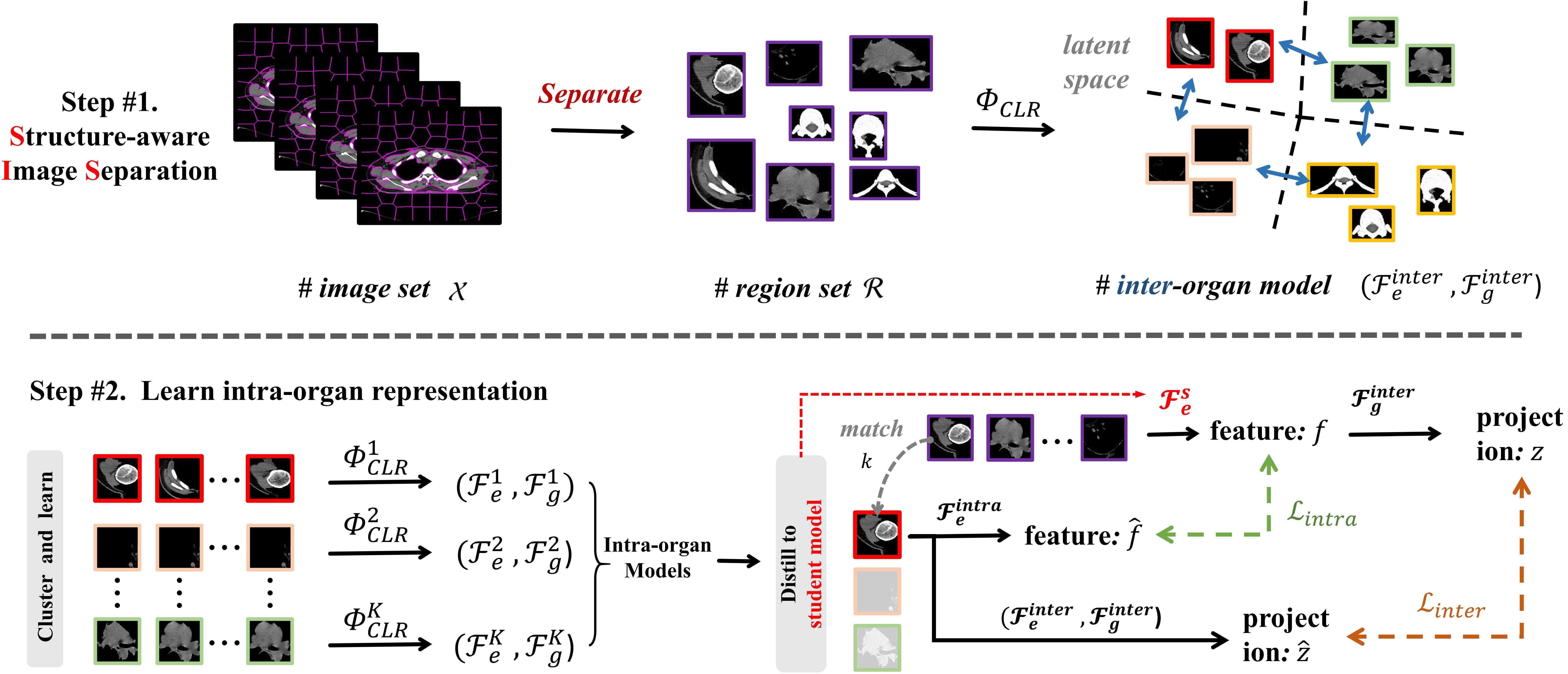
Figure 2: Framework of our separated region-level contrastive learning, SepaReg, aimed at learning region-level representation in a separated manner. It comprises two major components: a structure-aware image separation (SIS) module and an intra- and inter-organ distillation (IID) module. SIS is proposed to solve the semantics sharing, by separating each image into several regions under the guidance of structural information, to form a brand-new region set and learn regions’ representation from the set. IID is introduced to tackle the quantity imbalance in the region set since larger organ will produce more regions, by exploring intra-organ representations and distilling them into a student model. $\Phi_{CLR}$ denotes a standard contrastive learning operation, i.e., SimSiam. $\mathcal{F}_{e},\mathcal{F}_{g}$ denote the encoder and projector.

Method

In this section, we will give a detailed description of our separated learning scheme. Overall framework has also been illustrated in Figure 2. It contains two training steps, each of which will be described in an individual subsection.

Structure-aware Image Separation

Current pixel-level contrastive learning schemes encode images into feature maps and form pixel pairs in the maps. Differently, our approach starts by producing a set of regions from the image set; each region in the produced set will be embedded separately. We will describe the production in detail, followed by a brief introduction to the learning setup.

Using superpixel to separate an image into regions for unsupervised segmentation is widely adopted in previous literature (Qin et al. 2018; Ouyang et al. 2020), yet not applied into the field of contrastive learning. Specifically, let $\mathcal{F}_{s}$ denote the superpixel operation. Given an image set $\mathcal{X}$, our target is to separate it into a set of regions $\mathcal{R}$: $\mathcal{R}\leftarrow\mathcal{F}_{s}(\mathcal{X})$. Firstly, we separate each image $x$ in the image set into regions by SLIC method (Achanta et al. 2010). It begins with an initialization step where a certain number of cluster centers (set to 32 as default) are sampled on the regular grid spaced of $x$. These centers are then moved to search locations with lowest gradient in a limited neighborhood, i.e., $3\times 3$. After the moving step, an update operation is performed to adjust the cluster centers. The moving step and update operation will repeat until the new cluster centers move little, which is also similar to the $k$-means clustering algorithm. After SLIC, each region produced from image $x$ will be padded with zero value to form a new square image for subsequent learning setup. Till now, all produced regions from different images are unionized and shuffled to obtain the final region set $\mathcal{R}$.

To learn regions’ representation, we perform a standard image-level contrastive learning operation on the region set. This operation is denoted as $\Phi_{CLR}$, set to SimSiam (Chen and He 2020) as default. In formal, given a region $r$ that has been pre-processed with certain size ($128\times 128$ as default), two augmentation views $v,v^{{}^{\prime}}$ are created by different transformations $\mathcal{T},\mathcal{T}^{{}^{\prime}}$. The first augmented view $v$ is fed into an encoder $\mathcal{F}_{e}$, a standard ResNet-50 network (He et al. 2016) with removing its final two layers. The extracted feature is then projected into the projection space via a projector $\mathcal{F}_{g}$, including two layers with a hidden dimension of 4096 and output size of 256. Between the two layers, there is a sequence of Batch Normalization and Relu activation to avoid the collapsing solution (Chen and He 2020). Similarly, another augmented view $v^{{}^{\prime}}$ is fed into the encoder and projector to obtain its corresponding vector $z^{{}^{\prime}}$. An extensive predictor $\mathcal{F}_{q}$ with same architecture as projector is used to transfer $z^{{}^{\prime}}$ into $z$ by regression. The overall objective function is designed as

$$\begin{gathered}\mathcal{L}=\frac{1}{2}(\mathcal{D}(\mathcal{F}_{q}(z),z^{{}^{\prime}})+\mathcal{D}(z,\mathcal{F}_{q}(z^{{}^{\prime}})))\end{gathered}$$ (1)

Here, $\mathcal{D}$ is used to measure the cosine similarity in the projection space, as

$$\mathcal{D}(\mathcal{F}_{q}(z),z^{{}^{\prime}})=-\frac{\mathcal{F}_{q}(z)}{||\mathcal{F}_{q}(z)||_{2}}\cdot\frac{z^{{}^{\prime}}}{||z^{{}^{\prime}}||_{2}},$$ (2)

where $||\cdot||_{2}$ is $l_{2}$-norm. The error $\mathcal{L}$ is calculated for each region and the total loss is averaged on all regions in a mini-batch. As learned representation can coarsely discriminate different organs, we refer to it as the inter-organ model: $(\mathcal{F}_{e}^{inter},\mathcal{F}_{g}^{inter})$.

Learn Intra-organ Representation

In this part, we extensively present a distillation-based module to solve the quantity imbalance by learning intra-organ representations. As the inter-organ model can tell semantic difference of organs, we propose to cluster the region set into several subsets according to what organs they are from. For each organ, we will learn its specific representation by performing $\Phi_{CLR}$ on its corresponding subset so that tiny organs’ representations could be learned well. After that, we distill all intra-organ representations and the inter-organ representation into a student model.

Formally, we cluster the region set into $K$ (empirically set to 5 as default) subsets according to their projection by $(\mathcal{F}_{e}^{inter},\mathcal{F}_{g}^{inter})$ based on $k$-means method, that are $\mathcal{R}^{1,2...K}$. For each subset, we will train a new encoder from scratch using the operator $\Phi_{CLR}$ to learn its intra-organ representation. In total, $K$ encoders will be trained at this stage, and we denote these intra-organ models as $\{(\mathcal{F}_{e}^{k},\mathcal{F}_{g}^{k})|k=1,2...K\}$.

The distillation module is trained under intra-organ and inter-organ regularization. As shown in Figure 2, it contains two parts: (1) For intra-organ regularization, given a region $r$ from the region set $\mathcal{R}$, the organ it belongs to could be matched, as well as the intra-organ model corresponding to it. By feeding this region into the encoder of its intra-organ model, $\mathcal{F}_{e}^{intra}$, we could obtain the feature $\hat{f}$ that the student model should learn from. We minimize the $KL$-divergence error between two features:

$$\mathcal{L}_{intra}=KL~{}(f~{}||~{}\hat{f}),$$ (3)

where $f$ is the feature encoded by the student model. (2) For the inter-organ regularization, telling the discrimination between different organs is more important to learn. Therefore, we first feed the region into the inter-organ model to get its projection $\hat{z}$, then use the inter-organ projector to project $f$ into latent space and let the projection consistent with $\hat{z}$. The objective function is defined as

$$\mathcal{L}_{inter}=\mathcal{D}~{}(\mathcal{F}_{g}^{chair}(f)~{},~{}\hat{z}),$$ (4)

where $\mathcal{D}$ is the same measurement as Eq.2.

In summary, $\mathcal{L}_{intra}$ is used to tell organ-specific feature representation and $\mathcal{L}_{inter}$ is used to learn the discriminative relation between different organs. We combine these two constraints to train our distillation network, that is,

$$\mathcal{L}_{distill}~{}=~{}\mathcal{L}_{intra}~{}+~{}\mathcal{L}_{inter}~{}.$$ (5)

After distillation, we initialize a standard U-Net’s encoder with the pretrained weight, followed by using Dice loss to optimize the parameters of the entire model.

Method	DSC$\uparrow$			HD95$\downarrow$
	$|X_{tr}|=1$	$|X_{tr}|=10$	$|X_{tr}|=50$	$|X_{tr}|=1$	$|X_{tr}|=10$	$|X_{tr}|=50$
Random Init.	$61.26\pm 0.55$	$78.34\pm 0.12$	$82.03\pm 0.09$	$6.49\pm 6.94$	$2.48\pm 0.22$	$2.01\pm 0.16$
SimCLR (Chen et al. 2020a)	$63.03\pm 0.86$	$80.88\pm 0.13$	$83.61\pm 0.08$	$4.41\pm 2.71$	$2.07\pm 0.10$	$1.80\pm 0.18$
BYOL (Grill et al. 2020)	$61.66\pm 0.61$	$80.00\pm 0.11$	$82.90\pm 0.09$	$5.12\pm 2.42$	$2.35\pm 0.16$	$1.91\pm 0.27$
SimSiam (Chen and He 2020)	$61.67\pm 0.68$	$79.68\pm 0.11$	$83.16\pm 0.09$	$5.34\pm 5.08$	$2.22\pm 0.20$	$1.92\pm 0.36$
GL (Chaitanya et al. 2020)	$61.64\pm 0.79$	$80.11\pm 0.12$	$82.60\pm 0.09$	$6.04\pm 5.84$	$2.28\pm 0.15$	$1.84\pm 0.21$
PixPro (Xie et al. 2020)	$65.34\pm 0.51$	$79.65\pm 0.12$	$83.11\pm 0.07$	$5.13\pm 3.58$	$2.39\pm 0.35$	$1.87\pm 0.21$
SepaReg	$66.27\pm 0.50$	$81.59\pm 0.13$	$83.71\pm 0.09$	$4.05\pm 2.73$	$1.90\pm 0.13$	$1.69\pm 0.25$

Table 1: Comparison results on our private dataset, LungOAR, with state-of-the-art contrastive learning methods, including image-level and pixel-level methods. ”Random Init.” means training from scratch. We show the DSC score (%) and HD95 value (voxel) as well as the standard error in patient-wise.

Method	DSC$\uparrow$			HD95$\downarrow$
	$|X_{tr}|=1$	$|X_{tr}|=10$	$|X_{tr}|=50$	$|X_{tr}|=1$	$|X_{tr}|=10$	$|X_{tr}|=50$
Random Init.	$42.87\pm 2.62$	$55.28\pm 3.19$	$61.05\pm 2.61$	$12.90\pm 55.33$	$8.90\pm 39.58$	$11.11\pm 234.00$
SimCLR (Chen et al. 2020a)	$47.41\pm 2.98$	$58.71\pm 2.51$	$62.46\pm 2.94$	$12.96\pm 45.53$	$8.52\pm 32.17$	$7.36\pm 29.96$
BYOL (Grill et al. 2020)	$47.23\pm 2.94$	$59.01\pm 2.54$	$63.62\pm 2.81$	$12.81\pm 52.39$	$8.23\pm 28.98$	$7.32\pm 31.35$
SimSiam (Chen and He 2020)	$46.06\pm 2.94$	$58.34\pm 2.76$	$63.45\pm 2.73$	$14.81\pm 56.71$	$8.28\pm 32.54$	$7.34\pm 26.18$
GL (Chaitanya et al. 2020)	$48.30\pm 2.71$	$59.06\pm 2.91$	$61.88\pm 2.59$	$13.70\pm 85.04$	$8.25\pm 32.44$	$7.25\pm 31.66$
PixPro (Xie et al. 2020)	$48.52\pm 2.82$	$57.18\pm 2.72$	$60.79\pm 2.44$	$12.92\pm 53.45$	$9.40\pm 40.74$	$8.00\pm 30.12$
SepaReg	$50.30\pm 2.12$	$60.03\pm 2.33$	$63.98\pm 2.06$	$12.31\pm 44.06$	$7.54\pm 33.18$	$6.77\pm 30.27$

Table 2: Comparison results on our private dataset, NasoGTV, with state-of-the-art contrastive learning methods, including image-level and pixel-level methods. ”Random Init.” means training from scratch. We show the DSC score (%) and HD95 value (voxel) as well as the standard error in patient-wise.

Method	All OARs	SMG		Parotid		Brain Stem	Mandible
		Lt	Rt	Lt	Rt
Random Init.	$54.48\pm 0.35$	$38.61\pm 3.99$	$25.03\pm 2.27$	$58.34\pm 0.18$	$63.06\pm 0.38$	$64.45\pm 2.15$	$77.38\pm 0.19$
SimCLR	$57.10\pm 0.22$	$33.45\pm 5.98$	$21.81\pm 2.15$	$62.30\pm 0.34$	$68.23\pm 0.25$	$75.11\pm 0.28$	$81.71\pm 0.16$
BYOL	$57.34\pm 0.27$	$40.21\pm 6.49$	$25.32\pm 0.86$	$59.40\pm 0.56$	$66.84\pm 0.33$	$73.63\pm 0.61$	$78.65\pm 0.32$
SimSiam	$54.83\pm 0.14$	$33.25\pm 6.57$	$25.78\pm 2.54$	$65.79\pm 0.23$	$56.63\pm 0.87$	$68.25\pm 1.38$	$79.27\pm 0.23$
GL	$52.03\pm 0.12$	$44.06\pm 2.54$	$6.01\pm 0.35$	$54.34\pm 0.28$	$61.39\pm 0.45$	$65.05\pm 0.79$	$81.30\pm 0.20$
PixPro	$51.12\pm 0.65$	$37.78\pm 5.04$	$18.40\pm 1.57$	$48.95\pm 2.19$	$59.00\pm 2.07$	$62.26\pm 1.65$	$80.33\pm 0.26$
SepaReg	$58.43\pm 0.10$	$45.29\pm 5.98$	$27.99\pm 1.55$	$58.42\pm 0.35$	$67.65\pm 0.16$	$73.58\pm 0.42$	$77.64\pm 0.33$

Table 3: Comparison results on a small public dataset, PDDCA, with state-of-the-art contrastive learning methods, including image-level and pixel-level methods. We report the results when $|X_{tr}|=1$ as there is little available data. ”Random Init.” means training from scratch. We show the DSC score (%) and standard error of each organ as well as the averaged value on all OARs in patient-wise.

Experiments

Datasets

We compare our method with several state-of-the-art contrastive learning methods on three CT datasets, including one public dataset and two in-house clinical datasets.

PDDCA is a public dataset consisting of 32 Head&Neck CT scans with six OAR segmentation labels, i. e., submandibular gland (left and right), parotid (left and right), brain stem, and mandible (Raudaschl et al. 2017). However, the dataset is a bit small, lacks concrete and consistent annotations. Hence, we also collect two larger clinical datasets to validate the performance of our method.

LungOAR is a clinical dataset, collected by Philips scanner in a local hospital. It contains 97 volumes and the target of this dataset is to segment the esophagus of lung cancer. For the annotation, one junior radiologist helps the first-round annotations, and one senior radiologist helps the second-round check to ensure accuracy. All data has been anonymized, and we have received approval from local hospitals for research purposes.

NasoGTV is a clinical dataset, consisting of 93 volumes. The images are collected by the CMS scanner. The target of this dataset is to segment the GTV of nasopharyngeal carcinoma. The same annotation process is performed by local radiologists and we have also received the approval.

Experimental Setup and Comparison

Pretrain stage

Following (Chaitanya et al. 2020), we split each dataset into a pre-training set $X_{pre}$ and a test set $X_{ts}$, where the volumetric images in $X_{pre}$ are used for pre-training, and those in $X_{ts}$ are only used to assess the segmentation performance. We randomly choose 77, 73, 22 volumes to form $X_{pre}$ for LungOAR dataset, NasoGTV dataset and PDDCA dataset, respectively. The rest of volumes in each dataset will be used to form the test set.

Finetune stage

As for the stage of fine-tuning, we choose a certain number of samples out of $X_{pre}$, consisting of both volumetric images and segmentation labels, to form the training set $X_{tr}$ and the validation set $X_{vl}$, where $|X_{vl}|=7$ in LungOAR, $|X_{vl}|=3$ in NasoGTV, and $|X_{vl}|=2$ in PDDCA. We experiment with different sizes of $X_{tr}$ to assess the pre-trained representation. For instance, in LungOAR and NasoGTV, we build three experiments with $|X_{tr}|=1,10,50$. PDDCA is so small that we only test the transfer performance with $|X_{tr}=1|$.

We compare our method to several contrastive learning methods: (I) image-level methods: SimCLR (Chen et al. 2020a), BYOL (Grill et al. 2020), SimSiam (Chen and He 2020). (II) region-level methods: the scheme exploring global and local features, dubbed GL (Chaitanya et al. 2020), and PixPro (Xie et al. 2020). ResNet-50 and standard U-Net are used in all these experiments, and we implement these methods on three datasets by using the official code. We pre-train all the models for 100k iterations in total, and each mini-batch contains 32 images/regions. As for finetuning, we train the model for 200 epochs in all settings, save the best model of the validation set, and evaluate it on the test set in the end. Dice similarity coefficient (DSC) and 95% Hausdorff Distance (HD95) are used to evaluate the segmentation performance at the patient level.

Comparison with the State-of-the-Art Methods

Table 1 shows the results of our method on LungOAR dataset. We can observe: (1) contrastive learning indeed brings improvements. Compared with ”Random Init.”, it is found that all methods have given better DSC score and HD95 value, and the improvement is larger with a smaller labeled set. (2) our method outperforms other methods with $1\%\sim 2\%$ improvement on DSC score when $|X_{tr}|=1,10$, and has also better result when $|X_{tr}|=50$. For example, when $|X_{tr}|=1$, our methods have improved the DSC score by $5.01\%$, which is significantly larger than the image-level method, i.e. $1.77\%$ by SimCLR, also obviously larger than region-level method, i.e., $4.08\%$ by PixPro. (3) it is also noteworthy that PixPro can outperform other image-level contrastive learning methods when $|X_{tr}|=1$, while show inferior results when enlarging the training set. It indicates that the representation learned by PixPro is not suitable for the downstream segmentation task. In contrast, our method brings larger improvement even when $|X_{tr}|=50$.

As shown in Table 2, the results on NasoGTV keep consistent with those from Table 1, validating the effectiveness of our method to extract self-learned features for the segmentation task. Since GTV segmentation is more challenging than OAR segmentation, we note that our method achieves outstanding improvements.

Table 3 summarizes the results on PDDCA dataset. We can observe the best average score of all OARs achieved by our method. The results further indicate the robustness of our method. It is noteworthy that GL and PixPro yield worse segmentation results compared to the random initialization. This is because organs in this dataset have no square shape, i.e., parotid that is spindly, leading to mistakes in obtaining the region pairs. Instead, our proposed separated learning scheme can take advantage of structural information and thus enable the network to learn shape-adaptive knowledge.

	LungOAR	NasoGTV
no separation	$60.63\pm 0.97$	$46.22\pm 2.58$
regular separation	$63.78\pm 0.69$	$47.14\pm 2.91$
SIS	$65.32\pm 0.48$	$48.41\pm 2.79$

Table 4: Comparison of different separation strategies: no separation, regular separation, and structure-aware separation (SIS). We report the DSC score (%) and standard error in patient-wise.

SIS	IID	LungOAR	NasoGTV
		$61.26\pm 0.55$	$42.87\pm 2.62$
✓		$65.32\pm 0.48$	$48.41\pm 2.79$
✓	✓	$66.27\pm 0.50$	$50.30\pm 2.12$

Table 5: Ablation study of SIS and IID. The first row with no modules denotes training with random initialization. The combination of SIS and IID, is our separated region-level contrastive learning scheme, SepaReg. We report the DSC value (%) and standard error in patient-wise.

$\mathcal{L}_{intra}$	$\mathcal{L}_{inter}$	LungOAR	NasoGTV
		$65.32\pm 0.48$	$48.41\pm 2.79$
✓		$65.80\pm 0.65$	$48.79\pm 2.82$
✓	✓	$66.27\pm 0.50$	$50.30\pm 2.12$

Table 6: Analytical study of two objectives in our distillation network. Basic scheme without any objectives is the separate learning scheme using superpixel method.

Ablation Study

In this part, we analyze the effectiveness of each module in our method. For simplification, we only present the DSC score when $|X_{tr}|=1$.

How important the structure-aware separation is?

As shown in Table 4, we first compare with three learning schemes to verify the effectiveness of superpixel-based separable feature extraction. They have also been visualized in Figure 1, and the result has been shown in Table 4. No separation refers to form positive region pairs at the same location of two feature maps. It can be regarded as PixPro with removing its PPM module. Regular separation refer to separate each image into regular grid regions, and SIS is the structure-aware image separation. We can see that the separation can improve transfer segmentation performance, demonstrating the effectiveness of separating the feature extraction. SIS extensively increases the DSC scores, indicating that structural-aware separation can extract structural information for better segmentation.

How do two major components affect?

SepaReg is composed of two major parts, and we make an analytical study about their influence in Table 5. Firstly, compared to the model trained from scratch, it is observed that the SIS has already yielded good segmentation improvement. The DSC value has been improved by $4.06\%$ and $5.54\%$, indicating the powerful ability in learning region-level representation. Secondly, after learning intra-organ representations, the transfer performance reaches the best, since IID can break the quantity imbalance between regions of different organs.

Design of intra- and inter-organ distillation.

We conduct an ablation experiment about these two objectives of IID, $\mathcal{L}_{intra}$ and $\mathcal{L}_{inter}$, in Table 6. It could be seen that constraints from the intra-organ models can significantly improve the transfer performance and constraint from inter-organ model can further improve it, demonstrating the complementary advantage of both objectives.

Other Analysis

How does training iteration matter?

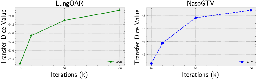
Figure 3: The transfer performance of models pre-trained at different amount of iterations on OAR and GTV datasets (left: LungOAR; right: NasoGTV).

Dividing images into regions can help the model learn to discriminate different regions. Still, it needs more iterations to update the parameters, as one mini-batch of regions contains much less information than that of images. We evaluate the transfer segmentation performance of pretrained weights at different iterations, i.e. 10k, 50k and 100k. According to the result in Figure 3, it is observed that when trained at a small number of iterations, SIS performs not so good. While meeting more samples and trained at larger iterations, the performance grows to the best.

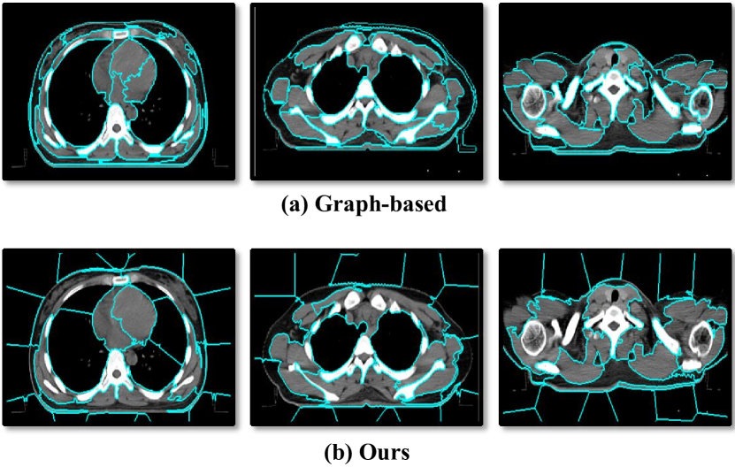
Figure 4: Regions in lung CT scans produced by (a) gragh-based superpixel method, and (b) our method. It’s found that the gragh-based method can produce regions that best fit the boundary but have large variety in shape and size, not suitable for subsequent learning scheme. Regions produced by our method have more regular shape and can also provide complete structural information to discriminate different organs, i.e., lung and heart.

Different superpixel methods.

SIS applies a cluster-based superpixel method to guide the image separation. However, some work argues that using the graph-based method can represent the structural information better (Ouyang et al. 2020). We give several typical results generated by two types of superpixel methods in Figure 4. It is found that the graph-based methods can yield regions that fit the boundary better than our produced regions. Despite it, regions created by the graph-based method have more irregular shapes and sizes at the same time, not suitable for subsequent learning schemes.

SepaReg	M&T	LungOAR	NasoGTV
✓		$66.27\pm 0.50$	$50.30\pm 2.12$
	✓	$62.92\pm 0.48$	$45.19\pm 2.58$
✓	✓	$67.11\pm 0.30$	$50.80\pm 2.80$

Table 7: Extensive experiment about the comparison of SepaReg and Mean Teacher (M&T). Here, we report the DSC score (%) and standar error in patient-wise.

Combination with semi-supervised method.

Contrastive learning aims to provide suitable initialized parameters for better transfer performance on a small amount of labeled data. With the same goal, semi-supervised method, i.e., Mean Teacher, is also helpful. In this part, we make an extensive experiment to verify two points: (i) SepaReg can give better segmentation performance on limited labeled data, (ii) SepaReg and Mean Teacher can provide complementary information to boost the segmentation performance further. Specifically, we construct this experiment on both datasets with $|X_{tr}|=1$. The same unlabeled dataset is used for Mean Teacher (M&T) training ($X_{pre}$). We combine SepaReg and M&T by initializing the ”Teacher-Student” model in M&T with parameters trained by SepaReg. It is found that (1) on both datasets, SepaReg outperforms Mean Teacher significantly, i.e. $3.35\%$ and $5.11\%$ improvements on DSC sore, and (2) the combination can further improve the DSC scores, indicating the valuable potential of their complementary information.

Conclusion

In this paper, we devise a separated region-level contrastive learning scheme, named SepaReg, to solve the problem of sharing semantics in latest pixel-level contrastive learning schemes. SepaReg comprises two components: structure-aware image separation (SIS) and intra- and inter-organ distillation module (IID). SIS proposes to produce a brand-new region set by separating each image into regions under the guidance of structural information, and learn their representations by forming region comparison. IID is proposed to boost the representation learning of tiny organs, since tiny organs produce few regions in the set, by exploring inra-organ representations. SepaReg is evaluated on one public dataset and two clinical datasets, achieving the best DSC score and HD95 value on all test sets, compared to several image- and pixel-level contrastive learning methods.

References

- Achanta et al. (2010) Achanta, R.; Shaji, A.; Smith, K.; Lucchi, A.; Fua, P.; and Süsstrunk, S. 2010. Slic superpixels. Technical report.
- Alonso et al. (2021) Alonso, I.; Sabater, A.; Ferstl, D.; Montesano, L.; and Murillo, A. C. 2021. Semi-Supervised Semantic Segmentation with Pixel-Level Contrastive Learning from a Class-wise Memory Bank. arXiv preprint arXiv:2104.13415.
- Chaitanya et al. (2020) Chaitanya, K.; Erdil, E.; Karani, N.; and Konukoglu, E. 2020. Contrastive learning of global and local features for medical image segmentation with limited annotations. Advances in Neural Information Processing Systems, 33.
- Chen et al. (2020a) Chen, T.; Kornblith, S.; Norouzi, M.; and Hinton, G. 2020a. A simple framework for contrastive learning of visual representations. In International conference on machine learning, 1597–1607. PMLR.
- Chen et al. (2020b) Chen, T.; Kornblith, S.; Swersky, K.; Norouzi, M.; and Hinton, G. 2020b. Big self-supervised models are strong semi-supervised learners. arXiv preprint arXiv:2006.10029.
- Chen and He (2020) Chen, X.; and He, K. 2020. Exploring Simple Siamese Representation Learning. arXiv preprint arXiv:2011.10566.
- Chen et al. (2021) Chen, Z.; Zhuo, W.; Wang, T.; Xue, W.; and Ni, D. 2021. Bootstrap Representation Learning for Segmentation on Medical Volumes and Sequences. arXiv preprint arXiv:2106.12153.
- Day et al. (2009) Day, E.; Betler, J.; Parda, D.; Reitz, B.; Kirichenko, A.; Mohammadi, S.; and Miften, M. 2009. A region growing method for tumor volume segmentation on PET images for rectal and anal cancer patients. Medical physics, 36(10): 4349–4358.
- Dolz et al. (2018) Dolz, J.; Gopinath, K.; Yuan, J.; Lombaert, H.; Desrosiers, C.; and Ayed, I. B. 2018. HyperDense-Net: a hyper-densely connected CNN for multi-modal image segmentation. IEEE transactions on medical imaging, 38(5): 1116–1126.
- Felzenszwalb and Huttenlocher (2004) Felzenszwalb, P. F.; and Huttenlocher, D. P. 2004. Efficient graph-based image segmentation. International journal of computer vision, 59(2): 167–181.
- Geets et al. (2007) Geets, X.; Lee, J. A.; Bol, A.; Lonneux, M.; and Grégoire, V. 2007. A gradient-based method for segmenting FDG-PET images: methodology and validation. European journal of nuclear medicine and molecular imaging, 34(9): 1427–1438.
- Grill et al. (2020) Grill, J.-B.; Strub, F.; Altché, F.; Tallec, C.; Richemond, P. H.; Buchatskaya, E.; Doersch, C.; Pires, B. A.; Guo, Z. D.; Azar, M. G.; et al. 2020. Bootstrap your own latent: A new approach to self-supervised learning. arXiv preprint arXiv:2006.07733.
- Guo et al. (2019) Guo, Z.; Guo, N.; Gong, K.; Li, Q.; et al. 2019. Gross tumor volume segmentation for head and neck cancer radiotherapy using deep dense multi-modality network. Physics in Medicine & Biology, 64(20): 205015.
- He et al. (2016) He, K.; Zhang, X.; Ren, S.; and Sun, J. 2016. Deep residual learning for image recognition. In Proceedings of the IEEE conference on computer vision and pattern recognition, 770–778.
- Ibragimov and Xing (2017) Ibragimov, B.; and Xing, L. 2017. Segmentation of organs-at-risks in head and neck CT images using convolutional neural networks. Medical physics, 44(2): 547–557.
- Isensee et al. (2020) Isensee, F.; Jaeger, P. F.; Kohl, S. A.; Petersen, J.; and Maier-Hein, K. H. 2020. nnU-Net: a self-configuring method for deep learning-based biomedical image segmentation. Nature Methods, 1–9.
- Jia et al. (2020) Jia, S.; Deng, X.; Xu, M.; Zhou, J.; and Jia, X. 2020. Superpixel-Level Weighted Label Propagation for Hyperspectral Image Classification. IEEE Transactions on Geoscience and Remote Sensing, 58(7): 5077–5091.
- Jin et al. (2019) Jin, D.; Guo, D.; Ho, T.-Y.; Harrison, A. P.; Xiao, J.; Tseng, C.-K.; and Lu, L. 2019. Accurate esophageal gross tumor volume segmentation in pet/ct using two-stream chained 3d deep network fusion. In International Conference on Medical Image Computing and Computer-Assisted Intervention, 182–191. Springer.
- Jin et al. (2021) Jin, D.; Guo, D.; Ho, T.-Y.; Harrison, A. P.; Xiao, J.; Tseng, C.-K.; and Lu, L. 2021. DeepTarget: Gross tumor and clinical target volume segmentation in esophageal cancer radiotherapy. Medical Image Analysis, 68: 101909.
- Kerhet et al. (2010) Kerhet, A.; Small, C.; Quon, H.; Riauka, T.; Schrader, L.; Greiner, R.; Yee, D.; McEwan, A.; and Roa, W. 2010. Application of machine learning methodology for PET-based definition of lung cancer. Current oncology, 17(1): 41.
- Li et al. (2020) Li, H.; Wei, D.; Cao, S.; Ma, K.; Wang, L.; and Zheng, Y. 2020. Superpixel-Guided Label Softening for Medical Image Segmentation. In International Conference on Medical Image Computing and Computer-Assisted Intervention, 227–237. Springer.
- Li et al. (2018) Li, X.; Chen, H.; Qi, X.; Dou, Q.; Fu, C.-W.; and Heng, P.-A. 2018. H-DenseUNet: hybrid densely connected UNet for liver and tumor segmentation from CT volumes. IEEE transactions on medical imaging, 37(12): 2663–2674.
- Li and Chen (2015) Li, Z.; and Chen, J. 2015. Superpixel segmentation using linear spectral clustering. In Proceedings of the IEEE Conference on Computer Vision and Pattern Recognition, 1356–1363.
- Liu et al. (2011) Liu, M.-Y.; Tuzel, O.; Ramalingam, S.; and Chellappa, R. 2011. Entropy rate superpixel segmentation. In CVPR 2011, 2097–2104. IEEE.
- Liu et al. (2020) Liu, Z.; Liu, X.; Xiao, B.; Wang, S.; Miao, Z.; Sun, Y.; and Zhang, F. 2020. Segmentation of organs-at-risk in cervical cancer CT images with a convolutional neural network. Physica Medica, 69: 184–191.
- Neubert and Protzel (2014) Neubert, P.; and Protzel, P. 2014. Compact watershed and preemptive slic: On improving trade-offs of superpixel segmentation algorithms. In 2014 22nd international conference on pattern recognition, 996–1001. IEEE.
- Ouyang et al. (2020) Ouyang, C.; Biffi, C.; Chen, C.; Kart, T.; Qiu, H.; and Rueckert, D. 2020. Self-supervision with Superpixels: Training Few-Shot Medical Image Segmentation Without Annotation. In European Conference on Computer Vision, 762–780. Springer.
- Qin et al. (2018) Qin, W.; Wu, J.; Han, F.; Yuan, Y.; Zhao, W.; Ibragimov, B.; Gu, J.; and Xing, L. 2018. Superpixel-based and boundary-sensitive convolutional neural network for automated liver segmentation. Physics in Medicine & Biology, 63(9): 095017.
- Raudaschl et al. (2017) Raudaschl, P. F.; Zaffino, P.; Sharp, G. C.; Spadea, M. F.; Chen, A.; Dawant, B. M.; Albrecht, T.; Gass, T.; Langguth, C.; Lüthi, M.; et al. 2017. Evaluation of segmentation methods on head and neck CT: auto-segmentation challenge 2015. Medical physics, 44(5): 2020–2036.
- Ronneberger, Fischer, and Brox (2015) Ronneberger, O.; Fischer, P.; and Brox, T. 2015. U-net: Convolutional networks for biomedical image segmentation. In International Conference on Medical image computing and computer-assisted intervention, 234–241. Springer.
- Taleb et al. (2020) Taleb, A.; Loetzsch, W.; Danz, N.; Severin, J.; Gaertner, T.; Bergner, B.; and Lippert, C. 2020. 3D Self-Supervised Methods for Medical Imaging. arXiv preprint arXiv:2006.03829.
- Tian, Henaff, and van den Oord (2021) Tian, Y.; Henaff, O. J.; and van den Oord, A. 2021. Divide and Contrast: Self-supervised Learning from Uncurated Data. arXiv:2105.08054.
- Wang et al. (2020) Wang, X.; Yang, G.; Zhang, Y.; Zhu, L.; and Dai, Z. 2020. Automated delineation of nasopharynx gross tumor volume for nasopharyngeal carcinoma by plain CT combining contrast-enhanced CT using deep learning. Journal of Radiation Research and Applied Sciences, 13(1): 568–577.
- Xie et al. (2020) Xie, Z.; Lin, Y.; Zhang, Z.; Cao, Y.; Lin, S.; and Hu, H. 2020. Propagate Yourself: Exploring Pixel-Level Consistency for Unsupervised Visual Representation Learning. arXiv preprint arXiv:2011.10043.
- Zeng et al. (2021) Zeng, D.; Wu, Y.; Hu, X.; Xu, X.; Yuan, H.; Huang, M.; Zhuang, J.; Hu, J.; and Shi, Y. 2021. Positional Contrastive Learning for Volumetric Medical Image Segmentation. arXiv preprint arXiv:2106.09157.
- Zhao et al. (2020) Zhao, X.; Vemulapalli, R.; Mansfield, P.; Gong, B.; Green, B.; Shapira, L.; and Wu, Y. 2020. Contrastive Learning for Label-Efficient Semantic Segmentation. arXiv preprint arXiv:2012.06985.
- Zhou et al. (2021) Zhou, Z.; Sodha, V.; Pang, J.; Gotway, M. B.; and Liang, J. 2021. Models Genesis. Medical Image Analysis, 67: 101840.
- Zhou et al. (2019) Zhou, Z.; Sodha, V.; Rahman Siddiquee, M. M.; Feng, R.; Tajbakhsh, N.; Gotway, M. B.; and Liang, J. 2019. Models Genesis: Generic Autodidactic Models for 3D Medical Image Analysis. 384–393. Cham: Springer International Publishing. ISBN 978-3-030-32251-9.
- Zhu et al. (2019) Zhu, J.; Zhang, J.; Qiu, B.; Liu, Y.; Liu, X.; and Chen, L. 2019. Comparison of the automatic segmentation of multiple organs at risk in CT images of lung cancer between deep convolutional neural network-based and atlas-based techniques. Acta Oncologica, 58(2): 257–264.
- Zhuang et al. (2019) Zhuang, X.; Li, Y.; Hu, Y.; Ma, K.; Yang, Y.; and Zheng, Y. 2019. Self-supervised feature learning for 3d medical images by playing a rubik’s cube. In International Conference on Medical Image Computing and Computer-Assisted Intervention, 420–428. Springer.