On the extreme eigenvalues and asymptotic conditioning of a class of Toeplitz matrix-sequences arising from fractional problems

Abstract

The analysis of the spectral features of a Toeplitz matrix-sequence $\left\{T_{n}(f)\right\}_{n\in\mathbb{N}}$, generated by a symbol $f\in L^{1}([-\pi,\pi])$, real-valued almost everywhere (a.e.), has been provided in great detail in the last century, as well as the study of the conditioning, when $f$ is nonnegative a.e. Here we consider a novel type of problem arising in the numerical approximation of distributed-order fractional differential equations (FDEs), where the matrices under consideration take the form

$$\mathcal{T}_{n}=c_{0}T_{n}(f_{0})+c_{1}h^{h}T_{n}(f_{1})+c_{2}h^{2h}T_{n}(f_{2})+\cdots+c_{n-1}h^{(n-1)h}T_{n}(f_{n-1}),$$

$c_{0},c_{1},\ldots,c_{n-1}\in[c_{*},c^{*}]$, $c^{*}\geqslant c_{*}>0$, independent of $n$, $h=\frac{1}{n}$, $f_{j}\sim g_{j}$, $g_{j}=|\theta|^{2-jh}$, $j=0,\ldots,n-1$. Since the resulting generating function depends on $n$, the standard theory cannot be applied and the analysis has to be performed using new ideas. Few selected numerical experiments are presented, also in connection with matrices that come from distributed-order FDE problems, and the adherence with the theoretical analysis is discussed together with open questions and future investigations.

Keywords: Toeplitz sequences; algebra of matrix-sequences; generating function; fractional operators.

AMS SC: 15B05; 15A18; 26A33

1 Introduction

In many practical applications it is required to solve numerically linear systems of Toeplitz kind and of (very) large dimensions and hence several specialized techniques of iterative type, such as preconditioned Krylov methods and ad hoc multigrid procedures have been designed; we refer the interested reader to the books [4, 14] and to the references therein. We recall that such types of large Toeplitz linear systems emerge from specific applications involving e.g. the numerical solution of (integro-) differential equations and of problems with Markov chains. On the other hand, quite recently, new examples of real world problems have emerged and among them we can cite the modeling of anomalous diffusion processes, which naturally lead to the use of fractional differential equations (FDEs). Also in this case we encounter Toeplitz structures, which are dense since the fractional operators are inherently nonlocal and hence new numerical challenges have come into the play. In all the considered applications, the sizes of resulting matrices are large and iterative solvers have to be considered, both for numerical stability and computational issues. The convergence analysis of such iterative procedures can be performed when we know the spectral features of the considered coefficient matrices. This has been done in the recent literature for certain constant-order FDE problems (see, e.g., [6, 7]), by exploiting the well-established analysis of the spectral features of Toeplitz matrix-sequences generated by Lebesgue integrable functions and the more recent Generalized Locally Toeplitz theory [9].

Here we consider a novel type of problem arising in the numerical approximation of distributed-order fractional operators. The latter can be interpreted as a parallel distribution of derivatives of fractional orders, whose most immediate application consists in the physical modeling of systems characterized by a superposition of different processes operating in parallel. As an example, we mention the application of fractional distributed-order operators as a tool for accounting memory effects in composite materials [3] or multi-scale effects [2]. For a detailed review on the topic we refer the reader to [5]. The procedure to numerically approximate distributed-order operators is made of two steps: 1) as the distributed-order operator consists of a continuous distribution of fractional order, a numerical integration is used to discretize the distributed-order operator into a multi-term constant-order fractional derivative; 2) following the conversion of the distributed-order operator into a multi-term fractional derivative, an approximation method has to be used for discretizing each constant-order fractional derivative composing the multi-term derivative.

In this paper, we focus on the case left open in [13] which arises when the integral partition width used in step 1) is asymptotic to the discretization step adopted in 2) and where the matrices under consideration take the form

$$\mathcal{T}_{n}\mathrel{\mathop{\ordinarycolon}}=c_{0}T_{n}(f_{0})+c_{1}h^{h}T_{n}(f_{1})+c_{2}h^{2h}T_{n}(f_{2})+\cdots+c_{n-1}h^{(n-1)h}T_{n}(f_{n-1}),$$ (1)

where $T_{n}(f_{j})$ is the Toeplitz matrix of size $n$ generated by $f_{j}$, the constants $c_{0},c_{1},\ldots,c_{n-1}$ belong to the interval $[c_{*},c^{*}]$, $c^{*}\geqslant c_{*}>0$, and are independent of $n$, $h\mathrel{\mathop{\ordinarycolon}}=\frac{1}{n}$, $f_{j}\geqslant 0$ a.e. and given $g_{j}(\theta)\mathrel{\mathop{\ordinarycolon}}=|\theta|^{2-jh}$, $j=0,\ldots,n-1$ there exist positive constants $d_{*},d^{*}$ independent of $j$ and $n$ satisfying

$$d_{*}g_{j}\leqslant f_{j}\leqslant d^{*}g_{j}\quad\text{a.e.,}\quad j=0,\ldots,n-1,$$

(see e.g. [8, 10, 13, 12] and the references therein). Taking into consideration the linearity of the operators $T_{n}(\cdot)$, $n\geqslant 1$, since the resulting generating function

$$F_{n}(\theta)\mathrel{\mathop{\ordinarycolon}}=\sum_{j=0}^{n-1}c_{j}h^{jh}f_{j}(\theta)$$

depends on $n$, the standard theory cannot be applied in a straightforward manner and the analysis has to be performed using new ideas. The description and the exploitation of such new ideas is the main topic of this note. The organization of the paper is quite simple. In Section 2 we briefly recall some properties of Toeplitz matrices and the linear positive operator $T_{n}(\cdot)$ that will be used in Section 3 to provide asymptotic estimates for the extreme eigenvalues of $\mathcal{T}_{n}$ in (1). In Section 4 we show and critically discuss few selected numerical examples for illustrating our theoretical findings. Finally, Section 5 is devoted to conclusions and to state few open problems.

2 A few preliminaries

Given a Lebesgue integrable function $f$ defined on $[-\pi,\pi]$, i.e. $f\in L^{1}([-\pi,\pi])$, and periodically extended to the whole real line, let us consider the Toeplitz matrix $T_{n}(f)$ of size $n$ generated by $f$. For any $n$, the entries of $T_{n}(f)$ are defined via the Fourier coefficients $\{\mathfrak{a}_{k}(f)\}_{k}$, $k\in\mathbb{Z}$, of $f$ in the sense that

$$\left(T_{n}(f)\right)_{s,t}=\mathfrak{a}_{s-t}(f),\quad\quad s,t\in\{1,\ldots,n\},$$

and

$$\mathfrak{a}_{k}(f)\mathrel{\mathop{\ordinarycolon}}=\frac{1}{2\pi}\int_{-\pi}^{\pi}f(\theta)\textrm{e}^{-\textrm{i}k\theta}\operatorname{d\!}\theta,\quad k=0,\pm 1,\pm 2,\dots,\quad\textrm{i}^{2}=-1.$$

The function $f$ is called the generating function or symbol of $T_{n}(f)$. In the general case $f$ is complex-valued and $T_{n}(f)$ is non-Hermitian for all sufficiently large $n$. However if $f$ is real-valued a.e., then $T_{n}(f)$ is Hermitian for all $n$. Furthermore, when $f$ is real-valued and even a.e., the matrix $T_{n}(f)$ is (real) symmetric for all $n$ [9].

As it is well known in the literature the operator $T_{n}\colon L^{1}([-\pi,\pi])\rightarrow\mathcal{M}_{n}({\mathbb{C}})$ is a linear positive operator, briefly LPO, in the sense that:

Linearity.

$T_{n}(\alpha f+\beta g)=\alpha T_{n}(f)+\beta T_{n}(g)$, for any constants $\alpha,\beta\in\mathbb{C}$, and any functions $f,g\in L^{1}([-\pi,\pi])$.

Positivity.

$T_{n}(f)$ is Hermitian nonnegative definite for any size $n\geqslant 1$ if $f\geqslant 0$ a.e.

For more details on LPOs, we refer the reader to [16] and to the beautiful book [11]. Here we just recall that the linearity is a trivial fact coming from the linearity of the Fourier coefficients with respect to its argument $f$, while the second property is less obvious. In reality, as proven in [16], the positivity holds even in a stronger sense, because $f\geqslant 0$ a.e. and $f$ not identically zero a.e. imply that $T_{n}(f)$ is positive definite for any $n\geqslant 1$: conversely, $f\equiv 0$ a.e. means that $T_{n}(f)$ is trivially the null matrix of size $n\geqslant 1$.

Furthermore, it is a simple check to show that linearity and positivity imply monotonicity and hence from $f\geqslant g$ a.e. we deduce that $T_{n}(f)-T_{n}(g)$ is nonnegative definite (respectively positive definite if $f-g$ is not identically zero a.e.), that is $T_{n}(f)\geqslant T_{n}(g)$ ($T_{n}(f)>T_{n}(g)$ if $f-g$ is not identically zero a.e.).

We conclude the current section by fixing the notation adopted throughout the paper. Given a square complex matrix $B\mathrel{\mathop{\ordinarycolon}}=[b_{s,t}]_{s,t=1}^{n}$, by $\|B\|_{p}$ we mean the matrix norm induced by the vector $p$-norm, i.e.,

$$\|B\|_{p}\coloneqq\sup\bigg{\{}\frac{\|Bx\|_{p}}{\|x\|_{p}}\colon x\neq 0\bigg{\}},$$

and precisely $\|B\|_{1}=\max_{s}\sum_{t}|b_{s,t}|$ and $\|B\|_{2}=\sigma_{\max}(B)$, also known as spectral norm. We recall that when $B$ is Hermitian or symmetric we have $\|B\|_{2}=\rho(B)$, with $\rho(B)$ being the spectral radius of $B$ and, as a consequence, that $\|B\|_{2}\leqslant\|B\|_{1}$. Finally, when considering an invertible matrix $B$, with $\mu_{2}(B)$ we refer to the spectral condition number, i.e.,

$$\mu_{2}(B)\mathrel{\mathop{\ordinarycolon}}=\|B^{-1}\|_{2}\|B\|_{2}=\frac{\sigma_{\max}(B)}{\sigma_{\min}(B)}.$$

3 Analysis of the problem

The set of properties introduced in Section 2 allows one to deduce the following general result regarding the considered class of quite involved matrices (1), arising in the numerical approximation of distributed-order FDEs (see [10]).

Theorem 3.1.

For $j=0,\ldots,n-1$, let $f_{j}$ be an essentially bounded function defined on $[-\pi,\pi]$ such that there exist positive constants $d_{*},d^{*}>0$, independent of $j$ and of $n$, for which

$$d_{*}g_{j}(\theta)\leqslant f_{j}(\theta)\leqslant d^{*}g_{j}(\theta)\ \mbox{a.e.},\ \ \ g_{j}(\theta)\mathrel{\mathop{\ordinarycolon}}=|\theta|^{2-jh}.$$

Set

$$\tilde{\mathcal{T}}_{n}\mathrel{\mathop{\ordinarycolon}}=c_{0}T_{n}(g_{0})+c_{1}h^{h}T_{n}(g_{1})+c_{2}h^{2h}T_{n}(g_{2})+\cdots+c_{n-1}h^{(n-1)h}T_{n}(g_{n-1}),$$ (2)

where the constants $c_{0},c_{1},\ldots,c_{n-1}$ belong to the interval $[c_{*},c^{*}]$, $c^{*}\geqslant c_{*}>0$, and are independent of $n$ and $h\mathrel{\mathop{\ordinarycolon}}=\frac{1}{n}$. Then $\mathcal{T}_{n}$ as in (1) and $\tilde{\mathcal{T}}_{n}$ are both Hermitian positive definite and in addition

$$d_{*}\tilde{\mathcal{T}}_{n}\leqslant\mathcal{T}_{n}\leqslant d^{*}\tilde{\mathcal{T}}_{n}.$$

Consequently we have

$$d_{*}\lambda_{\min}(\tilde{\mathcal{T}}_{n}) \leqslant\lambda_{\min}(\mathcal{T}_{n})\leqslant d^{*}\lambda_{\min}(\tilde{\mathcal{T}}_{n}),$$

$$d_{*}\lambda_{\max}(\tilde{\mathcal{T}}_{n}) \leqslant\lambda_{\max}(\mathcal{T}_{n})\leqslant d^{*}\lambda_{\max}(\tilde{\mathcal{T}}_{n}),$$

$$\frac{d_{*}}{d^{*}}\cdot\mu_{2}(\tilde{\mathcal{T}}_{n}) \leqslant\mu_{2}(\mathcal{T}_{n})\leqslant \frac{d^{*}}{d_{*}}\cdot\mu_{2}(\tilde{\mathcal{T}}_{n}).$$

Proof..

Taking into account that $f_{j},g_{j}$ are nonnegative a.e. and not identically zero a.e, from the fact $T_{n}(\cdot)$ is LPO for any size $n$ and in the strong sense, we infer that $T_{n}(f_{j})$ is Hermitian positive definite for $j=0,\ldots,n-1$, and that $T_{n}(g_{j})$ is real symmetric positive definite, owing to the additional fact that $g_{j}$ is also even for any $j=0,\ldots,n-1$. Consequently, both $\mathcal{T}_{n}$ and $\tilde{\mathcal{T}}_{n}$ are positive definite, the first generically Hermitian and the second being also real symmetric, since they are linear combinations with positive coefficients of Hermitian positive definite matrices (real symmetric positive definite matrices in the second case).

Now, any linear combination with positive coefficients of LPOs is a new LPO so that the relationships

$$F_{n}(\theta)\mathrel{\mathop{\ordinarycolon}}=\sum_{j=0}^{n-1}c_{j}h^{jh}f_{j}(\theta),\qquad\tilde{F}_{n}(\theta)\mathrel{\mathop{\ordinarycolon}}=\sum_{j=0}^{n-1}c_{j}h^{jh}g_{j}(\theta),$$

$\mathcal{T}_{n}=T_{n}(F_{n})$, $\tilde{\mathcal{T}}_{n}=T_{n}(\tilde{F}_{n})$, $d_{*}\tilde{F}_{n}(\theta)\leqslant F_{n}(\theta)\leqslant d^{*}\tilde{F}_{n}(\theta)$ a.e. are implied. As a consequence, taking into account the monotonicity, we deduce

$$d_{*}\tilde{\mathcal{T}}_{n}\leqslant\mathcal{T}_{n}\leqslant d^{*}\tilde{\mathcal{T}}_{n},$$ (3)

while the other four relations are directly implied by the latter one in (3), with derivation steps as done in [15], in a slightly different setting. With this the proof of the theorem is concluded. ∎

The previous reduction theorem allows one to shift the focus of the considered class of problems $\mathcal{T}_{n}$, to the simpler class of matrices $\tilde{\mathcal{T}}_{n}$, with reference to the specific generating function $\tilde{F}_{n}(\theta)$.

For the very same reason, since the constants $c_{0},c_{1},\ldots,c_{n-1}$ belong to the interval $[c_{*},c^{*}]$, $c^{*}\geqslant c_{*}>0$, and are independent of $n$, with $h=\frac{1}{n}$, the asymptotic study can be simplified further and reduced to the analysis of $\hat{\mathcal{T}}_{n}$ with $\hat{\mathcal{T}}_{n}\mathrel{\mathop{\ordinarycolon}}=T_{n}(\hat{F}_{n})$, and

$$\hat{F}_{n}(\theta)\mathrel{\mathop{\ordinarycolon}}=\sum_{j=0}^{n-1}h^{jh}g_{j}(\theta),$$ (4)

in accordance to the following result, whose proof mimics the same steps of the previous one.

Theorem 3.2.

For $j=0,\ldots,n-1$, let $c_{j}$ be positive numbers for which there exist positive constants $c^{*},c_{*}$ independent of $n$ with

$$0<c_{*}\leqslant c_{j}\leqslant c^{*}.$$

Set

$$\hat{\mathcal{T}}_{n}\mathrel{\mathop{\ordinarycolon}}=T_{n}(g_{0})+h^{h}T_{n}(g_{1})+h^{2h}T_{n}(g_{2})+\cdots+h^{(n-1)h}T_{n}(g_{n-1}),$$

Then $\hat{\mathcal{T}}_{n}$ and $\tilde{\mathcal{T}}_{n}$ as in (2) are both Hermitian positive definite and in addition

$$c_{*}\hat{\mathcal{T}}_{n}\leqslant\tilde{\mathcal{T}}_{n}\leqslant c^{*}\hat{\mathcal{T}}_{n}.$$

Consequently we have

$$c_{*}\lambda_{\min}(\hat{\mathcal{T}}_{n}) \leqslant\lambda_{\min}(\tilde{\mathcal{T}}_{n})\leqslant c^{*}\lambda_{\min}(\hat{\mathcal{T}}_{n}),$$

$$c_{*}\lambda_{\max}(\hat{\mathcal{T}}_{n}) \leqslant\lambda_{\max}(\tilde{\mathcal{T}}_{n})\leqslant c^{*}\lambda_{\max}(\hat{\mathcal{T}}_{n}),$$

$$\frac{c_{*}}{c^{*}}\cdot\mu_{2}(\hat{\mathcal{T}}_{n}) \leqslant\mu_{2}(\tilde{\mathcal{T}}_{n})\leqslant \frac{c^{*}}{c_{*}}\cdot\mu_{2}(\hat{\mathcal{T}}_{n}).$$

The rest of the section deals with the more specific case of the asymptotic spectral analysis of $\hat{\mathcal{T}}_{n}$. The next result shows asymptotic estimates for the extreme eigenvalues of $\hat{\mathcal{T}}_{n}$. We aim at studying the asymptotic behavior of the extreme eigenvalues of $T_{n}(\hat{F}_{n})$ and in particular at proving that $\lambda_{\min}(T_{n}(\hat{F}_{n}))\sim h$. For reaching this goal we consider two preparatory lemmas.

Lemma 3.1.

For all $\alpha_{j}\in(0,1]$ and all natural $n$, we have

$$T_{n}(|\theta|^{2-\alpha_{j}})h^{\alpha_{j}}\leqslant T_{n}(|\theta|^{2})+R_{n,j},$$

with $R_{n,j}$ a real matrix such that

$$\rho(R_{n,j})=\|R_{n,j}\|_{2}\leqslant\frac{\alpha_{j}}{3\pi n^{2}(3-\alpha_{j})}.$$

Proof..

We first observe that $|\theta|^{2-\alpha_{j}}h^{\alpha_{j}}\leqslant|\theta|^{2}$ if and only if $h\leqslant|\theta|$, therefore

$$|\theta|^{2-\alpha_{j}}h^{\alpha_{j}}\leqslant|\theta|^{2}+\psi_{n,j}(\theta)$$

where $\psi_{n,j}(\theta)\coloneqq\chi_{[-h,h]}(\theta)\big{\{}|\theta|^{2-\alpha_{j}}h^{\alpha_{j}}-|\theta|^{2}\big{\}}$. Since $T_{n}\colon L^{1}(-\pi,\pi)\to\mathcal{M}_{n}(\mathbb{C})$ is a LPO we deduces that

$$T_{n}(|\theta|^{2-\alpha_{j}})h^{\alpha_{j}}\leqslant T_{n}(|\theta|^{2})+R_{n,j},$$

where $R_{n,j}\coloneqq T_{n}(\psi_{n,j})$ which is a real and symmetric matrix since $\psi_{n,j}$ is a real-valued and even function.

Now we evaluate $\rho(R_{n,j})=\|R_{n,j}\|_{2}$ and for doing that we calculate the $k$-th Fourier coefficient of $\psi_{n,j}$, which we called $\mathfrak{a}_{k}(\psi_{n,j})$,

$$|\mathfrak{a}_{k}(\psi_{n,j})|= \bigg{|}\frac{1}{2\pi}\int_{-h}^{h}(|\theta|^{2-\alpha_{j}}h^{\alpha_{j}}-|\theta|^{2})\textrm{e}^{-\textrm{i}k\theta}\operatorname{d\!}\theta\bigg{|}$$

$$\leqslant \frac{1}{2\pi}\int_{-h}^{h}|\theta|^{2-\alpha_{j}}(h^{\alpha_{j}}-|\theta|^{\alpha_{j}})\operatorname{d\!}\theta$$

$$= \frac{1}{\pi}\int_{0}^{h}(h^{\alpha_{j}}\theta^{2-\alpha_{j}}-\theta^{2})\operatorname{d\!}\theta$$

$$= \frac{\alpha_{j}}{3\pi n^{3}(3-\alpha_{j})}.$$

Therefore,

$$\rho(R_{n,j})=\|R_{n,j}\|_{2}\leqslant\|R_{n,j}\|_{1}=\max_{s}\sum_{k=0}^{n-1}|\mathfrak{a}_{s-k}(\psi_{n,j})|\leqslant\frac{\alpha_{j}}{3\pi n^{2}(3-\alpha_{j})},$$

finishing the proof. ∎

Lemma 3.2.

For an entire number $q\geqslant 1$ let $M_{n,q}\coloneqq\frac{1}{q}\sum_{j=0}^{q-1}T_{n}(|\theta|^{2-\alpha_{j}})h^{\alpha_{j}}$ with $\alpha_{0},\ldots,\alpha_{q-1}\in[0,1]$. Then

$$M_{n,q}\leqslant T_{n}(|\theta|^{2})+R_{n},$$

where $R_{n}\coloneqq\sum_{j=0}^{q-1}R_{n,j}$ with $R_{n,j}$ as in Lemma 3.1, and

$$\lambda_{\min}(M_{n,q})\leqslant \lambda_{\min}(T_{n}(|\theta|^{2}))+\frac{h^{2}}{\pi q}\sum_{j=0}^{q-1}\frac{\alpha_{j}}{\alpha_{j}+1}$$

$$\sim h^{2}.$$

Proof..

Let $x_{0}\in\mathbb{R}^{n}$ be an eigenvector of $T_{n}(|\theta|^{2})$ related to $\lambda_{0}\coloneqq\lambda_{\min}(T_{n}(|\theta|^{2}))$, that is $T_{n}(|\theta|^{2})x_{0}=\lambda_{0}x_{0}$. Assume also that $\|x_{0}\|_{2}=1$. From Lemma 3.1 we know that

$$M_{n,q}= \frac{1}{q}\sum_{j=0}^{q-1}T_{n}(|\theta|^{2-\alpha_{j}})h^{\alpha_{j}}$$

$$\leqslant T_{n}(|\theta|^{2})+\frac{1}{q}\sum_{j=0}^{q-1}R_{n,j}$$

$$= T_{n}(|\theta|^{2})+\frac{1}{q}R_{n}.$$

Hence we obtain

$$\lambda_{\min}(M_{n,q})= \min_{\|x\|_{2}=1}x^{*}M_{n,q}x\leqslant x_{0}^{*}M_{n,q}x_{0}$$

$$\leqslant x_{0}^{*}T_{n}(|\theta|^{2})x_{0}+\frac{1}{q}x_{0}^{*}R_{n}x_{0}$$

$$= \lambda_{0}+\frac{1}{q}\rho(R_{n})$$

$$= \lambda_{0}+\frac{1}{q}\sum_{j=0}^{q-1}\|R_{n,j}\|_{2}$$

$$\leqslant \lambda_{0}+\frac{\alpha_{j}}{3\pi(3-\alpha_{j})}h^{2}.$$

Finally, using that $\lambda_{0}\sim h^{2}$ we finish the proof. ∎

Theorem 3.3.

Let $M_{n}\coloneqq hT_{n}(\hat{F}_{n})$. Then

$$\lambda_{\min}(M_{n})\leqslant\lambda_{\min}(T_{n}(|\theta|^{2}))+\frac{h^{3}}{\pi}\sum_{j=0}^{n-1}\frac{jh}{jh+1}\sim h^{2}.$$

Proof..

It is sufficient to invoke the Lemma 3.2 with $q=n$ and $\alpha_{j}=jh$. ∎

4 Numerical experiments

In this section we numerically check the theoretical findings provided in Section 3 and provide an heuristic analysis. With this aim we first calculate the entries of the matrices $T_{n}(\hat{F}_{n})$ and $T_{n}(\eta)$ for $\eta(\theta)\mathrel{\mathop{\ordinarycolon}}=\theta^{2}$. From (4), the $k$-th Fourier coefficient of the function $\hat{F}_{n}(\theta)$ named $\mathfrak{a}_{k}(\hat{F}_{n})$ can be obtained as

$$\mathfrak{a}_{k}(\hat{F}_{n})=\sum_{j=0}^{n-1}h^{jh}\mathfrak{a}_{k}(g_{j}),$$

where $\mathfrak{a}_{k}(g_{j})$ is the $k$-th Fourier coefficient of the function $g_{j}(\theta)=|\theta|^{2-jh}$. Additionally, $\mathfrak{a}_{k}(g_{j})$ can be exactly calculated with

$$\mathfrak{a}_{k}(g_{j})= \frac{1}{\pi}\int_{0}^{\pi}\theta^{2-jh}\cos(k\theta)\operatorname{d\!}\theta$$

$$= \frac{\pi^{2-jh}}{3-jh}\ {}_{1}H_{2}\Big{(}\frac{1}{2}(3-jh);\frac{1}{2},\frac{1}{2}(5-jh);-\frac{k^{2}\pi^{2}}{4}\Big{)}$$

where ${}_{p}H_{q}$ is the well-known Generalized Hypergeometric function which can be found as an internal function, e.g., in the Mathematica software. Thus we can exactly calculate the entries of the Toeplitz matrix $T_{n}(\hat{F}_{n})$.

On the other hand, the Fourier coefficients of $\eta$ can be exactly calculated by

$$\mathfrak{a}_{k}(\eta)=\begin{cases}\mfrac{2}{k^{2}}\cos(\pi k)+\mfrac{k^{2}\pi^{2}-2}{k^{3}\pi}\sin(\pi k),&k\neq 0;\\[5.69054pt] \mfrac{\pi^{2}}{3},&k=0.\end{cases}$$

We now present an heuristic finding which is related to the Avram–Parter formula. Let $q\in\mathbb{N}$ be a sufficiently large number, and consider the related symbol $\hat{F}_{q}$, that is

$$\hat{F}_{q}(\theta)\coloneqq\sum_{j=0}^{q-1}\frac{|\theta|^{2-\frac{j}{q}}}{q^{\frac{1}{q}}}=\theta^{2}\frac{1-\frac{1}{q|\theta|}}{1-\big{(}\frac{1}{q|\theta|}\big{)}^{\frac{1}{q}}}.$$

According to [1, Th.3.2], for every $x\in(0,1)$, the Avram–Parter formula shows that

$$\lim_{n\to\infty}\lambda_{\lceil xn\rceil}(T_{n}(\hat{F}_{q}))=Q_{q}(x),$$ (5)

where $Q_{q}\colon[0,\pi]\to\mathbb{R}$ is the quantile function related to $\hat{F}_{q}$ which in this case is given by $Q_{q}(x)\coloneqq\hat{F}_{q}(\pi x)$. Using the estimation

$$\Big{\{}1-\Big{(}\frac{1}{\pi jqh}\Big{)}^{\frac{1}{q}}\Big{\}}^{-1}=\frac{q}{\log(\pi jqh)}\Big{\{}1+O\Big{(}\frac{1}{q}\log(\pi jqh)\Big{)}\Big{\}}\quad\mbox{as}\quad q\to\infty,$$

a simple asymptotic calculation produces

$$Q_{q}(jh) = (\pi jh)^{2}\frac{1-\frac{1}{\pi jqh}}{1-\big{(}\frac{1}{\pi jqh}\big{)}^{\frac{1}{q}}}$$

$$= \frac{\pi jh(\pi jqh-1)}{\log(\pi jqh)}+O\Big{(}(\pi jh)^{2}+\frac{\pi jh}{q}\Big{)}.$$

Abusing of the limit (5), let’s take $q=n$ and $x=jh$ to obtain

$$\lambda_{j}(T_{n}(\hat{F}_{n}))\approx Q_{n}(jh)=\frac{\pi j(\pi j-1)}{\log(\pi j)}h+O\big{(}(jh)^{2}\big{)},$$

which gives us the heuristic calculations

$$\lambda_{\min}(T_{n}(\hat{F}_{n}))\approx\frac{\pi(\pi-1)}{\log(\pi)}h+O(h^{2})\quad\mbox{and}\quad\lambda_{\max}(T_{n}(\hat{F}_{n}))\approx\frac{\pi^{2}n}{\log(\pi n)}+O(1).$$ (6)

Table 1 shows the extreme eigenvalues of $T_{n}(\hat{F}_{n})$ for different values of $n$. It agrees with the heuristic results in (6) and, in particular, shows that $\mu_{2}(T_{n}(\hat{F}_{n}))=O\big{(}\frac{(\pi n)^{2}}{\log(\pi n)}\big{)}$. Interestingly, the constant $\frac{\pi(\pi-1)}{\log(\pi)}\approx 5.8774$ agrees with the row $\lambda^{*}_{\min}$ since we expect a very slow convergence in this cases.

$n$	64	128	256	512	1024	2048
$\lambda_{\min}$	$7.8737\!\cdot\!10^{-2}$	$3.9480\!\cdot\!10^{-2}$	$1.9768\!\cdot\!10^{-2}$	$9.8914\!\cdot\!10^{-3}$	$4.9476\!\cdot\!10^{-3}$	$2.4743\!\cdot\!10^{-3}$
$\lambda^{*}_{\min}$	$5.0392$	$5.0534$	$5.0607$	$5.0644$	$5.0663$	$5.0673$
$\lambda_{\max}$	$120.9373$	$212.8457$	$380.1275$	$687.1094$	$1\,254.2460$	$2\,307.9670$
$\lambda^{*}_{\max}$	$1.015$	$1.010$	$1.006$	$1.004$	$1.002$	$1.001$
$\mu_{2}$	$1\,535.9667$	$5\,391.2724$	$19\,229.1665$	$69\,465.1987$	$253\,507.4186$	$932\,790.7960$
$\mu^{*}_{2}$	$0.2015$	$0.1999$	$0.1989$	$0.1982$	$0.1978$	$0.1976$

Table 1: The extreme eigenvalues and the conditioning of $T_{n}(\hat{F}_{n})$ for different values of $n$. Here we used the notation $\lambda^{*}_{\min}=n\lambda_{\min}$, $\lambda^{*}_{\max}=\frac{\log(\pi n)}{\pi^{2}n}\lambda_{\max}$, and $\mu^{*}_{2}=\frac{\log(\pi n)}{(\pi n)^{2}}\mu_{2}$.

Having in mind that matrices in the form of $T_{n}(\hat{F}_{n})$ arise within distributed-order fractional problems which are typically ill-conditioned, we conclude this section providing a short discussion on the conditioning of $T_{n}^{-1}(\eta)T_{n}(\hat{F}_{n})$, i.e., we check how the spectrum changes when preconditioning with a Laplacian-like matrix. Table 2 shows the extreme eigenvalues of $T_{n}^{-1}(\eta)T_{n}(\hat{F}_{n})$ for different values of $n$ and it suggests that

$$\lambda_{\min}(T_{n}^{-1}(\eta)T_{n}(\hat{F}_{n}))=O\Big{(}\frac{n}{\log n}\Big{)}\quad\mbox{and}\quad\lambda_{\max}(T_{n}^{-1}(\eta)T_{n}(\hat{F}_{n}))=O\Big{(}\frac{n^{2}}{\log(\pi n)}\Big{)}.$$

From this results we expect that $\mu_{2}(T_{n}^{-1}(\eta)T_{n}(\hat{F}_{n}))=O(n)$ which means that $\eta(\theta)$ is not acting as an effective preconditioning function. Figure 1 shows the eigenvalues of $T_{n}(\hat{F}_{n})$ and of $T_{n}^{-1}(\eta)T_{n}(\hat{F}_{n})$ for $n=1024$ and from them, it is immediately clear that the largest eigenvalue of $T_{n}(\hat{F}_{n})$ is magnified after preconditioning and that the preconditioned spectrum is far from being well-clustered.

$n$	64	128	256	512	1024	2048
$\lambda_{\min}$	15.4546	26.5447	46.4058	82.3378	147.9148	268.6040
$\lambda^{\dagger}_{\min}$	1.004	1.006	1.005	1.003	1.001	1.000
$\lambda_{\max}$	1 793.0355	6 479.2722	23 557.6771	86 165.4914	316 954.9557	1 175 952.6713
$\lambda^{\dagger}_{\max}$	2.3217	2.3715	2.4048	2.4268	2.4412	2.4587
$\mu_{2}$	116.0198	244.0896	507.6456	1 046.4872	2 142.8207	4 378.0162
$\mu^{\dagger}_{2}$	1.8128	1.9069	1.9830	2.0439	2.0926	2.1377

Table 2: The extreme eigenvalues and the conditioning of $T_{n}^{-1}(\eta)T_{n}(\hat{F}_{n})$ where $\eta(\theta)=\theta^{2}$, for different values of $n$. Here we used the notation $\lambda^{\dagger}_{\min}=\frac{\log n}{n}\lambda_{\min}$, $\lambda^{\dagger}_{\max}=\frac{\log(\pi n)}{n^{2}}\lambda_{\max}$, and $\mu^{\dagger}_{2}=\frac{1}{n}\mu_{2}$.

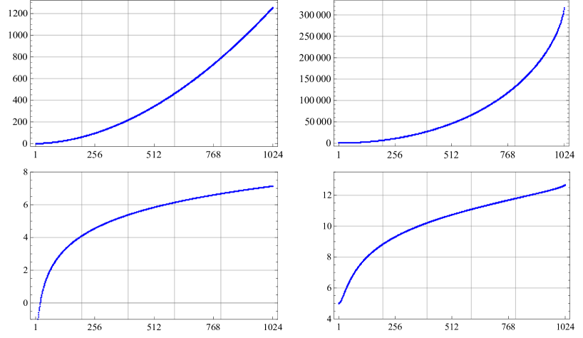
Figure 1: The eigenvalues of $T_{n}(\hat{F}_{n})$ and of $T_{n}^{-1}(\eta)T_{n}(\hat{F}_{n})$ where $\eta(\theta)=\theta^{2}$, for $n=1024$. Regular scale (top) and logarithmic scale (bottom).

5 Conclusions

In this note we have considered a novel type of spectral problem involving Toeplitz structures and arising in the numerical approximation of distributed-order fractional differential equations. The spectral study of the matrices under consideration has been reduced to the study of the matrix

$$T_{n}(g_{0})+h^{h}T_{n}(g_{1})+h^{2h}T_{n}(g_{2})+\cdots+h^{(n-1)h}T_{n}(g_{n-1}),$$

where $h=\frac{1}{n}$, $g_{j}(\theta)=|\theta|^{2-jh}$, and $j=0,\ldots,n-1$. Because the resulting generating function depends on $n$, the standard theory cannot be applied and the analysis has been performed using new ideas. Few selected numerical experiments have been presented and critically discussed. Many open questions remain: we can consider for instance the use of the given spectral information in a context of Krylov preconditioning or multigrid design for large linear systems coming from FDEs with distributed order and the extension of the proposed analysis in a multidimensional context, when the spatial derivatives belong to a $d$-dimensional domain with $d\geqslant 2$. These lines of research will be the subject of future investigations.

References

• [1] Bogoya, M., Böttcher, A., Grudsky, S.M., and Maximenko, E.A. Maximum norm versions of the Szegő and Avram–Parter theorems for Toeplitz matrices. J. Approx. Theory 196 (2015), 79–100.
• [2] Calcagni, G. Towards multifractional calculus. Front. Phys. 6 (2018), 58.
• [3] Caputo, M., and Fabrizio, M. The kernel of the distributed order fractional derivatives with an application to complex materials. Fractal Fract. 1, 1 (2017), 13.
• [4] Chan, R., and Jin, X. An introduction to iterative Toeplitz solvers. Society for Industrial and Applied Mathematics (SIAM), 2007.
• [5] Ding, W., Patnaik, S., Sidhardh, S., and Semperlotti, F. Applications of distributed-order fractional operators: A review. Entropy 23, 1 (2021), 110.
• [6] Donatelli, M., Mazza, M., and Serra-Capizzano, S. Spectral analysis and structure preserving preconditioners for fractional diffusion equations. J. Comput. Phys. 307 (2016), 262–279.
• [7] Donatelli, M., Mazza, M., and Serra-Capizzano, S. Spectral analysis and multigrid methods for finite volume approximations of space-fractional diffusion equations. SIAM J. Sci. Comput. 40, 6 (2018), A4007–A4039.
• [8] Fan, W., and Liu, F. A numerical method for solving the two-dimensional distributed order space-fractional diffusion equation on an irregular convex domain. Appl. Math. Lett. 77 (2018), 114–121.
• [9] Garoni, C., and Serra-Capizzano, S. Generalized Locally Toeplitz sequences: Theory and applications. Vol. I. Springer, Cham, 2017.
• [10] Huang, X., Fang, Z.W., Sun, H.W., and Zhang, C.H. A circulant preconditioner for the Riesz distributed-order space-fractional diffusion equations. Linear Multilinear Algebra 0 (2020), 1–16.
• [11] Korovkin, P.P. Linear Operators and Approximation Theory, (English translation). Hindustan, 1960.
• [12] Li, J., Liu, F., Feng, L., and Turner, I. A novel finite volume method for the Riesz space distributed order diffusion equation. Comput. Math. Appl. 74, 4 (2017), 772–783.
• [13] Mazza, M., Serra-Capizzano, S., and Usman, M. Symbol-based preconditioning for Riesz distributed-order space-fractional diffusion equations. Electr. Trans. Num. Anal. 54 (2021), 499–513.
• [14] Ng, M. Iterative methods for Toeplitz systems. Oxford University Press, 2004.
• [15] Serra-Capizzano, S. On the extreme eigenvalues of Hermitian (block) Toeplitz matrices. Linear Algebra Appl. 270 (1998), 109–129.
• [16] Serra-Capizzano, S. Some theorems on linear positive operators and functionals and their applications. Comput. Math. Appl. 39, 7/8 (2000), 139–167.