Momentum scalar triple product as a measure of chirality in electron ionization dynamics of strongly-driven atoms

Abstract

We formulate a transparent measure that quantifies chirality in single electron ionization triggered in atoms, which are achiral systems. We do so in the context of Ar driven by a new type of optical fields that consists of two non-collinear laser beams giving rise to chirality that varies in space across the focus of the beams. Our computations account for realistic experimental conditions. To define this measure of chirality, we first find the sign of the electron final momentum scalar triple product $\mathrm{{\bf{p}}_{k}\cdot({\bf{p}}_{i}\times{\bf p}_{j})}$ and multiply it with the probability for an electron to ionize with certain values for both $\mathrm{p_{k}}$ and $\mathrm{p_{i}p_{j}}$. Then, we integrate this product over all values of $\mathrm{p_{k}}$ and $\mathrm{p_{i}p_{j}}$. We show this to be a robust measure of chirality in electron ionization triggered by globally chiral electric fields.

Ultrafast phenomena in chiral molecules triggered by intense, infrared laser pulses are at the forefront of laser-matter interactions Cireasa et al. (2015); Beaulieu et al. (2017, 2018); Comby et al. (2018); Rozen et al. (2019). While ultrafast chiral processes can be studied using high harmonic generation (HHG) Cireasa et al. (2015); Ayuso et al. (2019); Baykusheva and Wörner (2018); Neufeld and Cohen (2018); Neufeld et al. (2019); Heinrich et al. (2021), the underlying recollision mechanism entails that a stronger chiral response comes at the expense of a greatly suppressed high harmonic signal Cireasa et al. (2015). Hence, photoelectron spectroscopy is a promising route to a robust signal from molecules driven by intense chiral fields Lux et al. (2012); Lehmann et al. (2013); Boge et al. (2014); Beaulieu et al. (2017, 2018); Rozen et al. (2019). However, the sensitivity of chiral photoelectron spectroscopy also struggles with the fact that laser wavelengths are several orders of magnitude larger than the molecular dimensions, i.e., the chiralities of the optical field and the molecule are incommensurate.

Recently, Ayuso et al. proposed a new type of optical field which is chiral on the atomic scale Ayuso et al. (2019) and thereby holds the potential for unprecedented chiral sensitivity. The chiral field is synthesized by combining two orthogonally polarized two-color laser fields in a non-collinear geometry as illustrated in Fig. 1. The non-collinear geometry creates an intensity and ellipticity grating, and thereby causes the chirality of the laser field to spatially vary across the focus. Thus, it is a fundamental challenge for experiments to decipher the signatures of chirality in the photoelectron spectra from these new laser fields.

Here, we provide a simple prescription on how to analyze experimental photoelectron spectra produced from any type of chiral light. To this end, we perform semi-classical simulations of strong-field ionization, taking into account the focal volume distribution of the degree of light chirality. To develop an understanding of chiral electron ionization we model atomic photoionization, since ground-state atoms have spherical symmetry and are intrinsically achiral systems. Thus, the chiral response of the escaping electron that is imprinted on the ionization spectra in our model arises solely from the dynamics triggered by the electric field of the laser.

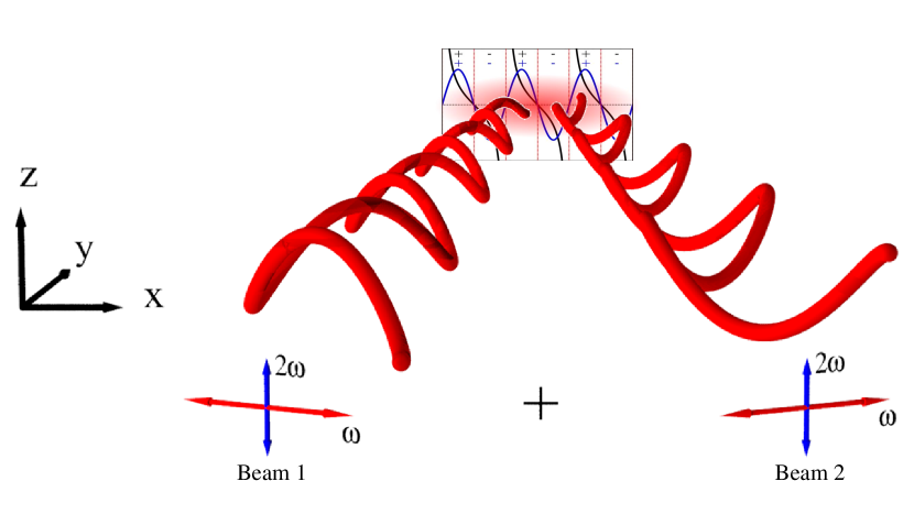
Figure 1: Schematic plot of two non-collinear laser beams, each consisting of $\omega$-$2\omega$ orthogonally polarized linear fields; $\omega$ is polarized on the x-y plane and 2$\omega$ along the z-axis. Both beams propagate towards the atom in the focus region (red-shaded ellipse). The resultant electric field has chirality (square inset) that changes along the x-axis in the focus region.

In order to analyze the resulting photoelectron spectra we identify a transparent measure that quantifies chirality in electron ionization dynamics ensuing from an atom strongly-driven by a chiral electric field. We construct this measure by finding the probability P$(\mathrm{p_{k},p_{i}p_{j}})$ for an electron to ionize with certain values for both $\mathrm{p_{k}}$ and $\mathrm{p_{i}p_{j}}$, with p_i,p_j,p_k being the components of the final electron momentum. Next, we multiply this probability by the sign of the momentum scalar triple product $\mathrm{{\bf{p}}_{k}\cdot({\bf{p}}_{i}\times{\bf p}_{j})}$. Integrating over the whole range of values of $\mathrm{p_{k}}$ and $\mathrm{p_{i}p_{j}}$, we obtain a measure of chirality

$$\begin{split}\mathcal{X}\mathrm{(p_{k},p_{i}p_{j})}&=\\ &\mathrm{\iint sign(\mathrm{{\bf{p}}_{k}\cdot({\bf{p}}_{i}\times{\bf p}_{j})})P(\mathrm{p_{k},p_{i}p_{j}})dp_{i}p_{j}dp_{k}}.\end{split}$$ (1)

We show that $\mathcal{X}$ has an opposite sign for synthetic pulses with opposite chirality, while it is zero for achiral synthetic pulses. This measure of handedness of electron ionization dynamics is a general one and accounts for chiral electron motion triggered by any chiral light.

We demonstrate that $\mathcal{X}$ is a measure of handedness of electron ionization dynamics ensuing from atoms, in the context of Ar driven by two non-collinear laser beams, see Fig. 1. Beams 1, 2 propagate on the x-y plane with wavevectors $\mathbf{k}_{1}$, $\mathbf{k}_{2}$ forming an angle $\alpha$ with the y axis

$$\begin{split}\mathbf{k}_{1}&=\mathrm{k}\sin(\alpha)\hat{\mathbf{x}}+\mathrm{k}\cos(\alpha)\hat{\mathbf{y}}\\ \mathbf{k}_{2}&=-\mathrm{k}\sin(\alpha)\hat{\mathbf{x}}+\mathrm{k}\cos(\alpha)\hat{\mathbf{y}},\end{split}$$ (2)

where $k=\mathrm{2\pi}/\lambda$. The electric field of each beam consists of two orthogonally polarized $\omega$ and $2\omega$ laser fields. The $\omega$ field is polarized along the x-y plane and the $2\omega$ field is polarized along the z-axis. Also, we take the 2$\omega$ field to have small intensity compared to the $\omega$ field.

The resultant electric field is given by Ayuso et al. (2019)

$$\mathbf{E}(\mathbf{r},\mathrm{t})=2\mathrm{E}_{0}\exp\left[-\left(\frac{t}{\tau}\right)^{2}\right]\left(\mathrm{E_{x}}\hat{\mathbf{x}}+\mathrm{E_{y}}\hat{\mathbf{y}}+\mathrm{E_{z}}\hat{\mathbf{x}}\right),$$ (3)

where

$$\begin{split}\mathrm{E_{x/y}}&=\exp\left[-\left(\frac{\rho}{\mathrm{w_{0}}}\right)^{2}\right]\mathrm{f_{x/y}(x)}\cos\left[\mathrm{g(y,t)}\right]\\ \mathrm{E_{z}}&=\exp\left[-\left(\frac{2\rho}{\mathrm{w_{0}}}\right)^{2}\right]\mathrm{f_{z}(x)}\cos\left[\mathrm{h(y,t)}\right],\end{split}$$ (4)

and

$$\begin{split}\mathrm{f_{x}(x)}&=\cos(\alpha)\cos\left[\mathrm{k}\sin(\alpha)x+\frac{\phi_{2}^{\omega}-\phi_{1}^{\omega}}{2}\right]\\ \mathrm{f_{y}(x)}&=\sin(\alpha)\sin\left[\mathrm{k}\sin(\alpha)x+\frac{\phi_{2}^{\omega}-\phi_{1}^{\omega}}{2}\right]\\ \mathrm{f_{z}(x)}&=\mathrm{r_{0}}\cos\left[2\mathrm{k}\sin(\alpha)x+(\phi_{2}^{2\omega}-\phi_{1}^{2\omega})\right]\\ \mathrm{g(y,t)}&=\mathrm{k}\cos(\alpha)\mathrm{y}-\omega\mathrm{t}-\frac{\phi_{2}^{\omega}+\phi_{1}^{\omega}}{2}\\ \mathrm{h(y,t)}&=2\mathrm{k}\cos(\alpha)\mathrm{y}-2\omega\mathrm{t}-(\phi_{2}^{2\omega}+\phi_{1}^{2\omega}).\end{split}$$ (5)

We note that $\tau=25$ fs and $\tau\sqrt{2\ln(2)}$ is the full width at half maximum of the pulse duration in intensity, while $\mathrm{E_{0}}$ is the field strength corresponding to intensity $\mathrm{5\times 10^{13}\;W/cm^{2}}.$ Also, $\rho$ is the radial distance to the propagation axis of each laser beam. Since $\alpha$ is small, $5^{\circ}$, it follows that $\rho\approx\sqrt{\mathrm{x}^{2}+\mathrm{z}^{2}}$. Moreover, $\mathrm{w_{0}=8.49\;\mu m}$ is the beam waist of the $\omega$ laser field, and $\mathrm{r^{2}_{0}}$ is the intensity ratio of 1/100 of the 2$\omega$ versus the $\omega$ field. Finally, the wavelength $\lambda$ of the $\mathrm{\omega}$ field is taken equal to 800 nm.

We treat single electron ionization of driven Ar by employing a three-dimensional (3D) semi-classical model. The only approximation is the initial state. One electron tunnel-ionizes through the field-lowered Coulomb-barrier at time t₀. To compute the tunnel-ionization rate, we employ the quantum mechanical Ammosov-Delone-Krainov (ADK) formula Landau and Lifshitz (2013); Delone and Krainov (1991). We use parabolic coordinates to obtain the exit point of the tunneling electron along the laser-field direction Hu et al. (1997). We set the electron momentum along the laser field equal to zero, while we obtain the transverse momentum by a Gaussian distribution Landau and Lifshitz (2013); Delone and Krainov (1991). The microcanonical distribution is employed to describe the initial state of the initially bound electron Abrines and Percival (1966).

We select the tunnel-ionization time, t₀, randomly in the time interval [-2$\tau$,2$\tau$]. Next, we specify at time $\mathrm{t_{0}}$ the initial conditions for both electrons. Using the three-body Hamiltonian of the two electrons with the nucleus kept fixed, we propagate classically in time the position and momentum of each electron. All Coulomb forces and the interaction of each electron with the electric field in Eq. (3) are fully accounted for with no approximation. To account for the Coulomb singularity, we employ regularized coordinates Kustaanheimo and Stiefel (1965). Here, we use atomic units.

Previous successes of this model include identifying the mechanism underlying the fingerlike structure in the correlated electron momenta for He driven by 800 nm laser fields Emmanouilidou (2008), see also Parker et al. (2006); Staudte et al. (2007); Rudenko et al. (2007). Moreover, we investigated the direct versus the delayed pathway of non-sequential double ionization for He driven by a 400 nm, long duration laser pulse and achieved excellent agreement with fully ab-initio quantum mechanical calculations Emmanouilidou et al. (2011). Also, for low intensities, we have identified a novel mechanism of double ionization, namely, slingshot non-sequential double ionization Katsoulis et al. (2018). In addition, for several observables of non-sequential double ionization, our results have good agreement with experimental results for Ar when driven by near-single-cycle laser pulses at 800 nm Chen et al. (2017).

It was previously shown Ayuso et al. (2019) that the resultant electric field is globally chiral if the relative phases of the $\omega$ and $2\omega$ laser fields in beams 1 and 2, i.e. $\phi_{1}^{2\omega}-\phi_{1}^{\omega}$ and $\phi_{2}^{2\omega}-\phi_{2}^{\omega}$, satisfy the following condition

$$\mathrm{\left(\phi^{2\omega}_{1}-\phi^{\omega}_{1}\right)-\left(\phi^{2\omega}_{2}-\phi^{\omega}_{2}\right)=\dfrac{\pi}{2}+n\pi,\text{with n}\in}\mathbb{Z},$$ (6)

while the resultant electric field is globally achiral when

$$\mathrm{\left(\phi^{2\omega}_{1}-\phi^{\omega}_{1}\right)-\left(\phi^{2\omega}_{2}-\phi^{\omega}_{2}\right)=n\pi,\text{with n}\in}\mathbb{Z}.$$ (7)

To illustrate that $\mathcal{X}$ is a measure of chirality in electron ionization of driven atoms, we perform six independent studies. Each study corresponds to Ar being driven by one of six different resultant electric fields corresponding to six different synthetic pulses. For simplicity, we refer to the resultant electric field of the synthetic pulse as electric field. Each of the six synthetic pulses (cases 1-6) corresponds to a different combination of $\phi_{1}^{2\omega}-\phi_{1}^{\omega}$ and $\phi_{2}^{2\omega}-\phi_{2}^{\omega}$ for beams 1 and 2, respectively, see Fig. 2(a). Using the conditions in Eq. (6) and Eq. (7), we select four globally chiral electric fields, cases 1,2,4,5, and two globally achiral fields, cases 3, 6, see Fig. 2. In Fig. 2(b), we show that the electric fields which are globally chiral maintain the same handedness along the x-axis in the focus region. That is, E_y(x)/E_x(x) and E_z(x) change sign at the same points in space x. As a result, electric fields 1 and 4 have the same chirality (+) in Fig. 2(b) and electric fields 2 and 5 have the same chirality (-) in Fig. 2(b). It follows that the pairs of electric fields (1,2) and (4,5) have opposite chirality. Also, when E_y(x)/E_x(x) and E_z(x) change sign at different points in space x as defined by Eq. (7), the chirality of the electric field flips sign along the x-axis in the focus region. Hence, the electric field has no overall chirality. This is the case for the globally achiral fields 3 and 6 shown in Fig. 2(b).

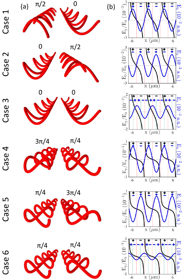
Figure 2: (a) Schematic plots of six combinations of two non-collinear beams; (b) change of sign of E_y(x)/E_x(x) (black) and E_z(x) (blue) along the x-axis in the focus region, at y=z=0, t=T/50. Cases 1,2 correspond to globally chiral electric fields with opposite handedness, the same holds for cases 4 and 5. Cases 3 and 6 correspond to globally achiral electric fields. For each case, above beams 1 and 2, we denote $\phi_{1}^{2\omega}-\phi_{1}^{\omega}$ and $\phi_{2}^{2\omega}-\phi_{2}^{\omega}$, respectively.

Next, we describe how we obtain the electron ionization spectra of Ar for each of the six synthetic pulses (cases 1-6). For simplicity, for each case, we set $\phi_{2}^{\omega}=0$. Since only the differences $\phi_{1}^{2\omega}-\phi_{1}^{\omega}$ and $\phi_{2}^{2\omega}-\phi_{2}^{\omega}$ are important, there is no loss of generality. Moreover, for each of the six synthetic pulses, to simulate realistic experimental conditions, we select 101 equally spaced values of the phase $\mathrm{\phi_{1}^{\omega}}$ in the interval [0,2$\pi$). This allows us to account for the nucleus being at different positions along the x-axis in the focus region. Next, for each of the 101 values of $\mathrm{\phi_{1}^{\omega}}$, we register the single ionisation events and obtain the electron ionization spectra. Then, we average over all $\mathrm{\phi_{1}^{\omega}}$ values and obtain the electron spectra $\mathrm{P^{m}}(\mathrm{p_{x}},\mathrm{p_{y}p_{z}})$, $\mathrm{P^{m}}(\mathrm{p_{y}},\mathrm{p_{z}p_{x}})$ and $\mathrm{P^{m}}(\mathrm{p_{z}},\mathrm{p_{x}p_{y}})$. We normalize each one of these spectra to one. The m index corresponds to the m electric field, i.e. to case m and ranges from 1-6. For each synthetic pulse 1-6, the electron ionization spectra are obtained using at least 10⁷ singly ionizing trajectories.

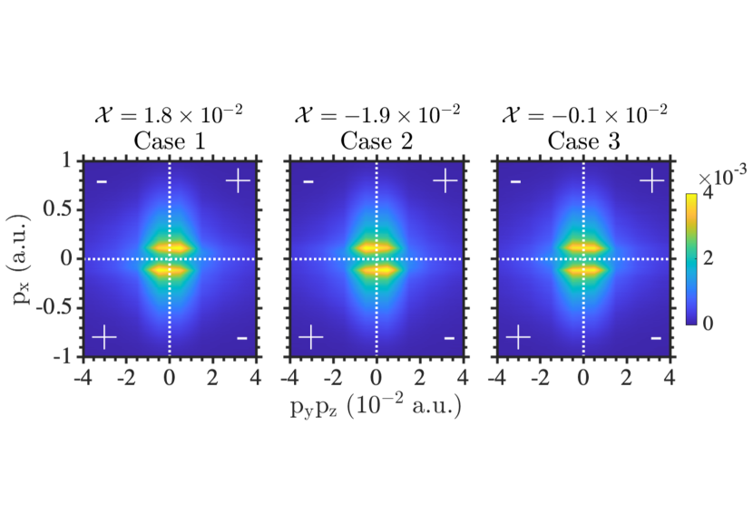
Figure 3: Probability distribution $\mathrm{P^{m}}(\mathrm{p_{x}},\mathrm{p_{y}p_{z}})$ for the electron to ionize with momenta $\mathrm{p_{x}}$ and $\mathrm{p_{y}p_{z}}$, with m=1,2,3 for electric fields 1,2,3, respectively. The sign in each quadrant corresponds to the sign of $\mathrm{{\bf{p}}_{x}\cdot({\bf{p}}_{y}\times{\bf p}_{z})}$ in this quadrant.

In Fig. 3, we plot the probability distribution $\mathrm{P^{m}}(\mathrm{p_{x}},\mathrm{p_{y}p_{z}})$ for an electron to singly ionize with momenta p_x and p$\mathrm{{}_{y}p_{z}}$ for the globally chiral 1, 2 and globally achiral 3 electric fields. In each quadrant we assign the sign resulting from the scalar triple product $\mathrm{{\bf{p}}_{x}\cdot({\bf{p}}_{y}\times{\bf p}_{z})}$. Next, using Eq. (1), we compute the measure of chirality in electron ionization $\mathcal{X}(\mathrm{p_{x}},\mathrm{p_{y}p_{z}})$. We find it to be equal to $1.8\times 10^{-2},-1.9\times 10^{-2},-0.1\times 10^{-2}$ for electric fields 1,2,3, respectively. Indeed, a close inspection of Fig. 3 for case 1 reveals that the probability distribution of the electron momenta p_x and p$\mathrm{{}_{y}p_{z}}$ has larger values at the first and third quadrants, where $\mathrm{{\bf{p}}_{x}\cdot({\bf{p}}_{y}\times{\bf p}_{z})}$ has a + sign. It follows that $\mathcal{X}$ has a positive value when Ar is driven by synthetic pulse 1. In contrast, in Fig. 3 for case 2 the probability distribution of the electron momenta p_x and p$\mathrm{{}_{y}p_{z}}$ has larger values at the second and fourth quadrants, where $\mathrm{{\bf{p}}_{x}\cdot({\bf{p}}_{y}\times{\bf p}_{z})}$ has a - sign. Hence, $\mathcal{X}$ has a negative value for case 2. The opposite signs of $\mathcal{X}$ when Ar is driven by electric fields 1 and 2 are consistent with the opposite chirality of these fields. Moreover, $|\mathcal{X}|$ is roughly the same for cases 1 and 2. The small offset is due to the statistical error introduced in our computations from the number of single ionization events considered. This is also supported by $\mathcal{X}$ being equal to $-0.1\times 10^{-2}$, instead of zero, when Ar is driven by the achiral field 3.

Very interestingly, we find that all three measures of chirality $\mathcal{X}\mathrm{(p_{x},p_{y}p_{z})}$, $\mathcal{X}\mathrm{(p_{y},p_{z}p_{x})}$ and $\mathcal{X}\mathrm{(p_{z},p_{x}p_{y})}$ have the same values for electric field 1, 2 and 3. That is, all three measures are equal to $1.8\times 10^{-2}$ for electric field 1, equal to -$1.9\times 10^{-2}$ for field 2 and equal to -$0.1\times 10^{-2}$ for field 3, see Table 1. The same is true for all three measures of chirality $\mathcal{X}$ when Ar is driven by synthetic pulses 4,5,6. Indeed, all three $\mathcal{X}$ are equal to 1.$\times 10^{-2}$ for electric field 4, equal to $-1.1\times 10^{-2}$ for electric field 5 and equal to -$0.1\times 10^{-2}$ for electric field 6, see Table II. The above further corroborate that $\mathcal{X}$ is a robust measure of chirality in electron ionization triggered by a chiral field, yielding the same value for any of the three combinations of the components of the final electron momentum.

Table 1: Measure of chirality $\mathcal{X}$ in electron ionization for globally chiral electric fields 1,2,4,5, and globally achiral fields 3,6. $\mathcal{X}$ is computed for each of the three $\mathrm{P^{m}}(\mathrm{p_{x}},\mathrm{p_{y}p_{z}})$, $\mathrm{P^{m}}(\mathrm{p_{y}},\mathrm{p_{z}p_{x}})$ and $\mathrm{P^{m}}(\mathrm{p_{z}},\mathrm{p_{x}p_{y}})$, and m ranges from 1-6. The values are expressed in $10^{-2}.$

Case	$\mathcal{X}\mathrm{\left(p_{x},p_{y}p_{z}\right)}$	$\mathcal{X}\mathrm{\left(p_{y},p_{z}p_{x}\right)}$	$\mathcal{X}\mathrm{\left(p_{z},p_{x}p_{y}\right)}$
1	1.8	1.8	1.8
2	-1.9	-1.9	-1.9
3	-0.1	-0.1	-0.1
4	1.0	1.0	1.0
5	-1.1	-1.1	-1.1
6	-0.1	-0.1	-0.1

Next, we outline a yet more transparent way to demonstrate chirality in electron ionization. Namely, we plot $\mathcal{P}^{\mathrm{m,n}}(\mathrm{p_{k},p_{i}p_{j}})$ defined as the difference of the normalized probability distributions in the following way

$$\mathcal{P}^{\mathrm{m,n}}(\mathrm{p_{k},p_{i}p_{j}})=\mathrm{P^{m}(p_{k},\mathrm{p_{i}p_{j}})}-\mathrm{P^{n}(\mathrm{p_{k},p_{i}p_{j}})},$$ (8)

The corresponding measure of chirality is given by

$$\begin{split}&\mathcal{X}d\mathrm{(p_{k},p_{i}p_{j})}=\\ &\mathrm{\iint sign(\mathrm{{\bf{p}}_{k}\cdot({\bf{p}}_{i}\times{\bf p}_{j})})\mathcal{P}^{\mathrm{m,n}}(\mathrm{p_{k},p_{i}p_{j}})dp_{i}p_{j}dp_{k}}.\end{split}$$ (9)

In Figs. 4(a1)-4(a3), we plot the probability distribution $\mathcal{P}^{\mathrm{m,n}}(\mathrm{p_{x}},\mathrm{p_{y}p_{z}})$ for the pair of opposite chirality electric fields (1,2), i.e. Case1-Case 2 (Fig. 4(a1)), and for the pairs of chiral-achiral electric fields (1,3) and (2,3), i.e. Case 1-Case 3 (Fig. 4(a2)) and Case 2-Case 3 ( Fig. 4(a3)). In each quadrant, we assign the sign resulting from the scalar triple product $\mathrm{{\bf{p}}_{x}\cdot({\bf{p}}_{y}\times{\bf p}_{z})}$. The yellow (blue) color denotes positive (negative) values of $\mathcal{P}^{\mathrm{m,n}}(\mathrm{p_{x}},\mathrm{p_{y}p_{z}})$, corresponding to the electron being more (less) probable to ionize with momenta p_x and p$\mathrm{{}_{y}p_{z}}$ due to pulse m rather than pulse n. Next, in each quadrant, we multiply the $\pm$ sign (yellow/blue), resulting from the distribution, with the $\pm$ sign of $\mathrm{{\bf{p}}_{x}\cdot({\bf{p}}_{y}\times{\bf p}_{z})}$ and then sum up. It easily follows that the measure of chirality $\mathcal{X}d\mathrm{\left(p_{x},p_{y}p_{z}\right)}$ is larger and positive ($3.7\times 10^{-2}$) for the pair of opposite chirality fields (1,2), see (Fig. 4(a1)). Also, $\mathcal{X}d$ is positive ($1.9\times 10^{-2}$) for the pair of electric fields (1,3) and negative ($-1.8\times 10^{-2}$) for the pair (2,3), with $1.9\times 10^{-2}-1.8\times 10^{-2}$ being roughly zero, since pulses 1 and 2 have opposite chirality. As for chirality measures $\mathcal{X}$, we find that all three measures of chirality $\mathcal{X}d\mathrm{(p_{x},p_{y}p_{z})}$, $\mathcal{X}d\mathrm{(p_{y},p_{z}p_{x})}$ and $\mathcal{X}d\mathrm{(p_{z},p_{x}p_{y})}$ have the same value for each of the fields 1,2,3, see Table 2.

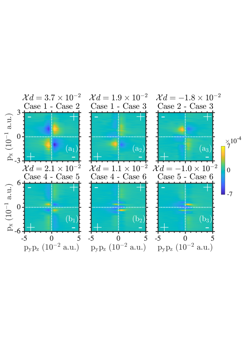
Figure 4: Probability distribution $\mathcal{P}^{\mathrm{m,n}}(\mathrm{p_{x},p_{y}p_{z}})$. The m,n indexes are 1,2 for Case 1-Case 2, 1,3 for Case 1-Case 3 and 2,3 for Case 2-Case 3. The sign in each quadrant corresponds to the sign of $\mathrm{{\bf{p}}_{x}\cdot({\bf{p}}_{y}\times{\bf p}_{z})}$ in this quadrant.

Table 2: Measure of chirality $\mathcal{X}d$ for globally chiral electric fields 1,2,4,5 and globally achiral fields 3,6. $\mathcal{X}d$ is computed for each of the three probability distributions $\mathcal{P}^{\mathrm{m,n}}(\mathrm{p_{x}},\mathrm{p_{y}p_{z}})$, $\mathcal{P}^{\mathrm{m,n}}(\mathrm{p_{y}},\mathrm{p_{z}p_{x}})$ and $\mathcal{P}^{\mathrm{m,n}}(\mathrm{p_{z}},\mathrm{p_{x}p_{y}})$. The values are expressed in $10^{-2}$.

m	n	$\mathcal{X}d\mathrm{\left(p_{x},p_{y}p_{z}\right)}$	$\mathcal{X}d\mathrm{\left(p_{y},p_{z}p_{x}\right)}$	$\mathcal{X}d\mathrm{\left(p_{z},p_{x}p_{y}\right)}$
1	2	3.7	3.7	3.7
1	3	1.9	1.9	1.9
2	3	-1.8	-1.8	-1.8
4	5	2.1	2.1	2.1
4	6	1.1	1.1	1.1
5	6	-1.0	-1.0	-1.0

A similar analysis holds for the measures of chirality in electron ionization when Ar is driven by the globally chiral electric fields 4,5 and the globally achiral field 6. Indeed, in Figs. 4(b1)-4(b3), we plot the probability distribution $\mathcal{P}^{\mathrm{m,n}}(\mathrm{p_{x}},\mathrm{p_{y}p_{z}})$ corresponding to the pair of opposite chirality electric fields (4,5), Case 4-Case 5, and to the pairs of chiral-achiral pulses (4,6), Case 4-Case 6, and (5,6), Case 5-Case 6. As for our results for electric fields 1,2,3, we find that $\mathcal{X}d\mathrm{\left(p_{x},p_{y}p_{z}\right)}$ for the pair of opposite chirality fields (4,5) has the largest value of $2.1\times 10^{-2}$. Also, as expected, for the pairs (4,6) and (5,6), we find that $\mathcal{X}d$ has roughly opposite values, $1.1\times 10^{-2}$ and $-1.0\times 10^{-2}$. The exact same results hold for $\mathcal{X}d$ obtained for the other two combinations of momentum components for fields 4,5,6, see Table 2.

Summarizing, we identify a transparent and simple measure of chirality in electron ionization triggered in atoms (Ar) by synthetic pulses. These pulses can create electric fields which are globally chiral or achiral along the focus region. Our computations account for realistic experimental conditions. We define this measure by multiplying the sign of the final electron momentum scalar triple product $\mathrm{{\bf{p}}_{k}\cdot({\bf{p}}_{i}\times{\bf p}_{j})}$ with the probability for an electron to ionize with certain values for both p_k and p_ip_j. Finally, we integrate over all values of p_k and p_ip_j. Three such measures can be defined, corresponding to the three combinations of p_k and p_ip_j. We find that all three measures of chirality have the same value for a given electric field. This robust measure of chirality has opposite values when the electron dynamics is triggered by fields with opposite chirality and is zero for a globally achiral field. We expect that this measure of chirality in electron ionization of atoms applies to any chiral field.