Multi-level computation of the hadronic vacuum polarization contribution to $(g_{\mu}-2)$

Abstract

The first results from the Fermilab E989 experiment have confirmed the long-standing tension between the experimental determination of the muon anomalous magnetic moment $a_{\mu}=(g_{\mu}-2)/2$ and its SM determination using the dispersive approach. In order to match the expected final precision from E989, the current uncertainty on ab initio determinations using lattice QCD must be decreased by a factor 5-15, a goal which is hampered by the signal-to-noise ratio problem of the electromagnetic current correlator. Multi-level Monte Carlo integration with fermions is a method which reduces the variance of correlators exponentially in the distance of the fields. Here we demonstrate that the variance reduction in a realistic two-level simulation with a pion mass of 270 MeV, linear size of 3 fm and lattice spacing around 0.065 fm is sufficient to compute the tail of the current correlator with the statistical accuracy required for the hadronic vacuum polarization contribution to $a_{\mu}$. An efficient estimator is also employed for computing the disconnected contribution.

CERN–TH–2021–203

1 Introduction

The muon anomalous magnetic moment, $a_{\mu}$, has been measured about 15 years ago by the E821 experiment at BNL with the impressive precision of $0.54$ parts per million (ppm) [1]. That measurement has been recently confirmed by the first data from the on-going E989 experiment at FNAL and the combination of the two results have provided the currently best experimental estimate $a_{\mu}=11659206.1(4.1)\times 10^{-10}$ [2]. At the end of its operation period, the E989 experiment is expected to attain the astonishing precision of $0.14$ ppm.

In the Standard Model (SM) the value of $a_{\mu}$ results from the combination of various effects that have been computed theoretically: there are contributions from Quantum Electrodynamics and from the Weak Interactions that have been calculated perturbatively up to five loops and two loops, respectively, as well as from the Strong Interactions coming from the Hadronic leading-order Vacuum Polarization (HVP) and the Hadronic Light-by-Light scattering (HLbL) [4]. The final theoretical uncertainty is currently dominated by the hadronic part and, thus, it represents the main target to improve the accuracy of the theoretical prediction. Since the purely theoretical computations are not sufficiently precise at the moment the hadronic contributions have been extracted (by assuming the SM) from experimental data via dispersive integrals (HVP & HLbL) and low-energy effective models supplemented with the operator product expansion (HLbL). The overall theoretical expectation leads to $a_{\mu}=11659181.0(4.3)\times 10^{-10}$ (0.37 ppm) [4], which deviates by 4.2 standard deviations from the experimental value. That difference has by now been persisting for more than a decade and it may be a hint for New Physics.

Although state-of-the-art lattice Quantum Chromodynamics (QCD) determinations of the HVP are steadily improving their accuracy and they are becoming competitive, the overall error on $a_{\mu}$ is still 5-15 times larger than the anticipated uncertainty from E989. In fact, currently quoted uncertainties range between $0.8\%$ to roughly $2\%$, see Ref. [4] and references therein. The main difficulty in matching the level of precision of the experimental result lays in the large statistical error of the Monte Carlo evaluation of the required correlation functions [4]. In a recent investigation [5], we have proposed a solution to that problem based on a multi-level Monte Carlo integration algorithm in the presence of fermions [6, 7]. The novel computational paradigm of this method with respect to the standard approach allows to reduce exponentially the variance of a correlation function with the temporal distance of the fields. As a first application, we have performed a feasibility study on the HVP, but the strategy is general and it can be applied to the HLbL, to the isospin-breaking and to the electromagnetic contributions as well.

2 The problem of the signal-to-noise ratio

A useful way of writing the HVP suitable for numerical calculations is given by

$$a_{\mu}^{\rm HVP}=\left(\frac{\alpha}{\pi}\right)^{2}\int_{0}^{\infty}dx_{0}\,K(x_{0},m_{\mu})\,G(x_{0})\;,$$ (1)

where $\alpha$ is the electromagnetic coupling constant, $K(x_{0},m_{\mu})$ is a known function increasing quadratically at large $x_{0}$, $m_{\mu}$ is the muon mass, and $G(x_{0})$ is the zero-momentum correlation function

$$G(x_{0})=\int d^{3}{\bf x}\,\langle J_{k}^{em}(x)J_{k}^{em}(0)\rangle$$ (2)

of two electromagnetic currents $J_{k}^{em}=i\sum_{i=1}^{N_{f}}q_{i}\bar{\psi}_{i}\gamma_{k}\psi_{i}$; for unexplained notation we refer to Ref. [5]. In this study we consider $N_{f}=3$, namely the 3 lighter quarks of QCD with the first 2 degenerate in mass, and the correlation function is given by the sum of the following contributions

$$G(x_{0})=G^{\rm conn}_{u,d}(x_{0})+G^{\rm conn}_{s}(x_{0})+G^{\rm disc}_{u,d,s}(x_{0})\;.$$ (3)

The first and the last terms are the light-connected Wick contraction, $G^{\rm conn}_{u,d}(x_{0})$, and the disconnected one, $G^{\rm disc}_{u,d,s}(x_{0})$: they represent the most problematic and numerically challenging contributions to evaluate. In fact, in standard Monte Carlo computations, the relative error of the former at large time distances $|x_{0}|$ goes as

$$\frac{\sigma^{2}_{{}_{G^{\rm conn}_{\rm u,d}}}(x_{0})}{[G^{{\rm conn}}_{\rm u,d}(x_{0})]^{2}}\propto\frac{1}{n_{0}}\;e^{2\,(M_{\rho}-M_{\pi})|x_{0}|}\;,$$ (4)

where $M_{\rho}$ is the lightest asymptotic state in the iso-triplet vector channel, and $n_{0}$ is the number of independent field configurations. This shows that the exponential loss of the signal accuracy with the distance $|x_{0}|$ has to be compensated by a corresponding exponential increase of the statistics $n_{0}$ and, thus, of the computational effort. The situation for the disconnected contribution, $G^{\rm disc}_{u,d,s}(x_{0})$, is even worse because the exponential degradation of the signal is faster since the variance is constant in time. This exponential increase of the relative error is the bottleneck that is currently preventing to obtain a per-mille statistical precision on the HVP by Monte Carlo simulations of QCD on the lattice.

3 The fermionic multi-level algorithm

In the last few years an important conceptual, algorithmic and technical progress has been pursued and it is now possible to carry out multi-level Monte Carlo simulations also in the presence of fermions [6, 7]. In this approach, the lattice is initially decomposed into two overlapping domains $\Omega_{0}$ and $\Omega_{2}$ – see e.g. Fig. 1 – which share a common region $\Lambda_{1}$: it is chosen so that the minimum distance between the points belonging to the inner domains $\Lambda_{0}$ and $\Lambda_{2}$ remains finite and positive in the continuum limit. Then, following the above decomposition, the determinant of the Hermitean massive Wilson-Dirac operator $Q=\gamma_{5}D$ is rewritten as the product of determinants of several operators

$$\det\,Q=\frac{\det\,\left(1-w\right)}{\det\,Q_{\Lambda_{1}}\det\,Q^{-1}_{\Omega_{0}}\det\,Q^{-1}_{\Omega_{2}}}\;,$$ (5)

where $Q_{\Lambda_{1}}$, $Q_{\Omega_{0}}$, and $Q_{\Omega_{2}}$ indicate the very same operator restricted to the domains specified by the subscript. They are obtained from $Q$ by imposing Dirichlet boundary conditions on the external boundaries of each domain. The matrix $w$ is built out of $Q_{\Omega_{0}}$, $Q_{\Omega_{2}}$ and the hopping terms of the operator $Q$ across the boundaries in between the inner domains $\Lambda_{0}$ and $\Lambda_{2}$ and the common region $\Lambda_{1}$ [7]. In the denominator the dependence on the gauge field is already factorized because $\det Q_{\Lambda_{1}}$, $\det\,Q^{-1}_{\Omega_{0}}$ and $\det\,Q^{-1}_{\Omega_{2}}$ depend only on the gauge field in $\Lambda_{1}$, $\Omega_{0}$ and $\Omega_{2}$ respectively.

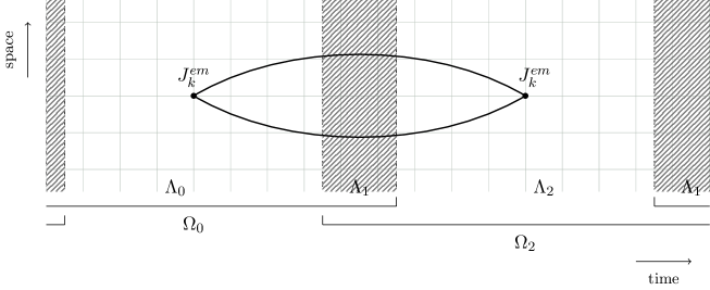
Figure 1: Decomposition of the lattice in domains as described in the text; periodic and anti-periodic boundary conditions in the time direction are enforced for gluons and fermions, respectively.

Finally, we re-express the numerator in Eq. (5) as

$$\det\,\left(1-w\right)=\frac{\det\,[1-R_{N+1}(1-w)]}{C\prod_{k=1}^{N/2}{\det}\big{[}(u_{k}-w)^{\dagger}(u_{k}-w)\big{]}}\,,$$ (6)

where $u_{k}$ and $u^{*}_{k}$ stand for the $N$ roots of a polynomial approximant for $(1-w)^{-1}$, the numerator is the remainder, and $C$ is an irrelevant constant. The purpose of this rewriting is that the denominator in Eq. (6) can be represented by an integral over a set of $N/2$ multi-boson fields [5, 6, 7] having an action with a factorized dependence on the gauge field in $\Lambda_{0}$ and $\Lambda_{2}$ inherited from $w$. By a proper choice of the polynomial approximation, the remainder in the numerator of Eq. (6) fluctuates mildly with the gauge field and it can be included in the observable as a reweighting factor.

In Fig. 1 we show a convenient decomposition of the lattice: the two regions $\Lambda_{0}$ and $\Lambda_{2}$ have the shape of thick time-slices while $\Lambda_{1}$ includes the rest of the lattice and it has the shape of thinner time-slices that keep the first two regions apart. Taking into account the short-distance suppression of the quark propagator, a thickness of $0.5$ fm or so for the slices forming $\Lambda_{1}$ is good enough to make $\Lambda_{0}$ and $\Lambda_{2}$ weakly correlated, furthermore it is not expected to vary significantly with the quark mass. This is the domain decomposition that we use for the numerical computations presented here.

A two-level scheme is used in the Monte Carlo simulation. As a first step, $n_{0}$ well-decorrelated, level-$0$ gauge field configurations are generated by updating the field over the whole lattice: they represent the starting point of the update at level-$1$. This second step is accomplished as follows: in every level-$0$ configuration the gauge field in the overlapping region $\Lambda_{1}$ is kept fixed and $n_{1}$ level-$1$ configurations are generated by updating the field in $\Lambda_{0}$ and in $\Lambda_{2}$ independently thanks to the factorization of the action. The resulting gauge fields are then combined in all possible ways obtaining effectively $n_{0}\cdot n_{1}^{2}$ configurations at the cost of generating $n_{0}\cdot n_{1}$ gauge fields over the entire lattice. Past experience on two-level integration suggests that, with two independently updated regions, the variance decreases proportionally to $1/n_{1}^{2}$ until the standard deviation of the estimator is comparable with the signal, i.e. until the level-$1$ integration has solved the signal-to-noise problem. From Eq. (4) we thus conclude that, as expected, the variance reduction due to level-$1$ integration grows exponentially with the time-distance of the currents in Eq. (2).

4 The numerical study

In this section we present the results of a study on the efficiency of the two-level Monte Carlo algorithm. We have performed numerical simulations of QCD with two dynamical flavours supplemented by a valence strange quark on a lattice of size $96\times 48^{3}$ with a spacing of $\;a=0.065$ fm, and with a pion mass of $270$ MeV. The lattice has been decomposed such that the domains $\Lambda_{0}$ and $\Lambda_{2}$ are made of $40$ consecutive time-slices separated by two regions of $8$ time-slices each which form the region $\Lambda_{1}$. We use the standard pseudofermion representation for the determinants at the denominator of Eq. (5) while the number of multi-bosons is fixed to $N=12$. We consider the same action and the same set of auxiliary fields both at level-$0$ and at level-$1$. The reweighting factor is estimated stochastically with 2 random sources which are sufficient for making its contribution to the statistical error negligible. At level-0 we have generated $n_{0}=25$ configurations and then, for each of them, $n_{1}=10$ configurations in $\Lambda_{0}$ and in $\Lambda_{2}$ have been produced. In Refs. [5, 6, 7] one can find further details on the algorithm and its implementation.

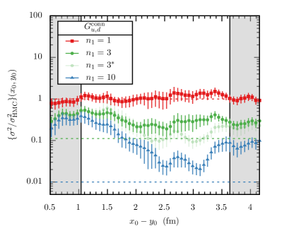
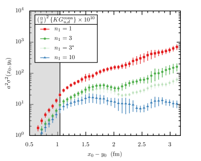
Figure 2: Left panel: dependence of the variance of the light-connected contraction on the difference between the time-coordinates of the currents for $n_{1}=1,3,10$. Data are normalized to the analogous ones computed on CLS configurations generated by one-level HMC. Dashed lines represent the maximum reduction, $1/n^{2}_{1}$, that can be obtained by the two-level integration with decorrelated level-$1$ configurations. Grey bands indicate the thick time-slices where the gauge field is kept fixed during level-$1$ updates. Right panel: variance of the light-connected contribution to the integrand in Eq. (1).

We have carried out a dedicated calculation of the correlation functions in order to assess the reduction of the variance due only to two-level averaging. The light-connected contraction has been calculated by averaging over $216$ local sources located on the time-slice $y_{0}/a=32$ of $\Lambda_{0}$ – corresponding to a distance of $8$ lattice spacings from its right boundary – and by summing over the sink space-position. For what concerns the disconnected contraction, each single-propagator trace has been averaged over 768 Gaussian random sources so to have a negligible random-noise contribution to the variance [5, 8].

In the left panel of Fig. 2 we show the variance of the light-connected contribution as a function of the distance from the source: for sake of readability only the time-slices belonging to $\Omega_{2}$ are displayed, i.e. those relevant for studying the effect of two-level integration given the source position. Data are normalized to the variance obtained with the same number of sources on CLS configurations which were generated with a conventional one-level HMC. The data clearly provide evidence of the exponential reduction of the variance with the distance from the source with the maximum gain reached from $2.5$ fm onward for $n_{1}=10$. We observe a mild reduction with respect to the ideal scaling $n_{1}^{2}$ by a factor between $2$ and $3$ either for $n_{1}=3$ or $10$ (dashed lines): this could be related to a residual correlation among level-$1$ configurations. The power of the two-level integration is also shown in the right panel of Fig. 2, where the variance of the light-connected contribution to the integrand in Eq. (1) is plotted as a function of the time-distance of the currents. The sharp rising of the variance computed by one-level Monte Carlo ($n_{1}=1$, red squares) is automatically flattened out by the two-level multi-boson domain-decomposed HMC ($n_{1}=10$, blue triangles) without the need for modeling the long-distance behaviour of $G^{\rm conn}_{u,d}(x_{0})$.

Finally, we compute the dependence of the integral in Eq. (1) on the upper extrema of integration $x_{0}^{\rm max}$: for $n_{1}=1$, the integral reads $446(26)$ and $424(38)$ for $x_{0}^{\rm max}=2.5$ and $3.0$ fm respectively, while for $n_{1}=10$ the corresponding values are $467.0(8.4)$ and $473.4(8.6)$. It is interesting to note that with the one-level integration the errors on the contributions to the integral from $0$ to $2.5$ fm and from $2.5$ to the maximum value of $3.0$ fm are comparable, while with the two-level HMC the contribution to the variance from the long distance part becomes negligible. Similar remarks hold for the much smaller disconnected contribution.

5 Results and discussion

On the l.h.s. of Fig. 3 our best result for the light-connected contribution to the integrand in Eq. (1) are plotted with red squares. These results are obtained by a weighted average of the above discussed correlation function computed on $32$ point sources per time-slice on $7$ time-slices at $y_{0}/a=\{8,16,24,56,64,72,80\}$ and on $216$ sources at $y_{0}/a=32$. The statistical accuracy is good up to the maximum distance of $3$ fm or so. The contribution coming from the connected contraction of the strange quark, $G^{\rm conn}_{s}(x_{0})$, is much less noisy, and it is accurately determined by averaging over $16$ point sources at $y_{0}/a=32$. It is at most one order of magnitude smaller than the light-connected one and the impact of the statistical error on the final accuracy is negligible. The data are shown using blue circles in the left plot of Fig. 3. The disconnected contribution has been computed as discussed in the previous section and the numerical results are shown in the left plot of Fig. 3 using green triangles. We observe a negative peak at about $1.5$ fm, and a good statistical signal is obtained up to $2.0$ fm or so. Its absolute value is more than two orders of magnitude smaller than the light-connected contribution over the entire range explored.

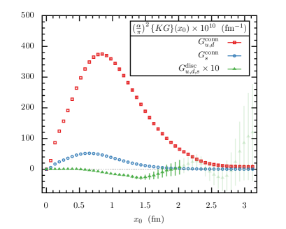
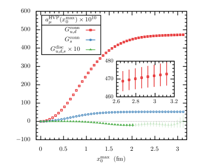
Figure 3: Best results for contribution of the light-connected (red squares), strange-connected (blue circles) and disconnected (green triangles) contractions to the integrand in Eq. (1) (left panel) and to $a_{\mu}^{\rm HVP}$ (right panel) as a function of the time coordinate $x_{0}^{\rm max}$.

The best values of the light-connected (red squares), of the strange-connected (blue circles), and of the disconnected (green triangles) contributions to $a_{\mu}^{\rm HVP}\cdot 10^{10}$ are shown in the right plot of Fig. 3 as a function of the upper extrema of integration $x_{0}^{\rm max}$ in Eq. (1). The light-connected part starts to flatten out at $x_{0}^{\rm max}\sim 2.5$ fm and, at the conservative distance of $x_{0}^{\rm max}=3.0$ fm, its value is $471.8(6.2)$. At the same distance the value of the strange-connected contribution is $52.55(21)$ with a negligible error with respect to the light-connected one. For what concerns the disconnected contribution, it starts to flatten out at about $x_{0}^{\rm max}\sim 2.0$ fm, where its value is $-1.98(84)$. For $x_{0}^{\rm max}=3.0$ fm, its statistical uncertainty is $2.1$ which is still 3 times smaller with respect to the light-connected one. Although the disconnected contribution is very small it must be taken into account to attain the target per-mille precision on the HVP; the combined usage of split-even estimators [8] and two-level integration solves the problem of its computation that has represented a numerical challenge for quite some time. By combining the connected contributions at $x_{0}^{\rm max}=3.0$ fm with the disconnected part at $x_{0}^{\rm max}=2.0$ fm, the best final estimate is $a_{\mu}^{\rm HVP}=522.4(6.2)\cdot 10^{-10}$.

In this investigation we demonstrate the effectiveness of the fermionic multi-level algorithm by achieving a 1% statistical precision with just $n_{0}\cdot n_{1}=250$ configurations on a realistic lattice. This shows that, for the light-quark mass considered here, a per-mille statistical precision on $a_{\mu}^{\rm HVP}$ is reachable by increasing $n_{0}$ and $n_{1}$ by a factor of about $4$–$6$ and $2$–$4$ respectively. For lighter up and down quarks, the gain due to the multi-level integration is expected to increase exponentially in the quark mass, hence improving even more dramatically the scaling of the simulation cost with respect to a standard one-level Monte Carlo. In conclusion, the change of computational paradigm discussed here overcomes the main barrier that prevents to reach a per-mille precision on $a_{\mu}^{\rm HVP}$ on computers available today.

References

- [1] G. W. Bennett, et al., Phys. Rev. D73 (2006) 072003, arXiv:hep-ex/0602035.
- [2] B. Abi et al. [Muon g-2], Phys. Rev. Lett. 126 (2021) no.14, 141801, arXiv:2104.03281.
- [3] J. Grange, et al., arXiv:1501.06858.
- [4] T. Aoyama, et al., Phys. Rept. 887 (2020), 1-166, arXiv:2006.04822.
- [5] M. Dalla Brida, L. Giusti, T. Harris and M. Pepe, Phys. Lett. B 816 (2021), 136191, arXiv:2007.02973.
- [6] M. Cè, L. Giusti, S. Schaefer, Phys. Rev. D93 (9) (2016) 094507, arXiv:1601.04587.
- [7] M. Cè, L. Giusti, S. Schaefer, Phys. Rev. D95 (3) (2017) 034503, arXiv:1609.02419.
- [8] L. Giusti, et al., Eur. Phys. J. C79 (7) (2019) 586, arXiv:1903.10447.