Explainable Deep Learning in Healthcare: A Methodological Survey from an Attribution View [Advanced Review]
Abstract
The increasing availability of large collections of electronic health record (EHR) data and unprecedented technical advances in deep learning (DL) have sparked a surge of research interest in developing DL based clinical decision support systems for diagnosis, prognosis, and treatment. Despite the recognition of the value of deep learning in healthcare, impediments to further adoption in real healthcare settings remain due to the black-box nature of DL. Therefore, there is an emerging need for interpretable DL, which allows end users to evaluate the model decision making to know whether to accept or reject predictions and recommendations before an action is taken. In this review, we focus on the interpretability of the DL models in healthcare. We start by introducing the methods for interpretability in depth and comprehensively as a methodological reference for future researchers or clinical practitioners in this field. Besides the methods’ details, we also include a discussion of advantages and disadvantages of these methods and which scenarios each of them is suitable for, so that interested readers can know how to compare and choose among them for use. Moreover, we discuss how these methods, originally developed for solving general-domain problems, have been adapted and applied to healthcare problems and how they can help physicians better understand these data-driven technologies. Overall, we hope this survey can help researchers and practitioners in both artificial intelligence (AI) and clinical fields understand what methods we have for enhancing the interpretability of their DL models and choose the optimal one accordingly.
This article is categorized under:
Keywords: Interpretable Deep Learning, Deep Learning in medicine
1 Introduction
In recent years, the wide adoption of electronic health record (EHR) systems by healthcare organizations and subsequent availability of large collections of EHR data have made the application of Artificial Intelligence (AI) techniques in healthcare more feasible. The EHR data contain rich, longitudinal, and patient-specific information including both structured data (e.g., patient demographics, diagnoses, procedures) as well as unstructured data, such as physician notes and medical images [Mesko, 2017]. Meanwhile, deep learning (DL), a family of machine learning (ML) models based on deep neural networks, has achieved remarkable progress in the last decade on various datasets for different modalities including images, natural language, and structured time series data [LeCun et al., 2015]. The availability of large-scale data and unprecedented technical advances have come together to spark a surge of research interest in developing a variety of deep learning based clinical decision support systems for diagnosis, prognosis and treatment [Murdoch and Detsky, 2013].
Despite the recognition of the value of deep learning in healthcare, impediments to further adoption in real healthcare settings remain [Tonekaboni et al., 2019a]. One pivotal impediment relates to the black box nature, or opacity, of deep learning algorithms, in which there is no easily discernible logic connecting the data about a case to the decisions of the model. Healthcare abounds with possible “high stakes” applications of deep learning algorithms: predicting a patient’s likelihood of readmission to the hospital [Ashfaq et al., 2019], making the diagnosis of a patient’s disease [Esteva et al., 2017], suggesting the optimal drug prescription and therapy plan [Rough et al., 2020], just to name a few. In these critical use cases that include clinical decision making, there is some hesitation in the deployment of such models because the cost of model mis-classification is potentially high [Mozaffari-Kermani et al., 2014]. Moreover, it has been widely demonstrated that deep learning models are not robust and may easily encounter failures in the face of both artificial and natural noise [Szegedy et al., 2014, Finlayson et al., 2019a, Jin et al., 2020].
Artificial intelligence (AI) systems are, on the whole, not expected to act autonomously in patient care, but to serve as decision support for human clinicians. To support the required communication between such systems and people, and to allow the person to assess the reliability of the system’s advice, we seek to build systems that are interpretable. Interpretable DL allows algorithm designers to interrogate, understand, debug, and even improve the systems to be deployed by analyzing and interpreting the behavior of black-box DL systems. From the end user perspective, interpretable DL allows end users to evaluate the model decision making to determine whether to accept or reject predictions and recommendations before an action is taken.
In particular, in this review we focus on the interpretability of the DL models in health care. Such models are known for both their complexity and high performance on a variety of tasks, yet the decisions and recommendations of deep learning systems may be biased [Gianfrancesco et al., 2018]. Interpretability can offer one effective approach to ensuring that such systems are free from bias and fair in scoring different ethnic and social groups [Hajian et al., 2016]. Many DL systems have already been deployed to make decisions and recommendations in non-healthcare settings for tens of millions of people around the world (e.g., Netflix, Google, Amazon) and we hope that DL applied in healthcare will also become widespread [Esteva et al., 2019]. To this end, we need help from interpretability to better understand the resulting models to help prevent potential negative impacts. Lastly, there are some legal regulations such as the European Union (EU)’s General Data Protection Regulation (GDPR) that require organizations that use patient data for predictions and recommendations to provide on demand explanations for an output of the algorithm, which is called a “right to explanation” [Tesfay et al., 2018, Edwards and Veale, 2018]. The inability to provide such explanations on demand may result in large penalties for the organizations involved.
It should be noted that the notion of explanation of a decision in itself is not a very well defined concept: indeed the original EU GDPR Recital 71 does not provide a clear definition beyond stating a person’s right to obtain it. There have been active discussions in the community on this notion [Lipton, 2018]; for instance, [Muggleton et al., 2018] proposed an operational definition of comprehensibility and interpretability based on the ultra-strong criteria for Machine Learning proposed by [Michie, 1988] and Inductive Logic Programming [Kovalerchuk et al., 2021]. However, no single uniform definition has been reached: for any complex model with no superficial components, any simple explanation is inherently unfaithful to the underlying model. The decision on what definition of explanation to use necessarily affects the properties of the methods used to produce them: for example focusing on producing a per example explanation vs. the structure of the network analysis favors local (why this particular example resulted in a given prediction) explanation over global ones (what kinds of knowledge are encoded in the model and how they affect predictions). In this work, we first cover the most common type of interpretation method, in which an explanation is an assignment of a score to each input element that reflects its importance to a model’s conclusions. We also briefly discuss example based explanation methods. Other approaches to interpretability include a more recent focus on feature interactions for neural networks [Sundararajan et al., 2020, Tsang et al., 2018, Tsang et al., 2020] and whole network behavior analysis [Carter et al., 2019].
It is conventionally thought that there is a trade-off between model interpretability and performance (e.g., F1, accuracy). For example, more interpretable models such as regression models and decision trees often perform less well on many prediction tasks compared to less interpretable models such as deep learning models. With this constraint, researchers have to balance the desire for the most highly performing model against adequate interpretability. Fortunately in the last few years, researchers have proposed many new methods that can maintain the model performance while producing good explanations, such as LIME [Ribeiro et al., 2016a], RETAIN [Choi et al., 2016], and SHAP [Lundberg and Lee, 2017], described below. And many of them have been adapted and applied to healthcare problems with good interpretability achieved. This survey aims to provide a comprehensive and in-depth summary and discussion over such methods.
Previous surveys on explainable ML for healthcare [Ahmad et al., 2018, Holzinger et al., 2019, Wiens et al., 2019, Tonekaboni et al., 2019a, Vellido, 2019, Payrovnaziri et al., 2020] mainly discuss the definition, concept, importance, application, evaluation, and high-level overview of methods for interpretability. In contrast, we will focus on introducing the methods for interpretability in depth so as to provide methodological guidance for future researchers or clinical practitioners in this field. Besides the methods’ details, we will also include a discussion of advantages and disadvantages of these methods and which scenarios each of them is suitable for, so that interested readers can know how to compare and choose among them for use. Moreover, we will discuss how these methods originally developed for solving general-domain problems have been adapted and applied to healthcare problems and how they can help physicians better understand these data-driven technologies. Overall, we hope this survey can help researchers and practitioners in both AI and clinical fields understand what methods we have for enhancing the interpretability of their DL models and choose the optimal one accordingly based on a deep and thorough understanding. For readers’ convenience, we have provided a map between all abbreviations to be used and their corresponding full names in Table 2.
Paper Selection:
We first conducted a systematic search of papers using MEDLINE, IEEE Xplore, Association for Computing Machinery (ACM), and ACL Anthology databases, several prestigious clinical journals’ websites such as Nature, JAMA, JAMIA, BMC, Elsevier, Springer, Plos One, etc., as well as the top AI conferences such as NeurIPS, ICML, ICLR, AAAI, KDD, etc.. The keywords for our searches are: (explainable OR explainability OR interpretable OR interpretability OR understandable OR understandability OR comprehensible OR comprehensibility) AND (machine learning OR artificial intelligence OR deep learning OR AI OR neural network). After initial searching, we conducted manual filtering by reading titles and abstracts and only retained three types of works for subsequent careful reading: interpretability methods developed for general domain problems, interpretability methods specifically developed for healthcare problems, and healthcare applications that involve interpretability. We only covered the methods that can interpret DL models. The literature of explanation methods for DL grows rapidly, so any review of this type is captive to its date of completion. Searching the above-mentioned sources with the keywords we used for recent articles should help to bring an appreciation of the field up to date.
2 Interpretability Methods
In this section, we will introduce various kinds of interpretability methods, which aim to assign an attribution value, sometimes also called ”relevance” or ”contribution”, to each input feature of a network. Such interpretability methods can thus be called attribution methods. More formally, consider a deep neural network (DNN) that takes an input and produces an output , where is the total number of output neurons. Given a specific target neuron , the goal of an attribution method is to determine the contribution of each input feature to the output . For a classification task, the target neuron of interest is usually the output neuron associated with the correct class for a given sample. The obtained attribution maps are usually displayed as heatmaps, where one color indicates features that contribute positively to the activation of the target output while another color indicates features that have a suppressing effect on it.
To organize our presentation, we classify all attribution methods into the following categories: back-propagation based, attention based, feature perturbation based, model distillation based, and game theory based. We also include example and generative based interpretation for DL methods for completeness. More technical details for each category will be elaborated below.
2.1 Back-propagation
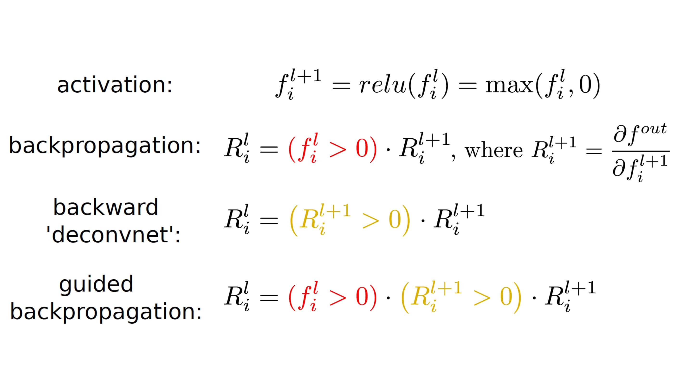
The most popularly used interpretability method is based on back-propagation of either gradients [Simonyan et al., 2014] or activation values [Bach et al., 2015]. This line of methods starts from the Saliency Map [Simonyan et al., 2014], which follows the normal gradient back-propagation process and constructs attributions by taking the absolute value of the partial derivative of the target output with respect to the input features , i.e., . Intuitively, the absolute value of the gradient indicates those input features that can be perturbed the least in order for the target output to change the most. However, the absolute value prevents the detection of positive and negative evidence that might be present in the input. To make the reconstructed heatmaps significantly more accurate for convolutional neural network (CNN) models, Deconvolution [Zeiler and Fergus, 2014a] and Guided Back-propagation [Springenberg et al., 2015] were proposed and these two methods and the Saliency Map method differ mainly in the way they handle back-propagation through the rectified linear (ReLU) non-linearity. As illustrated in Figure 1(a), for normal gradient back-propagation in the Saliency Map method, when the activation values in the lower layer are negative, the corresponding back-propagated gradients are masked out. In contrast, the Deconvolution method masks out the gradients when they themselves are negative, while the Guided Back-propagation approach combines these two methods: those gradients are masked out for which at least one of these two values is negative.
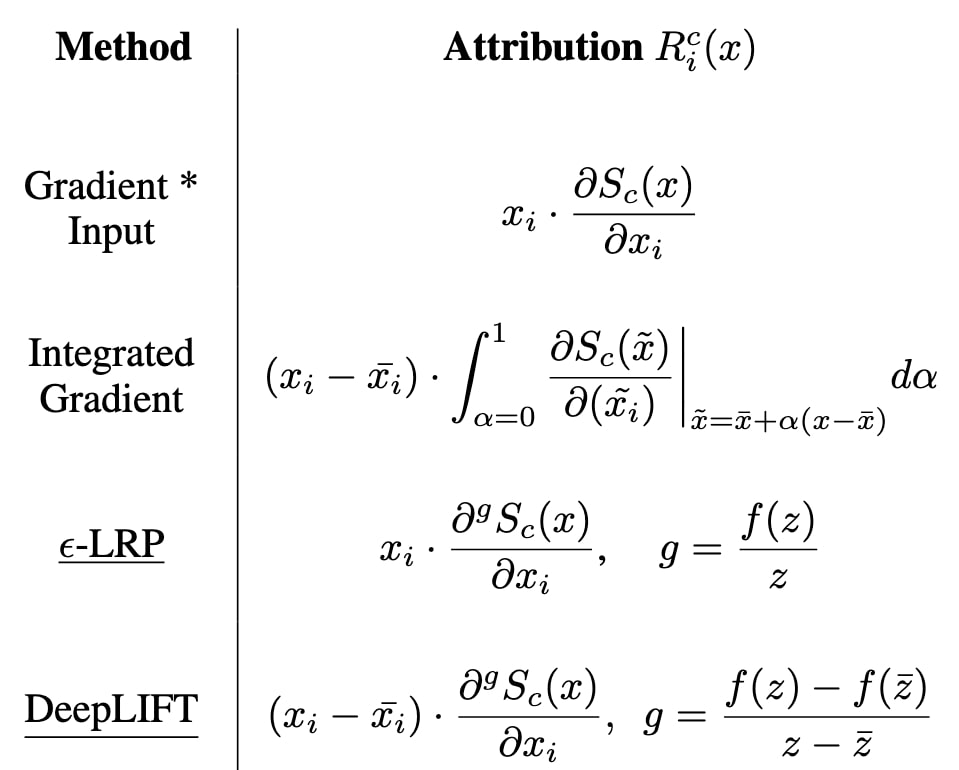
Gradient * Input [Shrikumar et al., 2017b] was proposed as a technique to improve the sharpness of the attribution maps. The attribution is computed taking the (signed) partial derivatives of the output with respect to the input and multiplying them with the input itself. Integrated Gradients [Sundararajan et al., 2017] is similar to Gradient * Input, with the main difference being that Integrated Gradients computes the average gradient as the input varies along a linear path from a baseline to . The baseline is defined by the user and often chosen to be zero. Please refer to Figure 1(b) for the mathematical definition for both methods.
Pixel-space gradient visualizations such as the above-mentioned Guided Back-propagation and Deconvolution are high-resolution and highlight fine-grained details in the image, but are not class-discriminative, i.e., the attribution value plots for different classes may look similar. In contrast, localization approaches like Class Activation Mapping (CAM) [Zhou et al., 2016] are highly class-discriminative (e.g., the ‘cat’ explanation exclusively highlights the ‘cat’ regions but not ‘dog’ regions in an image containing both a cat and dog). This approach modifies image classification CNN architectures by replacing fully-connected layers with convolutional layers and global average pooling, thus achieving class-specific feature maps. A drawback of CAM is that it requires feature maps to directly precede softmax layers, so it is only applicable to particular kinds of CNN architectures. To solve this shortcoming, Grad-CAM [Selvaraju et al., 2017] was introduced as a generalization to CAM, which uses the gradient information flowing into the last convolutional layer of the CNN to understand the importance of each neuron for a decision of interest. Furthermore, it is combined with existing pixel-space gradient visualizations to create Guided Grad-CAM visualizations that are both high-resolution and class-discriminative.
Besides gradients, back-propagation of activation values can also be leveraged as an interpretability approach. Layer-wise Relevance Propagation (LRP) [Bach et al., 2015] is the first to adopt this method, where the algorithm starts at the output layer and assigns the relevance of the target neuron equal to the output of the neuron itself (i.e., the activation value of the neuron) and the relevance of all other neurons to zero, as shown in Eq. 1. Then the recursive back-propagation rule (called the -rule) for the redistribution of a layer’s relevance to the preceding layer is described in Eq. 2, where we define to be the weighted activation of a neuron onto neuron in the next layer and the additive bias of unit . Once the back-propagation reaches the input layer, the final attributions are defined as . As an alternative, DeepLIFT [Shrikumar et al., 2017a] proceeds in a backward fashion similar to LRP but calibrates all relevance scores by subtracting reference values that are determined by running a forward pass through the network using the baseline as input and recording the activation of each unit. Although LRP and DeepLIFT were invented based on back-propagation of activation values, it has been demonstrated in [Ancona et al., 2018] that they can also be computed by applying the chain rule for gradients and the converted equations are summarized in Figure 1(b).
| (1) |
| (2) |
2.2 Feature perturbation
Compared to back-propagation based methods, which compute gradients of outputs with respect to input features, feature perturbation methods explicitly examine the change in model confidence resulting from occluding or ablating certain features.
The idea of masking parts of the input and measuring the model’s change in confidence was introduced in a model agnostic context, pre-DL by works such as [Štrumbelj et al., 2009] and [Robnik-Šikonja and Kononenko, 2008]. Based on some of these works, there have been multiple methods in DL for feature perturbation, attempting to explain the model based on the change in output classification confidence upon perturbation of features. These include model agnostic works based on conditional multivariate analysis and deep visualization [Zintgraf et al., 2017] (based on the instance-specific method known as prediction difference analysis) and explicit erasure of parts of input representations [Li et al., 2016]; as well as convolution neural network specific identification of image regions for which the model reacts most to perturbation [Zeiler and Fergus, 2014b] and image masking models that are trained to manipulate scores outputted by the predictive model by masking salient parts of the input image [Dabkowski and Gal, 2017]. Similar to image masking models, recent model-agnostic methods use generative models to sample plausible in-fills (as opposed to full masking) and optimize to find image regions that most change the classifier decision after in-filling [Chang et al., 2019].
In the direction of more theoretically grounded variable importance-based techniques, [Fisher et al., 2019] measure the model prediction difference upon adding noise to the features. Additionally, various adversarial perturbation techniques have been introduced that add noise to the feature representations, falling in the category of Evasion Attacks [Tabassi et al., 2019]. Evasion Attacks involve finding small input perturbations that cause large changes in the loss function and lead to mispredictions. These input perturbations are usually found by solving constrained optimization problems. These include gradient-based search algorithms like Limited-memory Broyden-Fletcher-Goldfarb-Shanno (L-BFGS) [Szegedy et al., 2013], Fast Gradient Sign Method (FGSM) [Goodfellow et al., 2015], Jacobian-based Saliency Map Attack (JSMA) [Papernot et al., 2016a] and Projected Gradient Descent (PGD) [Madry et al., 2018] among others. For detailed surveys on adversarial perturbation techniques in computer vision see [Akhtar and Mian, 2018]; for surveys on adversarial attacks in general see [Chakraborty et al., 2018] and [Yuan et al., 2019]. While the goal of these methods is to actively change model confidence for the purpose of attacking the model, they take advantage of the black box nature of DL models and have led to creation of techniques that can be used to deploy more robust and interpretable models.
2.3 Attention
Attention mechanisms have played an important role in model interpretations and the attention weights have been widely adopted as a proxy to explain a given model’s decision making [Xu et al., 2015, Xie et al., 2017, Clark et al., 2019, Voita et al., 2019].
Historically, attention mechanisms have been introduced in the context of sequence to sequence text model alignment as the way to directly incorporate the importance of the context to any given word representation. Each input word in a given context is represented by a weighted sum of the representations of other words. Naturally, the dynamic weights for each word can be interpreted as the contribution (or importance) of the words to a given word representation.
While the exact architecture of the attention-utilizing models differs from model to model, all of them make use of the set of computations known as the attention mechanism. The basic building block of attention is a generalized trainable function [Bahdanau et al., 2014, Vaswani et al., 2017]:
| (3) |
where and represent the context of a given element, the unmodified element contribution to the representation without the context being taken into an account, and the set of weights are the adaptable weights that represent the learned elements’ contributions.
The output of the Score function is known as the attention weights and represents the contributions of the other elements of the input to the representation of the given element or sequence as a whole; in the naive interpretation setting, a high post-training attention weight of an input feature or a set of features corresponds to a higher importance of the given feature value in producing a prediction.
Note that this methods of producing interpretation is intrinsically linked to the model itself and constitutes a direct interpretation of the outputs of the parts of a given attention-utilizing model (attention scores) as an explanation for the prediction. Since attention scores are often computed over already pooled representations of the elements and sequences, the element scores do not necessarily represent the direct feature contributions [Jain and Wallace, 2019, Brunner et al., 2019, Zhong et al., 2019].
The majority of work on attention based interpretability has been in the general time-series processing field due to both the success of the attention-using models and the natural idea of viewing the contribution of the other elements of the sequence to the current state [Sezer et al., 2020, Fawaz et al., 2019, Wang et al., 2019, Ardabili et al., 2019].
Fully-attention based models and attention based interpretations are also popular in natural language processing (NLP) due to the compositional nature of syntax and meaning [Wolf et al., 2020].
2.4 Model distillation
Model distillation (also known as Network distillation) is a model compression technique where a simpler model (student) is “taught” by a more complex model (teacher). While the original use of the technique focused on the improved performance or compactness of the student model [Hinton et al., 2015], it is important to note that if the simpler model is naturally interpretable, the transfer results in an “interpretable” model explaining the behavior of the more complex teacher model.
A complex model’s behavior may be approximated either locally, by fitting a simpler model around a given example to produce an explanation for a given point [Ribeiro et al., 2016a], or globally, by fitting one simple model directly to the teacher model, using all the training data [Lakkaraju et al., 2017].
Due to the explicit “interpretation” use case of the technique, the student models are in general limited to either generalized linear models [Ribeiro et al., 2016a], decision trees [Craven and Shavlik, 1995, Schmitz et al., 1999, Plumb et al., 2018] or direct rules or set inductions [Sethi et al., 2012, Lakkaraju et al., 2017, Ribeiro et al., 2018, Zilke et al., 2016]
The most influential member of this family of interpretation producing techniques is LIME [Ribeiro et al., 2016a], a general method for generating local explanation for a specific input case. The local model that serves as an explanation for a given point is obtained by minimizing
| (4) |
where is a class of the interpretable models used to produce an explanation, defines the neighborhood of points near , is the measure of the difference between the original model and the explanation model prediction in that neighborhood, and is a complexity measure of the explanation model.
In practice, in the classical LIME use, is set to be the distance weighted squared loss between the original model and the explanation model prediction computed over a randomly sampled set of data points biased to lie near by . The explanation model class is the class of all linear models and is a regularization term to prevent overfitting.
The vast majority of local knowledge distillation for interpretability models are the result of modifying Lime in either the neighborhood construction (ALIME [Shankaranarayana and Runje, 2019]), sampling (MPS-LIME [Shi et al., 2020]) and input structure constraining procedure (GraphLime [Huang et al., 2020]) or the nature of the explanation model (SurvLIME [Kovalev et al., 2020], GRAPHLime [Huang et al., 2020]). Another popular trend is producing semi-global explanation models through LIME-like fitting procedures (LIME-SUP [Hu et al., 2018], Klime [Hall et al., 2017], NormLime [Ahern et al., 2019], DLIME [Zafar and Khan, 2019], ILIME [Shawi et al., 2019]).
2.5 Game theory based Interpretability Methods
DL models can also be interpreted via Shapley value, a game theory concept inspired by local surrogate models [Lundberg and Lee, 2017]. Shapley value is a concept of fair distribution of gains and losses to several unequal players in a cooperative game [Shapley, 1953]. It is an average value of all marginal contributions to all possible interactions of features (i.e., players in the game) given a particular example. Therefore, the Shapley value can explain how feature values contribute to the model prediction of the given example by comparing against the average prediction for the whole dataset. Nevertheless, the Shapley value approximation is not easy to compute when the learning model becomes complicated.
Recently, researchers proposed a unified framework, SHAP (SHapley Additive exPlanations) values, to approximate the classical Shapley values with conditional expectations for various kinds of machine learning models, which include linear models, tree models [Lundberg et al., 2018a], and even complicated deep neural networks [Lundberg and Lee, 2017]. SHAP has been widely used recently for DL interpretation, yet researchers also admit to concerns about this popular interpretability method.
First, the SHAP for neural networks (KernelSHAP) is based on an assumption of model linearity. To mitigate the problem, [Ancona et al., 2019] propose a polynomial-time approximation algorithm of Shapley values, Deep Approximate Shapley Propagation (DASP), to learn a better Shapley value approximation in non-linear models, especially deeper neural networks. DASP is a perturbation-based method using uncertainty propagation in the neural networks. It requires a polynomial number of network evaluations, which is faster than other sampling-based methods, without losing approximation performance. Also, [Sundararajan and Najmi, 2020] show that SHAP, or other methods using Shapley values with conditional expectations, can be sensitive to data sparsity and yield counterintuitive attributions that make an incorrect model interpretation. They propose a technique, Baseline Shapley, to provide a good unique result.
2.6 Example based Interpretability Methods
Instead of explaining the model using the attributive contribution of input data points, example based methods interpret the model behavior using only the particular training data points that are representative or influential for the model prediction.
For DL models, there are several interpretation methods based on example-level information. For example, the influence function [Koh and Liang, 2017], example-level feature selection [Chen et al., 2018], contextual decomposition (CD) [Murdoch et al., 2018], and the combination of both prototypes and criticism samples—data points that can’t be represented by prototypes [Kim et al., 2016]. Other popular methods for interpretation, such as LIME [Ribeiro et al., 2016a] (Section 2.4) and SHAP [Lundberg and Lee, 2017] (Section 2.5), also provide example-level model interpretability.
The influence function is an example of example-based interpretability [Koh and Liang, 2017], which can be used in both computer vision [Koh and Liang, 2017], and NLP [Han et al., 2020b]. The goal of the influence function is to measure the change in the loss function as we add a small perturbation, weight, or remove a influence instance, which is a representative, influential training point. Under the smoothness assumptions, the influence function can be computed using the inverse of the Hessian matrix of the loss function or by using the Hessian-vector products to approximate the result. The influence function can also be used to generate an adversarial attack.
Researchers developed DL-based instance-wise feature selection at the example-level for feature importance measurement [Chen et al., 2018]. Instance-wise feature selection (L2X, Learning to Explain) measures feature importance locally for each specific example and therefore indicates which features are the key for the model to make its prediction on that instance. L2X is trained to maximize the mutual information between selected features and the response variable, where the conditional distribution of the response variable given the input is the model to be explained. To solve an intractable issue of direct estimation of mutual information and discrete feature subset sampling, the authors apply a variational approximation for mutual information, then develop a continuous reparameterization of the sampling distribution. The method has been applied to CNN and hierarchical long short-term memory (LSTM) on different datasets and yields a better explanation performance quantitatively and qualitatively.
CD is an interpretation method to analyze individual predictions by decomposing the output of LSTMs without any changes to the underlying model [Murdoch et al., 2018]. In NLP, it decomposes an LSTM into a sum of two contributions: those resulting solely from the given phrase and those involving other factors. CD captures the contributions of combinations of words or variables to the final prediction of an LSTM. In the study, researchers demonstrate that CD can explain both NLP and general LSTM applications. For example, they model for sentiment analysis by identifying words and phrases of differing sentiment within a given review and extracting positive and negative words from the model. The CD method can be further extended to a more general version, contextual decomposition explanation penalization (CDEP) [Rieger et al., 2020]. CDEP is a method that allows the insertion of domain knowledge into a model to ignore spurious correlations, correct errors and generalize to different types of dataset shifts. It is general and can be applied to different neural network architectures.
For graph neural networks, [Ying et al., 2019] further propose a model-agnostic GnnExplainer to provide interpretability on graph-based tasks, such as node and graph classification. By identifying the prediction-relevant edges, GnnExplainer can highlight local subgraph structures and small subsets of important features to the prediction. The method can be used for single and multiple instance explanations in a graph.
To tackle the real-world data, which may not have a set of prototypical examples representing the data well, we can also utilize both the prototypical examples and criticism samples that don’t fit the model well [Kim et al., 2016]. The MMD-critic (maximum mean discrepancy-critic) method uses a Bayesian approach to select the prototype and criticism samples and to provide explanations that can facilitate human reasoning and understanding of the model.
2.7 Generative based Interpretability Methods
The basis of generative based methods for explaining a model’s behavior uses information that does not occur explicitly in attributes of the input, but is derived from external knowledge sources, from a causal model, or from explainable probabilistic modeling.
For example, the state-of-the-art general domain neural question answering (QA) system attempts to provide human-understandable explanations for better commonsense reasoning, yet to interpret how the model utilizes common sense knowledge, a common-sense explanation generation framework is required [Rajani et al., 2019]. Researchers collect human narrative explanations for common sense reasoning and pretrain language models [Rajani et al., 2019], which can generate explanations and be used concurrently with the QA system (Commonsense Auto-Generated Explanations (CAGE) framework). They further transfer knowledge (generated explanations) to out-of-domain tasks and demonstrate the capacity of pretrained language models for common sense reasoning.
Generative Explanation Framework (GEF) is another hybrid generative-discriminative method that explicitly captures the information inferred from raw texts, generates abstractive, fine-grained explanations (attributes), and simultaneously conducts classification tasks. It can interpret the predicted classification results and improve the overall performance at the same time [Liu et al., 2019]. More specifically, the authors introduce the explainable factor (EF) and the minimum risk training (MRT) approach that learn to generate more reasonable explanations. They pretrain a classifier using explanations as inputs to classify texts, then adopt the classifier to jointly train a text encoder by computing EF, which is the semantic distance between generated explanations, gold standard explanations, and inputs, and then minimizing MRT loss that considers both the distance between predicted overall labels and ground truth labels, as well as the semantic distance represented in EF. GEF is a model-agnostic method that can be used in different neural network architectures.
[Madumal et al., 2020] introduced action influence models that utilize the structural causal model to generate the explanation of the behavior of model-free reinforcement learning agents through knowing the cause-effect relationships using counterfactual analysis. The proposed model has been evaluated on deep reinforcement learning algorithms, such as Deep Q Network (DQN) [Mnih et al., 2013], Double DQN (DDQN) [Van Hasselt et al., 2016], Proximal Policy Optimization (PPO) [Schulman et al., 2017], and Advantage Actor Critic (A2C) [Mnih et al., 2016].
[Wisdom et al., 2016] developed a model-based interpretation method, sequential iterative soft-thresholding algorithm (SISTA), to construct recurrent neural network (RNN) without black-box components like LSTMs, via the trained weights of the explicit probabilistic model.
3 Methods for Interpretability in Healthcare
In the last section, we have summarized the methodology for each class of interpretation methods. Most of these methods were initially proposed for general domain applications. In order to deploy them to healthcare problems, some customization needs to be performed. Therefore in this section, we discuss how each class of interpretation methods can be adapted to healthcare systems. We also discuss what kinds of clinical/medical observations and findings we can make with the help of these interpretation methods.
3.1 Back-propagation
Back-propagation based interpretability methods have been widely used to help visualize and analyze those DL models adopted for healthcare problems, which include computer vision, NLP [Gehrmann et al., 2018], time series analysis, and static features-based predictive modeling. We would like to summarize these successful applications and categorize them based on the applied task types.
In computer vision tasks, many powerful DL models have achieved close to expert doctor performance [Esteva et al., 2017, Ran et al., 2020] and thus it is very meaningful to study how these models can accomplish such great success [Singh et al., 2020b]. [Xie et al., 2019] adopted CAM [Zhou et al., 2016] to generate heatmaps separately for melanoma and nevus cells in skin cancer histology images so that the morphological difference between these two types of cells can be visualized: the melanoma cells are of irregular shape and the nevus cells are distinctly shaped and regularly distributed. [Zhang et al., 2021] used Grad-CAM to provide an explainable heatmap for an attention network built for classifying chest CT images for COVID-19 diagnosis, while Grad-CAM was also used to explain a graph convolutional network for secondary pulmonary tuberculosis diagnosis based on chest CT images [Wang et al., 2021]. Integrated Gradients [Sundararajan et al., 2017] was used to visualize the features of a CNN model used for classifying estrogen receptor status from breast magnetic resonance imaging (MRI) images [Pereira et al., 2018], where the model was found to have learned relevant features in both spatial and dynamic domains with different contributions from both. Overall, back-propagation based methods have been used to visualize and interpret various medical imaging modalities such as brain MRI [Eitel et al., 2019], retinal imaging [Sayres et al., 2019, Singh et al., 2020a], breast imaging [Papanastasopoulos et al., 2020, Kim et al., 2018], skin imaging [Young et al., 2019], computed tomography (CT) scans [Couteaux et al., 2019], and chest X-rays [Linda, 2020].
For features-based predictive modeling, back-propagation based interpretability methods can be applied to both static and time-series analysis. For static analysis (e.g., therapy recommendation based on a fixed set of features), fully connected neural networks are typically utilized for modeling and thus are the target to be interpreted. Commonly-used interpretability methods include DeepLIFT [Fiosina et al., 2020], LRP [Li et al., 2018, Zihni et al., 2020], etc. For time-series analysis, besides being able to analyze which features are more important or relevant to the prediction among all features used [Yang et al., 2018], it is noteworthy that we can also analyze what temporal patterns are more influential to the final model decision [Mayampurath et al., 2019, Suresh et al., 2017].
3.2 Feature perturbation
Feature perturbation methods have primarily been discussed in the context of adversarial attacks in the healthcare domain [Finlayson et al., 2019a], mainly as potential future risks due to the ready acceptance of machine learning in diagnosis and insurance claims approval. Nevertheless, the features that are most influential if altered by an attacker are also the ones to which the model’s responses are most sensitive [Finlayson et al., 2019a].
[Finlayson et al., 2019b] perform adversarial perturbations (a variation on FGSM attack [Goodfellow et al., 2015]) by addition of gradient-based noise to three highly accurate deep learning systems for medical imaging. By attacking models that classify diabetic retinopathy, pneumothorax and melanoma, they show vulnerabilities in three of the most highly visible successes for medical deep learning. In addition, they discuss hypothetical scenarios of how attackers could take advantage of the vulnerabilities the systems demonstrate. More broadly, they comment on industries and scenarios that could be affected by adversarial attacks in the future: insurance fraud and determining pharmaceutical and device approvals. They discuss the challenging tradeoff between forestalling approval until a resilient algorithm is built and the harm that delaying the deployment of a technology impacting healthcare delivery for millions could entail.
[Iqtidar Newaz et al., 2020] show vulnerability in smart healthcare systems (SHS) by manipulating device readings to alter patient status. By performing two types of attacks, including Evasion Attacks [Tabassi et al., 2019], they identify flaws in an underlying ML model in a SHS. Employing feature perturbation methods such as FGSM [Goodfellow et al., 2015], randomized gradient-free attacks based on [Carlini and Wagner, 2017], [Croce et al., 2019], and [Croce and Hein, 2018] and zeroth order optimization based attacks [Chen et al., 2017], they are able to alter patient status for ML models based on patient vital signs.
[Chen et al., 2020] generate adversarial examples based on perturbation techniques for electrocardiograms. They use techniques from [Carlini and Wagner, 2017] and [Athalye et al., 2018] to misguide arrhythmia classification. In a similar application, [Han et al., 2020a] introduce a smooth method for perturbing input features to misclassify arrhythmia.
For temporal data in EHR, [Sun et al., 2018] introduce an optimization based attack strategy, similar to [Chen et al., 2017], to perturb EHR input data. [An et al., 2019] introduce a JSMA and attention-based attack by jointly modeling the saliency map and attention mechanism. Finally, in a domain agnostic setting, [Naseer et al., 2019] introduce cross-domain transferability of adversarial perturbations using a generative adversarial network (GAN)-based framework. They show how networks trained on medical imaging datasets can be used to fool ImageNet based classifiers. Successful transferability of adversarial perturbations can make it even simpler to fool healthcare models across multiple task domains, and potentially modalities. One such paper examines the effect of universal adversarial perturbations in the medical imaging space [Hirano et al., 2021].
Several methods have been proposed in the general domain to counter these adversarial attacks, namely proactive defense ([Cisse et al., 2017, Gu and Rigazio, 2014, Papernot et al., 2016b], [Shaham et al., 2018]) and reactive defense ([Feinman et al., 2017, Grosse et al., 2017, Lu et al., 2017]). Proactive defense methods increase the robustness of models retroactively, whereas reactive defense models detect the adversarial examples. There are also other methods, such as using collaborative multi-task learning ([Wang et al., 2020]). While it may seem that the possibility of adversarial perturbations works against the recommendation of using deep learning in healthcare settings, there are recent works pushing the boundaries by actively examining the reasons for the susceptibility of healthcare data to attacks ([Ma et al., 2021]). Since feature perturbation techniques have strong policy-level implications in healthcare, it is also imperative to tailor general domain defense methods to the healthcare setting.
3.3 Attention
Attention architectures designed with a special consideration for interpretability are routinely used for EHR-based longitudinal prediction tasks such as heart failure prediction [Choi et al., 2016, Kaji et al., 2019], sepsis [Kaji et al., 2019], intensive care unit (ICU) mortality [Shi et al., 2019], automated diagnosis, and disease progression modeling [Gao et al., 2019, Mullenbach et al., 2018, Ma et al., 2017, Bai et al., 2018, Alaa and van der Schaar, 2019]. The underlying representation of such a model is often produced by an LSTM variant with the attention used to compute the contribution of a given feature or time step element of the sequence to the prediction. The best known model of this kind is RETAIN [Choi et al., 2016], which includes computing the attention weights over both the time-step of the time-series and the individual features of the inputs.
Pure attention-based architectures such as the Transformer have revolutionized NLP-based modeling, allowing the use of massive unlabeled medical text for pretraining [Lee et al., 2020, Alsentzer et al., 2019, Beltagy et al., 2019]. Adoption of such models for non-text data is still relatively rare [Li et al., 2020b, Rajan et al., 2017].
A special variant of the attention mechanism that seeks to address interpretability allows the model to output uncertainty on each input feature and use the aggregated uncertainty information for prediction [Heo et al., 2018].
Despite the widespread use of the attention maps as explanations, we would caution against the direct interpretation of attention as an element’s contributions to the prediction in the medical domain. More studies are needed to disentangle self-attention produced representations from the context contribution itself.
3.4 Model distillation
LIME [Ribeiro et al., 2016a] is one of the most popular techniques used to produce instance-level explanations for black-box model predictions in medical AI. The model-agnostic nature of the technique has led to its use in a diverse set of longitudinal EHR-based prediction tasks such as heart failure prediction [Khedkar et al., 2020], cancer type and severity inferences [Moreira et al., 2020], breast cancer survival prediction [Hendriks et al., 2020], and predicting development of hypertension [Elshawi et al., 2019].
It should be noted that the LIME variants are not widely used, despite the potential clinical usefulness of such interpretation methods. Among the potentially useful variants for ML in medicine are SurvLIME [Kovalev et al., 2020], introduced specifically for producing Cox proportional hazards explanations for black-box survival models, and DLIME [Zafar and Khan, 2019], a hierarchical clustering neighborhood based semi-global LIME variant for producing more consistent explanations for predictions over similar inputs.
3.5 Game theory based Interpretability
The game theory based SHAP algorithm has been widely applied in the medical domain for feature contribution analysis due to its ability to explain not only individual predictions but also global model behavior via the aggregation of Shapley values. SHAP is also model-agnostic, so that it can be applied to various machine learning algorithms [Lundberg and Lee, 2017, Lundberg et al., 2018b].
In the direct usage of SHAP for deep learning in healthcare, [Arcadu et al., 2019] applied SHAP to find the crucial regions, which are peripheral fields, for identifying diabetic retinopathy progression. Also, for the interpretation of medical imaging, [Young et al., 2019] and [Pianpanit et al., 2019] utilized KernelSHAP to generate the saliency maps for interpreting the deep neural networks for melanoma prediction and Parkinson’s disease prediction, respectively. [Levy et al., 2019] also adopted SHAP to interpret the portal region prediction in pathology slide imaging. Beyond medical imaging, [Boshra et al., 2019] used SHAP to investigate the features’ influence on concussion identification given the electroencephalography (EEG) signals.
[Ancona et al., 2019] uses the DASP algorithm to approximate the Shapley values and yields the explanation of the deep learning models and applies it to a fully-connected network model for predicting the Parkinson’s disease rating scale (UPDRS), which is a regression task to predict the severity of Parkinson’s disease based on 18 clinical features in a telemonitoring dataset.
In [Lundberg et al., 2018b], they also have anesthesiologists consulted to ensure that their model explanations are clinically meaningful. The anesthesiologists were asked to justify the SHAP explanations with the change in model output when a feature is perturbed. [Li et al., 2020a] also shows that it is possible to use SHAP for modeling and visualizing nonlinear relationship between prostate-specific antigen and Gleason score in prostate cancer that is consistent with the prior knowledge in the medical literature. Such clinical evaluations help the medical community to accept the interpretation method better.
Other works mentioned in this section also provide explanations that are aligned with prior knowledge and ground truth given by the dataset via visualization or computing quantitative metrics, yet none of them are justified by a formal clinical user study. Further study is needed for these methods and applications in healthcare.
One major concern of using SHAP in the medical domain is that the Shapley value and SHAP was originally derived from economics tasks, where the cost is additive. However, clinical features are usually heterogeneous, and the Shapley values derived from the model may not be meaningful in the domain [Kovalerchuk et al., 2021]. Further investigation is needed to justify real-world clinical use of SHAP-based interpretations.
3.6 Example based Interpretability
Example-based model interpretation provides a mental model that allows clinicians to refer to some similar cases, prototypes, or clusters given a new case.
Researchers utilize CDEP to ignore spurious confounders in skin cancer diagnosis [Rieger et al., 2020]. The study uses a publicly available image dataset from ISIC (International Skin Imaging Collaboration), which has colorful patches present in approximately 50% of the non-cancerous images but not in the cancerous images. It can be problematic if the learned model uses such spurious patch features as an indicator but not the critical underlying information for skin cancer prediction. The CDEP helps penalize the patches for having zero importance during training and mitigates the issue.
Although yielding better model performance with a quasi-explanation with a skin cancer classification example, CDEP has not yet been justified by a formal clinical user study and not yet been accepted by the medical community. It is still at the research rather than the deployment stage.
3.7 Generative based Interpretability
DL interpretability can also be learned based on expert-interpretable features provided during the learning process.
To provide visually interpretable evidence for breast cancer diagnostic decisions, [Kim et al., 2018] developed an interpretability framework that includes a breast imaging reporting and data system (BIRADS) guided diagnosis network and a BIRADS critic network. The interpretable 2D BIRADS guide map, which is generated from the visual feature encoder, can help the diagnosis network focus on the critical areas related to the human-understandable BIRADS lexicon via the critic network.
The study shows that with the BIRADS guide map, the performance is significantly higher than the network without the guide map. This finding also indicates the critical role and necessity of integrating medical domain knowledge while deploying machine learning models in healthcare.
For radiology, [Shen et al., 2019] proposed an interpretable deep hierarchical semantic convolutional neural network (HSCNN) for pulmonary nodule malignancy prediction on CT images. HSCNN generates the binarized low-level expert-interpretable diagnostic semantic features that are commonly used by radiologists, such as sphericity, margin, and calcification; these are inputs to the high-level classification model, along with the latent representations learned from the visual encoder.
Both [Kim et al., 2018] and [Shen et al., 2019] demonstrate that the image guide map and label generation process may help clinicians curate the raw image information to high-level diagnostic criteria, yet the method is not yet justified by formal clinical user studies. Further study is needed for these methods to be accepted by the medical community.
4 Discussion
4.1 Dimensions of different interpretability methods
The current literature presents several different classification schemes for interpretation methods in DL [Lipton, 2018, Doshi-Velez and Kim, 2017, Pedreschi et al., 2019]. In addition to the methodology motivated classification used in the Interpretability methods section of the paper, we present two different questions that every interpretation producing method naturally poses:
-
1.
Model Dependence: Does the explanation model depend on the internal structure of the model it is explaining or can it be used for producing an explanation of any “black-box” model?
-
2.
Explanation Scope: Does the explanation model focus on producing an explanation for a given input-prediction pair or is it attempting to create a unified global explanation of the model’s behavior?
A characterization of the most commonly used methods to produce interpretations in health care with respect to these aspects is presented in Table 1.
In general, the vast majority of the methods are explicitly local, producing the explanation for a given decision only, with some attempts at aggregation of the local explanation into patterns [Ramamurthy et al., 2020, Lakkaraju et al., 2019].
The community appears to be deeply split on the issue of model dependence, with the proponents citing the necessity of explanation fidelity [Rudin, 2019], while opponents doubt the inherent fidelity of the directly model-dependent explanations [Jacovi and Goldberg, 2020] and stress the need for flexible model-independent explanation methods [Ribeiro et al., 2016b].
| Class: | Model | Scope | Dep. | Potential Issues | Ref. |
| Back-prop. | Integrated Gradients | L | I | More computationally expensive than Gradients * Inputs, the baseline needs to be carefully selected/tuned for some cases | [Sundararajan et al., 2017] |
| CAM | L | I | Label/class discriminative features revealed by this method may not be convincing and accurate for some data samples | [Zhou et al., 2016] | |
| LRP | L | I | Initially proposed for interpreting multi-layer perceptions and hard to generalize well to more complex neural networks such as LSTM and Transformers | [Bach et al., 2015] | |
| Feat perturbation | Prediction Difference Analysis | L | I | Computationally expensive. Simulates the absence of feature via marginalization, rather than exact knowledge of model behavior without the feature present. | [Zintgraf et al., 2017] |
| Representation Erasure | G | I | Computationally expensive, requires several steps of probing. Injects random noise into input for representation erasure. | [Li et al., 2016] | |
| Counterfactual Generation | L | I | Computationally expensive due to intermediate generative stage for injecting noise respecting data distribution. Involves similar marginalization approximations as Prediction Difference Analysis. | [Chang et al., 2019] | |
| Attention | RETAIN | L | D | Attention weight correspond to the importance of the intermediate representations to the final representation, not the input elements directly. | [Choi et al., 2016] |
| Attend and Diagnose | L | D | Same issues as retain, exacerbated by the use of the fully-additional architecture of the model | [Rajan et al., 2017] | |
| Model distillation | LIME | L | D | The explanation is not cross instances consistent and might vary wildly for even for very similar instances. Possible issues on discontinuous data. Might produce inconsistent results across the multiple runs | [Ribeiro et al., 2016a] |
| Anchors | S | I | Might produce inconsistent results across multiple runs. The explanation might be too specific and not very robust at the decision boundary | [Ribeiro et al., 2018] | |
| Game theory | SHAP | L | I | Computationally expensive. Require the access to training data for interpretation. | [Lundberg and Lee, 2017] |
| Example | Influence function | L | I | Won’t work for models without differentiable parameters and losses. Only an approximation. No clear cut of “influential” and “non-influential”. May not be human-interpretable if there are too many feature values in a prototype. | [Koh and Liang, 2017] |
| Contextual decomposition | L | D | Only for LSTM. Require further algorithm modifications to extend the method for other network architecture. | [Murdoch et al., 2018] | |
| Generative | CAGE | L | D | Require high-quality external knowledge resources. Task-specific method. | [Rajani et al., 2019] |
4.2 Credibility and Trustworthiness of Interpretability Methods
In this section we will discuss two aspects of the methods used to produce interpretations of decision models used in health care:
-
1.
How faithful is the interpretation to the underlying decision making model?
-
2.
How understandable are the interpretations to human expert users?
The two aspects are often at odds with each other: A complex model decision might require a rather complex explanation to cover all of the possible aspects of the model’s behaviors on different inputs, which might not look easy to understand to humans.
4.2.1 Faithfulness of the interpretation
We first discuss the direct correspondence between the produced interpretation and the model’s decision making, known in the literature under the terms Fidelity [Jacovi and Goldberg, 2020] or Faithfulness [Rudin, 2019]. A perfectly faithful interpretation accurately represents the decision making of the model being explained. If the interpretation is constrained to agree with the model’s behavior on all possible inputs, then no simpler explanation than the original model is possible. Even model dependent explanation producing methods may not be faithful to the original model because, as a simplified model, they may not include all parts of the original decision making process [Jain and Wallace, 2019].
When using an explanation producing model for black-box models trained on complex healthcare data, we recommend the user to consider the following issues to gain more insight into the explanation model’s faithfulness.
-
1.
For explanations that, in themselves, are predictive models, look at the prediction agreement between the explanation model and the original: if the concordance is low, then the model is not faithful.
-
2.
While it is hard to estimate the fidelity of an explanation method, consider computing recently proposed fidelity measures over the set of the explanation methods you are planning to use [Yeh et al., 2019].
-
3.
Consider running “feature occlusion” sanity checks, to check if changing those model elements according to the explanation change the original predictions [Hooker et al., 2018].
-
4.
Due to the nature of some interpretation producing models, the same model might produce different explanations for the same pair of input-outputs over multiple runs.
4.2.2 Plausibility of the interpretation as defined by the expert user
Traditionally, clinicians tend to embrace expert-curated models, such as the APACHE (Acute Physiology and Chronic Health Evaluation) score for evaluating the patient severity in the ICU [Knaus et al., 1985], due to the consistency between used model features and domain knowledge. In contrast, machine learning approaches for healthcare problems aim to further improve performance by learning a much more complex representations from raw features while sacrificing model transparency. Machine learning interpretability methods may provide human-understandable explanations, yet it is crucial that the explanations should be aligned with our knowledge to be trustable, especially for real-world deployment in the healthcare domain. However, current deployments with interpretability methods mainly focus only on helping to debug the model for engineers, but not the real-world use for end users [Bhatt et al., 2020b]. The appropriate interpretability methods should be selected and evaluated both to help model developers (data scientists and machine learning practitioners) understand how their models behave, and to assist clinicians to understand the rationale for model predictions for decision making.
For model developers, researchers evaluate their use of interpretability methods with different levels of model transparency (generalized additive models (GAMs) and SHAP), from both quantitative (machine-learned interpretability) and qualitative (visualization) perspectives using interviews and surveys [Kaur et al., 2020]. The results, however, show that developers usually over-trust the methods and this may lead to their misuse, especially over-relying on their “thinking fast (system 1)” [Kahneman, 2011] since the good visualization may sway human thought, but may not fully explain the behavior of the system and may be incorrectly interpreted by developers. Moreover, visualization sometimes is not able to be fully understood and interpreted correctly by the model developers. The authors point out that developers usually just focus on superficial values for model debugging instead of using explanations to dig deeper into data or model problems. They also enumerate the common issues faced by developers, which include missing values, data change over time, data duplication, redundant features, ad-hoc categorization, and difficulties of debugging the methods based on explanations. The developers are also shown to be biased toward model deployment even after recognizing suspicious aspects of the models.
From a clinical perspective, it is necessary and critical to have clinically relevant features that align with medical knowledge and clinical practice [Caruana et al., 2015], while under-performing models may still be acceptable as long as the errors are explainable. In [Tonekaboni et al., 2019b], the authors survey clinicians in the ICU and emergency department to understand the clinicians’ need for explanation, which is mainly to justify their clinical decision-making to patients and colleagues.
Depending on the problem scope, different levels of interpretability may be considered by clinicians. [Elshawi et al., 2019] conduct a case study of the hypertension risk prediction problem using the random forest algorithm and explore the important factors with different model-agnostic interpretability techniques at either global or local-level interpretation. They find that different interpretability methods in general provide insights from different perspectives to assist clinicians to have a better understanding of the model behavior depending on clinical applications. Global methods can generalize over the whole cohort while local methods show the explanation for specific instances. Thus, applications such as the hypertension risk prediction problem may focus on global risk factors derived from either global interpretability methods, mainly non-DL based techniques such as feature importance and partial dependence plot, or the aggregation of local explainers (e.g. SHAP, LIME) [Elshawi et al., 2019], while disease progression prediction requires integrated interpretations at local, cohort-specific and global levels [Ahmad et al., 2018].
However, different interpretability methods may yield a different subset of clinically relevant important features due to their ways to obtain feature importance. For instance, SHAP, coefficient of regression models, and permutation-based feature importance may provide completely different interpretations even if they are all at the global level. With some clinical examples, researchers found that the local interpretation methods (LIME and SHAP) of the correctly predicted samples are in general intuitive and follow common patterns, yet for the incorrectly predicted cases (either false positive or false negative cases), these local methods can be less consistent and more difficult to interpret [Elshawi et al., 2019]. Nevertheless, the users may not be aware of the assumption of using the model and how it makes the decision: e.g., the additivity assumption of the SHAP algorithm. Interpretability can be quite subjective, and the computerized techniques for producing interpretations lack the interactivity that is often crucial when one human expert is trying to convince another [Lahav et al., 2018].
Studies also show shortcomings of some interpretability methods while adopting them for real-world clinical settings [Tonekaboni et al., 2019b, Elshawi et al., 2019]. For example, the complex correlation between features in feature importance-based methods, the weak correlation between feature importance and learned attention weights for recurrent neural encoders [Jain and Wallace, 2019], and the trade-off between performance and explainability for rule-based methods, are all potential problems of using global interpretability methods [Tonekaboni et al., 2019b]. For local interpretability methods, researchers also show that clinicians can easily conclude the explanation at the feature-level using LIME, but the main problem is that the LIME explanation can be quite unstable, where patients with similar patterns may have very different interpretations [Elshawi et al., 2019]. Instead, the advantage of the Shapley value interpretation method is that it makes the instance prediction considering all feature values of the instance, and therefore the patients with similar feature values will also have similar interpretations [Elshawi et al., 2019]. But the cons of Shapley value-based methods are that they can be computationally expensive and that they need to access the training data while building model explainers [Lundberg and Lee, 2017, Janzing et al., 2020].
It is not trivial to select appropriate interpretability methods for real-world healthcare applications. Researchers therefore provide a list of metrics, including identity, stability, separability, similarity, time, bias detection and trust, to evaluate different interpretability methods when considering real-world deployment [ElShawi et al., 2020]. However, they find that there is no consistent winning method for all metrics across various interpretability methods, such as LIME, SHAP and Anchors. Thus, it is essential to make a clear plan and think more about the clinical application and interpretability focus in order to select the reasonable and effective interpretability methods and metrics for real-world use.
To further achieve the potential clinical impact of deployed models, we should not only focus on advancing machine learning techniques, but also need to consider human-computer interaction (HCI), which investigates complex systems from the user viewpoint, and propose better designs to bridge the gap between users and machines. End users’ involvement in the design of machine learning tools is also critical to understand the skills and real needs of end users and how they will utilize the model outputs [Ahmad et al., 2018, Feng and Boyd-Graber, 2019]. [Kaur et al., 2020] suggest that it may be beneficial to design interpretability tools that allow back-and-forth communication (human-in-the-loop) to make interpretability a bidirectional exploration, and also to build tools that can activate thinking via “system 2” for deeper reasoning [Kahneman, 2011].
4.3 Benchmarking Interpretation Methods
Now we have many different kinds of interpretation methods to choose when we want to analyze a neural model, although they are still in need of further improvement. At the current state of the art, which method we should choose still does not have a definite answer. The choice of the right interpretation method should depend on the specific model type we want to interpret; however, such a detailed and comprehensive guideline for all kinds of models to be analyzed is currently not available. Several recent studies started to look into this problem by benchmarking some popularly used interpretation methods applied to some neural models such as CNN, RNN, and transformer. For example, [Arras et al., 2019] first use four interpretation methods, namely LRP, Gradient*Input, occlusion-based explanation [Li et al., 2016], and CD [Murdoch et al., 2018], to obtain the relevance scores of each word in the text for the LSTM model for text classification tasks, and then measure the change of accuracy after removing two or three words in decreasing order of their relevance. By comparing the percentage of accuracy decrement, they observe that LRP and CD perform on-par with the occlusion-based relevance, with near 100% accuracy change, followed by Gradient*Input which leads to only 66% accuracy change. This experiment indicates that LRP, CD, and occlusion-based methods can better identify the most relevant words than Gradient*Input. As a counterpart, [Ismail et al., 2020] argue that one should not compare interpretation methods solely on the loss of accuracy after masking since the removal of two or three features may not be sufficient for the model to behave incorrectly. Instead, they choose to measure the precision and recall of features identified as salient by comparing against ground truth important features and report the weighted precision and recall as the benchmarking metric. However, their annotations of which features are important are synthesized rather than collected by human annotation, which is not that convincing. In a more theoretical way, [Bhatt et al., 2020a] propose several equations as quantitative evaluation criteria to measure and compare the sensitivity, faithfulness, and complexity of feature-based explanation methods.
Through these benchmarking evaluations, we find that different interpretation methods may vary a lot in their advantages and disadvantages. To make use of this fact, some studies propose to aggregate two kinds of interpretation methods so that they can complement each other [Ismail et al., 2020]. For instance, [Bhatt et al., 2020a] develop an aggregation scheme for learning combinations of various explanation functions, and devise schemes to learn explanations with lower complexity and lower sensitivity. We hope to see more efforts along this direction to generalize such an aggregation scheme to a broader range of interpretation methods.
5 Conclusion
In this review, we provided a broad overview of interpretation methods for interpreting the black-box DL models deployed for healthcare problems. We started by summarizing the methodologies of seven classes of interpretation methods in Section 2. Then we proceeded to discuss how these methods, which were initially proposed for general domain applications, are adapted for solving healthcare problem in Section 3. Finally in Section 4, we continued discussing three important aspects in the process of applying these interpretation methods to medical/clinical problems: 1. Are these interpretation methods model agnostic? 2. How good are their credibility and trustworthiness? 3. How to compare the performance of the methods so as to choose the most appropriate one for use? We hope these summaries and discussions can throw some light onto the field of explainable DL in healthcare and help healthcare researchers and clinical practitioners build both high-performing and explainable models.
Funding Information
The authors’ work was supported in part by collaborative research agreements with IBM, Wistron, and Bayer Pharmaceuticals, and by NIH grant 1R01LM013337 from the National Library of Medicine. The authors declare no conflicts of interest.
| Abbreviation | Full Form |
|---|---|
| A2C | Advantage Actor Critic |
| AI | Artificial Intelligence |
| BIRADS | Breast Imaging Reporting And Data System |
| CAGE | Commonsense Auto-Generated Explanations |
| CAM | Class Activation Mapping |
| CD | Contextual Decomposition |
| CDEP | Contextual Decomposition Explanation Penalization |
| CNN | Convolutional Neural Network |
| CT | Computed Tomography |
| DASP | Deep Approximate Shapley Propagation |
| DDQN | Double Deep Q Network |
| DL | Deep Learning |
| DNN | Deep Neural Network |
| DQN | Deep Q Network |
| EEG | Electroencephalography |
| EF | Explainable Factor |
| EHR | Electronic Health Record |
| EU | European Union |
| FGSM | Fast Gradient Sign Method |
| GAM | Generalized Additive Models |
| GAN | Generative Adversarial Network |
| GDPR | General Data Protection Regulation |
| GEF | Generative Explanation Framework |
| HCI | Human-Computer Interaction |
| HSCNN | Hierarchical Semantic Convolutional Neural Network |
| ICU | Intensive Care Unit |
| ISIC | International Skin Imaging Collaboration |
| JSMA | Jacobian-based Saliency Map Attack |
| L-BFGS | Limited-memory Broyden-Fletcher-Goldfarb-Shanno |
| L2X | Learning to Explain |
| LIME | Local Interpretable Model-agnostic Explanations |
| LRP | Layer-wise Relevance Propagation |
| LSTM | Long Short-Term Memory |
| ML | Machine Learning |
| MRI | Magnetic Resonance Imaging |
| MRT | Minimum Risk Training |
| NLP | Natural Language Processing |
| PGD | Projected Gradient Descent |
| PPO | Proximal Policy Optimization |
| QA | Question Answering |
| ReLU | Rectified Linear Unit |
| RETAIN | Reverse Time Attention Model |
| RNN | Recurrent Neural Network |
| SHAP | Shapley Additive Explanations |
| SHS | Smart Healthcare Systems |
| SISTA | Sequential Iterative Soft-Thresholding Algorithm |
References
- [Ahern et al., 2019] Ahern, I., Noack, A., Guzman-Nateras, L., Dou, D., Li, B., and Huan, J. (2019). Normlime: A new feature importance metric for explaining deep neural networks. arXiv preprint arXiv:1909.04200.
- [Ahmad et al., 2018] Ahmad, M. A., Eckert, C., and Teredesai, A. (2018). Interpretable machine learning in healthcare. In Proceedings of the 2018 ACM international conference on bioinformatics, computational biology, and health informatics, pages 559–560.
- [Akhtar and Mian, 2018] Akhtar, N. and Mian, A. (2018). Threat of adversarial attacks on deep learning in computer vision: A survey. IEEE Access, 6:14410–14430.
- [Alaa and van der Schaar, 2019] Alaa, A. M. and van der Schaar, M. (2019). Attentive state-space modeling of disease progression. In Advances in Neural Information Processing Systems, pages 11338–11348.
- [Alsentzer et al., 2019] Alsentzer, E., Murphy, J. R., Boag, W., Weng, W.-H., Jin, D., Naumann, T., Redmond, W., and McDermott, M. B. (2019). Publicly available clinical bert embeddings. NAACL HLT 2019, page 72.
- [An et al., 2019] An, S., Xiao, C., Stewart, W. F., and Sun, J. (2019). Longitudinal adversarial attack on electronic health records data. In The World Wide Web Conference, pages 2558–2564.
- [Ancona et al., 2018] Ancona, M., Ceolini, E., Öztireli, C., and Gross, M. (2018). Towards better understanding of gradient-based attribution methods for deep neural networks. In International Conference on Learning Representations.
- [Ancona et al., 2019] Ancona, M., Oztireli, C., and Gross, M. (2019). Explaining deep neural networks with a polynomial time algorithm for shapley value approximation. In International Conference on Machine Learning, pages 272–281.
- [Arcadu et al., 2019] Arcadu, F., Benmansour, F., Maunz, A., Willis, J., Haskova, Z., and Prunotto, M. (2019). Deep learning algorithm predicts diabetic retinopathy progression in individual patients. NPJ digital medicine, 2(1):1–9.
- [Ardabili et al., 2019] Ardabili, S., Mosavi, A., Dehghani, M., and Várkonyi-Kóczy, A. R. (2019). Deep learning and machine learning in hydrological processes climate change and earth systems a systematic review. In International Conference on Global Research and Education, pages 52–62. Springer.
- [Arras et al., 2019] Arras, L., Osman, A., Müller, K.-R., and Samek, W. (2019). Evaluating recurrent neural network explanations. In Proceedings of the 2019 ACL Workshop BlackboxNLP: Analyzing and Interpreting Neural Networks for NLP, pages 113–126, Florence, Italy. Association for Computational Linguistics.
- [Ashfaq et al., 2019] Ashfaq, A., Sant’Anna, A., Lingman, M., and Nowaczyk, S. (2019). Readmission prediction using deep learning on electronic health records. Journal of biomedical informatics, 97:103256.
- [Athalye et al., 2018] Athalye, A., Engstrom, L., Ilyas, A., and Kwok, K. (2018). Synthesizing robust adversarial examples. In International conference on machine learning, pages 284–293. PMLR.
- [Bach et al., 2015] Bach, S., Binder, A., Montavon, G., Klauschen, F., Müller, K.-R., and Samek, W. (2015). On pixel-wise explanations for non-linear classifier decisions by layer-wise relevance propagation. PloS one, 10(7):e0130140.
- [Bahdanau et al., 2014] Bahdanau, D., Cho, K., and Bengio, Y. (2014). Neural machine translation by jointly learning to align and translate. ICLR.
- [Bai et al., 2018] Bai, T., Zhang, S., Egleston, B. L., and Vucetic, S. (2018). Interpretable representation learning for healthcare via capturing disease progression through time. In Proceedings of the 24th ACM SIGKDD International Conference on Knowledge Discovery & Data Mining, pages 43–51.
- [Beltagy et al., 2019] Beltagy, I., Lo, K., and Cohan, A. (2019). Scibert: A pretrained language model for scientific text. In Proceedings of the 2019 Conference on Empirical Methods in Natural Language Processing and the 9th International Joint Conference on Natural Language Processing (EMNLP-IJCNLP), pages 3606–3611.
- [Bhatt et al., 2020a] Bhatt, U., Weller, A., and Moura, J. M. (2020a). Evaluating and aggregating feature-based model explanations. Proceedings of the Twenty-Ninth International Joint Conference on Artificial Intelligence.
- [Bhatt et al., 2020b] Bhatt, U., Xiang, A., Sharma, S., Weller, A., Taly, A., Jia, Y., Ghosh, J., Puri, R., Moura, J. M., and Eckersley, P. (2020b). Explainable machine learning in deployment. In Proceedings of the 2020 Conference on Fairness, Accountability, and Transparency, pages 648–657.
- [Boshra et al., 2019] Boshra, R., Ruiter, K. I., DeMatteo, C., Reilly, J. P., and Connolly, J. F. (2019). neurophysiological correlates of concussion: Deep learning for clinical assessment. Scientific reports, 9(1):1–10.
- [Brunner et al., 2019] Brunner, G., Liu, Y., Pascual, D., Richter, O., Ciaramita, M., and Wattenhofer, R. (2019). On identifiability in transformers. In International Conference on Learning Representations.
- [Carlini and Wagner, 2017] Carlini, N. and Wagner, D. (2017). Towards evaluating the robustness of neural networks. In 2017 ieee symposium on security and privacy (sp), pages 39–57. IEEE.
- [Carter et al., 2019] Carter, S., Armstrong, Z., Schubert, L., Johnson, I., and Olah, C. (2019). Activation atlas. Distill. https://distill.pub/2019/activation-atlas.
- [Caruana et al., 2015] Caruana, R., Lou, Y., Gehrke, J., Koch, P., Sturm, M., and Elhadad, N. (2015). Intelligible models for healthcare: Predicting pneumonia risk and hospital 30-day readmission. In Proceedings of the 21th ACM SIGKDD international conference on knowledge discovery and data mining, pages 1721–1730.
- [Chakraborty et al., 2018] Chakraborty, A., Alam, M., Dey, V., Chattopadhyay, A., and Mukhopadhyay, D. (2018). Adversarial attacks and defences: A survey. arXiv preprint arXiv:1810.00069.
- [Chang et al., 2019] Chang, C.-H., Creager, E., Goldenberg, A., and Duvenaud, D. (2019). Explaining image classifiers by counterfactual generation. In International Conference on Learning Representations.
- [Chen et al., 2020] Chen, H., Huang, C., Huang, Q., Zhang, Q., and Wang, W. (2020). Ecgadv: Generating adversarial electrocardiogram to misguide arrhythmia classification system. In AAAI, pages 3446–3453.
- [Chen et al., 2018] Chen, J., Song, L., Wainwright, M., and Jordan, M. (2018). Learning to explain: An information-theoretic perspective on model interpretation. In International Conference on Machine Learning, pages 883–892.
- [Chen et al., 2017] Chen, P.-Y., Zhang, H., Sharma, Y., Yi, J., and Hsieh, C.-J. (2017). Zoo: Zeroth order optimization based black-box attacks to deep neural networks without training substitute models. In Proceedings of the 10th ACM Workshop on Artificial Intelligence and Security, pages 15–26.
- [Choi et al., 2016] Choi, E., Bahadori, M. T., Sun, J., Kulas, J., Schuetz, A., and Stewart, W. (2016). Retain: An interpretable predictive model for healthcare using reverse time attention mechanism. In Advances in Neural Information Processing Systems, pages 3504–3512.
- [Cisse et al., 2017] Cisse, M., Bojanowski, P., Grave, E., Dauphin, Y., and Usunier, N. (2017). Parsevasl networks: Improving robustness to adversarial examples. In International Conference on Machine Learning, pages 854–863. PMLR.
- [Clark et al., 2019] Clark, K., Khandelwal, U., Levy, O., and Manning, C. D. (2019). What does bert look at? an analysis of bert’s attention. BlackBoxNLP@ACL.
- [Couteaux et al., 2019] Couteaux, V., Nempont, O., Pizaine, G., and Bloch, I. (2019). Towards interpretability of segmentation networks by analyzing deepdreams. In Interpretability of Machine Intelligence in Medical Image Computing and Multimodal Learning for Clinical Decision Support, pages 56–63. Springer.
- [Craven and Shavlik, 1995] Craven, M. and Shavlik, J. (1995). Extracting tree-structured representations of trained networks. Advances in neural information processing systems, 8:24–30.
- [Croce and Hein, 2018] Croce, F. and Hein, M. (2018). A randomized gradient-free attack on relu networks. In German Conference on Pattern Recognition, pages 215–227. Springer.
- [Croce et al., 2019] Croce, F., Rauber, J., and Hein, M. (2019). Scaling up the randomized gradient-free adversarial attack reveals overestimation of robustness using established attacks. International Journal of Computer Vision, pages 1–19.
- [Dabkowski and Gal, 2017] Dabkowski, P. and Gal, Y. (2017). Real time image saliency for black box classifiers. In Advances in Neural Information Processing Systems, pages 6967–6976.
- [Doshi-Velez and Kim, 2017] Doshi-Velez, F. and Kim, B. (2017). Towards a rigorous science of interpretable machine learning. stat, 1050:2.
- [Edwards and Veale, 2018] Edwards, L. and Veale, M. (2018). Enslaving the algorithm: From a “right to an explanation” to a “right to better decisions”? IEEE Security & Privacy, 16(3):46–54.
- [Eitel et al., 2019] Eitel, F., Ritter, K., (ADNI, A. D. N. I., et al. (2019). Testing the robustness of attribution methods for convolutional neural networks in mri-based alzheimer’s disease classification. In Interpretability of Machine Intelligence in Medical Image Computing and Multimodal Learning for Clinical Decision Support, pages 3–11. Springer.
- [Elshawi et al., 2019] Elshawi, R., Al-Mallah, M. H., and Sakr, S. (2019). On the interpretability of machine learning-based model for predicting hypertension. BMC medical informatics and decision making, 19(1):146.
- [ElShawi et al., 2020] ElShawi, R., Sherif, Y., Al-Mallah, M., and Sakr, S. (2020). Interpretability in healthcare: A comparative study of local machine learning interpretability techniques. Computational Intelligence.
- [Esteva et al., 2017] Esteva, A., Kuprel, B., Novoa, R. A., Ko, J., Swetter, S. M., Blau, H. M., and Thrun, S. (2017). Dermatologist-level classification of skin cancer with deep neural networks. nature, 542(7639):115–118.
- [Esteva et al., 2019] Esteva, A., Robicquet, A., Ramsundar, B., Kuleshov, V., DePristo, M., Chou, K., Cui, C., Corrado, G., Thrun, S., and Dean, J. (2019). A guide to deep learning in healthcare. Nature medicine, 25(1):24–29.
- [Fawaz et al., 2019] Fawaz, H. I., Forestier, G., Weber, J., Idoumghar, L., and Muller, P.-A. (2019). Deep learning for time series classification: a review. Data Mining and Knowledge Discovery, 33(4):917–963.
- [Feinman et al., 2017] Feinman, R., Curtin, R. R., Shintre, S., and Gardner, A. B. (2017). Detecting adversarial samples from artifacts. arXiv preprint arXiv:1703.00410.
- [Feng and Boyd-Graber, 2019] Feng, S. and Boyd-Graber, J. (2019). What can AI do for me? evaluating machine learning interpretations in cooperative play. In Proceedings of the 24th International Conference on Intelligent User Interfaces, pages 229–239.
- [Finlayson et al., 2019a] Finlayson, S. G., Bowers, J. D., Ito, J., Zittrain, J. L., Beam, A. L., and Kohane, I. S. (2019a). Adversarial attacks on medical machine learning. Science, 363(6433):1287–1289.
- [Finlayson et al., 2019b] Finlayson, S. G., Chung, H. W., Kohane, I. S., and Beam, A. L. (2019b). Adversarial attacks against medical deep learning systems. Science, pages 1287–1289.
- [Fiosina et al., 2020] Fiosina, J., Fiosins, M., and Bonn, S. (2020). Explainable deep learning for augmentation of small RNA expression profiles. Journal of Computational Biology, 27(2):234–247.
- [Fisher et al., 2019] Fisher, A., Rudin, C., and Dominici, F. (2019). All models are wrong, but many are useful: Learning a variable’s importance by studying an entire class of prediction models simultaneously. Journal of Machine Learning Research, 20(177):1–81.
- [Gao et al., 2019] Gao, J., Wang, X., Wang, Y., Yang, Z., Gao, J., Wang, J., Tang, W., and Xie, X. (2019). Camp: Co-attention memory networks for diagnosis prediction in healthcare. In 2019 IEEE International Conference on Data Mining (ICDM), pages 1036–1041. IEEE.
- [Gehrmann et al., 2018] Gehrmann, S., Dernoncourt, F., Li, Y., Carlson, E. T., Wu, J. T., Welt, J., Foote Jr, J., Moseley, E. T., Grant, D. W., Tyler, P. D., et al. (2018). Comparing deep learning and concept extraction based methods for patient phenotyping from clinical narratives. PloS one, 13(2):e0192360.
- [Gianfrancesco et al., 2018] Gianfrancesco, M. A., Tamang, S., Yazdany, J., and Schmajuk, G. (2018). Potential biases in machine learning algorithms using electronic health record data. JAMA internal medicine, 178(11):1544–1547.
- [Goodfellow et al., 2015] Goodfellow, I. J., Shlens, J., and Szegedy, C. (2015). Explaining and harnessing adversarial examples. ICLR.
- [Grosse et al., 2017] Grosse, K., Manoharan, P., Papernot, N., Backes, M., and McDaniel, P. (2017). On the (statistical) detection of adversarial examples. arXiv preprint arXiv:1702.06280.
- [Gu and Rigazio, 2014] Gu, S. and Rigazio, L. (2014). Towards deep neural network architectures robust to adversarial examples. arXiv preprint arXiv:1412.5068.
- [Hajian et al., 2016] Hajian, S., Bonchi, F., and Castillo, C. (2016). Algorithmic bias: From discrimination discovery to fairness-aware data mining. In Proceedings of the 22nd ACM SIGKDD international conference on knowledge discovery and data mining, pages 2125–2126.
- [Hall et al., 2017] Hall, P., Gill, N., Kurka, M., and Phan, W. (2017). Machine learning interpretability with H2O driverless ai. H2O. ai. URL: http://docs. h2o. ai/driverless-ai/latest-stable/docs/booklets/MLIBooklet. pdf.
- [Han et al., 2020a] Han, X., Hu, Y., Foschini, L., Chinitz, L., Jankelson, L., and Ranganath, R. (2020a). Deep learning models for electrocardiograms are susceptible to adversarial attack. Nature Medicine, pages 1–4.
- [Han et al., 2020b] Han, X., Wallace, B. C., and Tsvetkov, Y. (2020b). Explaining black box predictions and unveiling data artifacts through influence functions. In Proceedings of the 58th Annual Meeting of the Association for Computational Linguistics, pages 5553–5563, Online. Association for Computational Linguistics.
- [Hendriks et al., 2020] Hendriks, M. P., Ten Teije, A., and Moncada-Torres, A. (2020). Machine learning explainability in breast cancer survival. Digital Personalized Health and Medicine: Proceedings of MIE 2020, 270:307.
- [Heo et al., 2018] Heo, J., Lee, H. B., Kim, S., Lee, J., Kim, K. J., Yang, E., and Hwang, S. J. (2018). Uncertainty-aware attention for reliable interpretation and prediction. In Advances in neural information processing systems, pages 909–918.
- [Hinton et al., 2015] Hinton, G., Vinyals, O., and Dean, J. (2015). Distilling the knowledge in a neural network. stat, 1050:9.
- [Hirano et al., 2021] Hirano, H., Minagi, A., and Takemoto, K. (2021). Universal adversarial attacks on deep neural networks for medical image classification. BMC medical imaging, 21(1):1–13.
- [Holzinger et al., 2019] Holzinger, A., Langs, G., Denk, H., Zatloukal, K., and Müller, H. (2019). Causability and explainability of artificial intelligence in medicine. Wiley Interdisciplinary Reviews: Data Mining and Knowledge Discovery, 9(4):e1312.
- [Hooker et al., 2018] Hooker, S., Erhan, D., Kindermans, P.-J., and Kim, B. (2018). Evaluating feature importance estimates. GoogleResearch.
- [Hu et al., 2018] Hu, L., Chen, J. J., Nair, V., and Sudjianto, A. (2018). Locally interpretable models and effects based on supervised partitioning (LIME-SUP). ArXiv, abs/1806.00663.
- [Huang et al., 2020] Huang, Q., Yamada, M., Tian, Y., Singh, D., Yin, D., and Chang, Y. (2020). Graphlime: Local interpretable model explanations for graph neural networks. arXiv preprint arXiv:2001.06216.
- [Iqtidar Newaz et al., 2020] Iqtidar Newaz, A., Imtiazul Haque, N., Sikder, A. K., Ashiqur Rahman, M., and Selcuk Uluagac, A. (2020). Adversarial attacks to machine learning-based smart healthcare systems. In Proceedings of the IEEE Global Communications Conference.
- [Ismail et al., 2020] Ismail, A. A., Gunady, M., Bravo, H. C., and Feizi, S. (2020). Benchmarking deep learning interpretability in time series predictions. Advances in Neural Information Processing Systems 33.
- [Jacovi and Goldberg, 2020] Jacovi, A. and Goldberg, Y. (2020). Towards faithfully interpretable NLP systems: How should we define and evaluate faithfulness? In Proceedings of the 58th Annual Meeting of the Association for Computational Linguistics, pages 4198–4205, Online. Association for Computational Linguistics.
- [Jain and Wallace, 2019] Jain, S. and Wallace, B. C. (2019). Attention is not explanation. In Proceedings of the 2019 Conference of the North American Chapter of the Association for Computational Linguistics: Human Language Technologies, Volume 1 (Long and Short Papers), pages 3543–3556.
- [Janzing et al., 2020] Janzing, D., Minorics, L., and Blöbaum, P. (2020). Feature relevance quantification in explainable ai: A causal problem. In International Conference on Artificial Intelligence and Statistics, pages 2907–2916. PMLR.
- [Jin et al., 2020] Jin, D., Jin, Z., Zhou, J. T., and Szolovits, P. (2020). Is BERT really robust? a strong baseline for natural language attack on text classification and entailment. In AAAI.
- [Kahneman, 2011] Kahneman, D. (2011). Thinking, fast and slow. Macmillan.
- [Kaji et al., 2019] Kaji, D. A., Zech, J. R., Kim, J. S., Cho, S. K., Dangayach, N. S., Costa, A. B., and Oermann, E. K. (2019). An attention based deep learning model of clinical events in the intensive care unit. PloS one, 14(2):e0211057.
- [Kaur et al., 2020] Kaur, H., Nori, H., Jenkins, S., Caruana, R., Wallach, H., and Wortman Vaughan, J. (2020). Interpreting interpretability: Understanding data scientists’ use of interpretability tools for machine learning. In Proceedings of the 2020 CHI Conference on Human Factors in Computing Systems, pages 1–14.
- [Khedkar et al., 2020] Khedkar, S., Gandhi, P., Shinde, G., and Subramanian, V. (2020). Deep learning and explainable ai in healthcare using ehr. In Deep Learning Techniques for Biomedical and Health Informatics, pages 129–148. Springer.
- [Kim et al., 2016] Kim, B., Khanna, R., and Koyejo, O. O. (2016). Examples are not enough, learn to criticize! criticism for interpretability. In Advances in neural information processing systems, pages 2280–2288.
- [Kim et al., 2018] Kim, S. T., Lee, J.-H., Lee, H., and Ro, Y. M. (2018). Visually interpretable deep network for diagnosis of breast masses on mammograms. Physics in Medicine & Biology, 63(23):235025.
- [Knaus et al., 1985] Knaus, W. A., Draper, E. A., Wagner, D. P., and Zimmerman, J. E. (1985). Apache ii: a severity of disease classification system. Critical care medicine, 13(10):818–829.
- [Koh and Liang, 2017] Koh, P. W. and Liang, P. (2017). Understanding black-box predictions via influence functions. In International Conference on Machine Learning, pages 1885–1894.
- [Kovalerchuk et al., 2021] Kovalerchuk, B., Ahmad, M. A., and Teredesai, A. (2021). Survey of explainable machine learning with visual and granular methods beyond quasi-explanations. Interpretable Artificial Intelligence: A Perspective of Granular Computing (Eds. W. Pedrycz, SM Chen), Springer, pages 217–267.
- [Kovalev et al., 2020] Kovalev, M. S., Utkin, L. V., and Kasimov, E. M. (2020). An explanation method for black-box machine learning survival models using the chebyshev distance. AINL 2020: Artificial Intelligence and Natural Language.
- [Lahav et al., 2018] Lahav, O., Mastronarde, N., and van der Schaar, M. (2018). What is interpretable? using machine learning to design interpretable decision-support systems. arXiv preprint arXiv:1811.10799.
- [Lakkaraju et al., 2017] Lakkaraju, H., Kamar, E., Caruana, R., and Leskovec, J. (2017). Interpretable & explorable approximations of black box models. 2017 Workshop on Fairness, Accountability, and Transparency in Machine Learning.
- [Lakkaraju et al., 2019] Lakkaraju, H., Kamar, E., Caruana, R., and Leskovec, J. (2019). Faithful and customizable explanations of black box models. In Proceedings of the 2019 AAAI/ACM Conference on AI, Ethics, and Society, pages 131–138.
- [LeCun et al., 2015] LeCun, Y., Bengio, Y., and Hinton, G. (2015). Deep learning. nature, 521(7553):436–444.
- [Lee et al., 2020] Lee, J., Yoon, W., Kim, S., Kim, D., Kim, S., So, C. H., and Kang, J. (2020). Biobert: a pre-trained biomedical language representation model for biomedical text mining. Bioinformatics, 36(4):1234–1240.
- [Levy et al., 2019] Levy, J., Salas, L. A., Christensen, B. C., Sriharan, A., and Vaickus, L. J. (2019). Pathflowai: A high-throughput workflow for preprocessing, deep learning and interpretation in digital pathology. medRxiv, page 19003897.
- [Li et al., 2016] Li, J., Monroe, W., and Jurafsky, D. (2016). Understanding neural networks through representation erasure. arXiv preprint arXiv:1612.08220.
- [Li et al., 2020a] Li, R., Shinde, A., Liu, A., Glaser, S., Lyou, Y., Yuh, B., Wong, J., and Amini, A. (2020a). Machine learning–based interpretation and visualization of nonlinear interactions in prostate cancer survival. JCO Clinical Cancer Informatics, 4:637–646.
- [Li et al., 2018] Li, X., Zhu, D., and Levy, P. (2018). Leveraging auxiliary measures: a deep multi-task neural network for predictive modeling in clinical research. BMC medical informatics and decision making, 18(4):45–53.
- [Li et al., 2020b] Li, Y., Rao, S., Solares, J. R. A., Hassaine, A., Ramakrishnan, R., Canoy, D., Zhu, Y., Rahimi, K., and Salimi-Khorshidi, G. (2020b). Behrt: transformer for electronic health records. Scientific Reports, 10(1):1–12.
- [Linda, 2020] Linda, W. (2020). A tailored deep convolutional neural network design for detection of covid-19 cases from chest radiography images. Journal of Network and Computer Applications.
- [Lipton, 2018] Lipton, Z. C. (2018). The mythos of model interpretability. Queue, 16(3):31–57.
- [Liu et al., 2019] Liu, H., Yin, Q., and Wang, W. Y. (2019). Towards explainable nlp: A generative explanation framework for text classification. In Proceedings of the 57th Annual Meeting of the Association for Computational Linguistics, pages 5570–5581.
- [Lu et al., 2017] Lu, J., Issaranon, T., and Forsyth, D. (2017). Safetynet: Detecting and rejecting adversarial examples robustly. In Proceedings of the IEEE International Conference on Computer Vision, pages 446–454.
- [Lundberg et al., 2018a] Lundberg, S. M., Erion, G. G., and Lee, S.-I. (2018a). Consistent individualized feature attribution for tree ensembles. International Conference on MachineLearning.
- [Lundberg and Lee, 2017] Lundberg, S. M. and Lee, S.-I. (2017). A unified approach to interpreting model predictions. In Advances in neural information processing systems, pages 4765–4774.
- [Lundberg et al., 2018b] Lundberg, S. M., Nair, B., Vavilala, M. S., Horibe, M., Eisses, M. J., Adams, T., Liston, D. E., Low, D. K.-W., Newman, S.-F., Kim, J., et al. (2018b). Explainable machine-learning predictions for the prevention of hypoxaemia during surgery. Nature biomedical engineering, 2(10):749–760.
- [Ma et al., 2017] Ma, F., Chitta, R., Zhou, J., You, Q., Sun, T., and Gao, J. (2017). Dipole: Diagnosis prediction in healthcare via attention-based bidirectional recurrent neural networks. In Proceedings of the 23rd ACM SIGKDD international conference on knowledge discovery and data mining, pages 1903–1911.
- [Ma et al., 2021] Ma, X., Niu, Y., Gu, L., Wang, Y., Zhao, Y., Bailey, J., and Lu, F. (2021). Understanding adversarial attacks on deep learning based medical image analysis systems. Pattern Recognition, 110:107332.
- [Madry et al., 2018] Madry, A., Makelov, A., Schmidt, L., Tsipras, D., and Vladu, A. (2018). Towards deep learning models resistant to adversarial attacks. ICLR.
- [Madumal et al., 2020] Madumal, P., Miller, T., Sonenberg, L., and Vetere, F. (2020). Explainable reinforcement learning through a causal lens. In Proceedings of the AAAI Conference on Artificial Intelligence, volume 34, pages 2493–2500.
- [Mayampurath et al., 2019] Mayampurath, A., Sanchez-Pinto, L. N., Carey, K. A., Venable, L.-R., and Churpek, M. (2019). Combining patient visual timelines with deep learning to predict mortality. PloS one, 14(7):e0220640.
- [Mesko, 2017] Mesko, B. (2017). The role of artificial intelligence in precision medicine.
- [Michie, 1988] Michie, D. (1988). Machine learning in the next five years. In Proceedings of the 3rd European Conference on European Working Session on Learning, pages 107–122.
- [Mnih et al., 2016] Mnih, V., Badia, A. P., Mirza, M., Graves, A., Lillicrap, T., Harley, T., Silver, D., and Kavukcuoglu, K. (2016). Asynchronous methods for deep reinforcement learning. In International conference on machine learning, pages 1928–1937. PMLR.
- [Mnih et al., 2013] Mnih, V., Kavukcuoglu, K., Silver, D., Graves, A., Antonoglou, I., Wierstra, D., and Riedmiller, M. (2013). Playing atari with deep reinforcement learning. arXiv preprint arXiv:1312.5602.
- [Moreira et al., 2020] Moreira, C., Sindhgatta, R., Ouyang, C., Bruza, P., and Wichert, A. (2020). An investigation of interpretability techniques for deep learning in predictive process analytics. arXiv preprint arXiv:2002.09192.
- [Mozaffari-Kermani et al., 2014] Mozaffari-Kermani, M., Sur-Kolay, S., Raghunathan, A., and Jha, N. K. (2014). Systematic poisoning attacks on and defenses for machine learning in healthcare. IEEE journal of biomedical and health informatics, 19(6):1893–1905.
- [Muggleton et al., 2018] Muggleton, S. H., Schmid, U., Zeller, C., Tamaddoni-Nezhad, A., and Besold, T. (2018). Ultra-strong machine learning: comprehensibility of programs learned with ilp. Machine Learning, 107(7):1119–1140.
- [Mullenbach et al., 2018] Mullenbach, J., Wiegreffe, S., Duke, J., Sun, J., and Eisenstein, J. (2018). Explainable prediction of medical codes from clinical text. In Proceedings of the 2018 Conference of the North American Chapter of the Association for Computational Linguistics: Human Language Technologies, Volume 1 (Long Papers), pages 1101–1111.
- [Murdoch and Detsky, 2013] Murdoch, T. B. and Detsky, A. S. (2013). The inevitable application of big data to health care. Jama, 309(13):1351–1352.
- [Murdoch et al., 2018] Murdoch, W. J., Liu, P. J., and Yu, B. (2018). Beyond word importance: Contextual decomposition to extract interactions from lstms. In International Conference on Learning Representations.
- [Naseer et al., 2019] Naseer, M. M., Khan, S. H., Khan, M. H., Shahbaz Khan, F., and Porikli, F. (2019). Cross-domain transferability of adversarial perturbations. Advances in Neural Information Processing Systems, 32:12905–12915.
- [Papanastasopoulos et al., 2020] Papanastasopoulos, Z., Samala, R. K., Chan, H.-P., Hadjiiski, L., Paramagul, C., Helvie, M. A., and Neal, C. H. (2020). Explainable ai for medical imaging: deep-learning cnn ensemble for classification of estrogen receptor status from breast mri. In Medical Imaging 2020: Computer-Aided Diagnosis, volume 11314, page 113140Z. International Society for Optics and Photonics.
- [Papernot et al., 2016a] Papernot, N., McDaniel, P., Jha, S., Fredrikson, M., Celik, Z. B., and Swami, A. (2016a). The limitations of deep learning in adversarial settings. In 2016 IEEE European symposium on security and privacy (EuroS&P), pages 372–387. IEEE.
- [Papernot et al., 2016b] Papernot, N., McDaniel, P., Wu, X., Jha, S., and Swami, A. (2016b). Distillation as a defense to adversarial perturbations against deep neural networks. In 2016 IEEE symposium on security and privacy (SP), pages 582–597. IEEE.
- [Payrovnaziri et al., 2020] Payrovnaziri, S. N., Chen, Z., Rengifo-Moreno, P., Miller, T., Bian, J., Chen, J. H., Liu, X., and He, Z. (2020). Explainable artificial intelligence models using real-world electronic health record data: a systematic scoping review. Journal of the American Medical Informatics Association.
- [Pedreschi et al., 2019] Pedreschi, D., Giannotti, F., Guidotti, R., Monreale, A., Ruggieri, S., and Turini, F. (2019). Meaningful explanations of black box ai decision systems. In Proceedings of the AAAI Conference on Artificial Intelligence, volume 33, pages 9780–9784.
- [Pereira et al., 2018] Pereira, S., Meier, R., Alves, V., Reyes, M., and Silva, C. A. (2018). Automatic brain tumor grading from mri data using convolutional neural networks and quality assessment. In Understanding and interpreting machine learning in medical image computing applications, pages 106–114. Springer.
- [Pianpanit et al., 2019] Pianpanit, T., Lolak, S., Sawangjai, P., Ditthapron, A., Leelaarporn, P., Marukatat, S., Chuangsuwanich, E., and Wilaiprasitporn, T. (2019). Neural network interpretation of the parkinson’s disease diagnosis from spect imaging. IEEE Transactions and Journals.
- [Plumb et al., 2018] Plumb, G., Molitor, D., and Talwalkar, A. S. (2018). Model agnostic supervised local explanations. Advances in Neural Information Processing Systems, 31:2515–2524.
- [Rajan et al., 2017] Rajan, D., Song, H., Spanias, A., and Thiagarajan, J. (2017). Attend and diagnose: Clinical time series analysis using attention models. Technical report, Lawrence Livermore National Lab.(LLNL), Livermore, CA (United States).
- [Rajani et al., 2019] Rajani, N. F., McCann, B., Xiong, C., and Socher, R. (2019). Explain yourself! leveraging language models for commonsense reasoning. In Proceedings of the 57th Annual Meeting of the Association for Computational Linguistics, pages 4932–4942.
- [Ramamurthy et al., 2020] Ramamurthy, K. N., Vinzamuri, B., Zhang, Y., and Dhurandhar, A. (2020). Model agnostic multilevel explanations. Advances in Neural Information Processing Systems, 33.
- [Ran et al., 2020] Ran, A. R., Tham, C. C., Chan, P. P., Cheng, C.-Y., Tham, Y.-C., Rim, T. H., and Cheung, C. Y. (2020). Deep learning in glaucoma with optical coherence tomography: a review. Eye, pages 1–14.
- [Ribeiro et al., 2016a] Ribeiro, M. T., Singh, S., and Guestrin, C. (2016a). ” why should i trust you?” explaining the predictions of any classifier. In Proceedings of the 22nd ACM SIGKDD international conference on knowledge discovery and data mining, pages 1135–1144.
- [Ribeiro et al., 2016b] Ribeiro, M. T., Singh, S., and Guestrin, C. (2016b). Model-agnostic interpretability of machine learning. 2016 ICML Workshop on Human Interpretability in Machine Learning.
- [Ribeiro et al., 2018] Ribeiro, M. T., Singh, S., and Guestrin, C. (2018). Anchors: High-precision model-agnostic explanations. In Proceedings of the AAAI Conference on Artificial Intelligence, volume 32.
- [Rieger et al., 2020] Rieger, L., Singh, C., Murdoch, W., and Yu, B. (2020). Interpretations are useful: penalizing explanations to align neural networks with prior knowledge. In International Conference on Machine Learning, pages 8116–8126. PMLR.
- [Robnik-Šikonja and Kononenko, 2008] Robnik-Šikonja, M. and Kononenko, I. (2008). Explaining classifications for individual instances. IEEE Transactions on Knowledge and Data Engineering, 20(5):589–600.
- [Rough et al., 2020] Rough, K., Dai, A. M., Zhang, K., Xue, Y., Vardoulakis, L. M., Cui, C., Butte, A. J., Howell, M. D., and Rajkomar, A. (2020). Predicting inpatient medication orders from electronic health record data. Clinical Pharmacology & Therapeutics.
- [Rudin, 2019] Rudin, C. (2019). Stop explaining black box machine learning models for high stakes decisions and use interpretable models instead. Nature Machine Intelligence, 1(5):206–215.
- [Sayres et al., 2019] Sayres, R., Taly, A., Rahimy, E., Blumer, K., Coz, D., Hammel, N., Krause, J., Narayanaswamy, A., Rastegar, Z., Wu, D., et al. (2019). Using a deep learning algorithm and integrated gradients explanation to assist grading for diabetic retinopathy. Ophthalmology, 126(4):552–564.
- [Schmitz et al., 1999] Schmitz, G. P., Aldrich, C., and Gouws, F. S. (1999). Ann-dt: an algorithm for extraction of decision trees from artificial neural networks. IEEE Transactions on Neural Networks, 10(6):1392–1401.
- [Schulman et al., 2017] Schulman, J., Wolski, F., Dhariwal, P., Radford, A., and Klimov, O. (2017). Proximal policy optimization algorithms. arXiv preprint arXiv:1707.06347.
- [Selvaraju et al., 2017] Selvaraju, R. R., Cogswell, M., Das, A., Vedantam, R., Parikh, D., and Batra, D. (2017). Grad-cam: Visual explanations from deep networks via gradient-based localization. In Proceedings of the IEEE international conference on computer vision, pages 618–626.
- [Sethi et al., 2012] Sethi, K. K., Mishra, D. K., and Mishra, B. (2012). Kdruleex: A novel approach for enhancing user comprehensibility using rule extraction. In 2012 Third International Conference on Intelligent Systems Modelling and Simulation, pages 55–60. IEEE.
- [Sezer et al., 2020] Sezer, O. B., Gudelek, M. U., and Ozbayoglu, A. M. (2020). Financial time series forecasting with deep learning: A systematic literature review: 2005–2019. Applied Soft Computing, 90:106181.
- [Shaham et al., 2018] Shaham, U., Yamada, Y., and Negahban, S. (2018). Understanding adversarial training: Increasing local stability of supervised models through robust optimization. Neurocomputing, 307:195–204.
- [Shankaranarayana and Runje, 2019] Shankaranarayana, S. M. and Runje, D. (2019). Alime: Autoencoder based approach for local interpretability. In International Conference on Intelligent Data Engineering and Automated Learning, pages 454–463. Springer.
- [Shapley, 1953] Shapley, L. S. (1953). A value for n-person games. Contributions to the Theory of Games, 2(28):307–317.
- [Shawi et al., 2019] Shawi, R. E., Sherif, Y., Al-Mallah, M. H., and Sakr, S. (2019). ILIME: local and global interpretable model-agnostic explainer of black-box decision. In Welzer, T., Eder, J., Podgorelec, V., and Latific, A. K., editors, Advances in Databases and Information Systems - 23rd European Conference, ADBIS 2019, Bled, Slovenia, September 8-11, 2019, Proceedings, volume 11695 of Lecture Notes in Computer Science, pages 53–68. Springer.
- [Shen et al., 2019] Shen, S., Han, S. X., Aberle, D. R., Bui, A. A., and Hsu, W. (2019). An interpretable deep hierarchical semantic convolutional neural network for lung nodule malignancy classification. Expert systems with applications, 128:84–95.
- [Shi et al., 2020] Shi, S., Zhang, X., and Fan, W. (2020). A modified perturbed sampling method for local interpretable model-agnostic explanation. arXiv preprint arXiv:2002.07434.
- [Shi et al., 2019] Shi, Z., Chen, W., Liang, S., Zuo, W., Yue, L., and Wang, S. (2019). Deep interpretable mortality model for intensive care unit risk prediction. In International Conference on Advanced Data Mining and Applications, pages 617–631. Springer.
- [Shrikumar et al., 2017a] Shrikumar, A., Greenside, P., and Kundaje, A. (2017a). Learning important features through propagating activation differences. In Precup, D. and Teh, Y. W., editors, Proceedings of the 34th International Conference on Machine Learning, volume 70 of Proceedings of Machine Learning Research, pages 3145–3153, International Convention Centre, Sydney, Australia. PMLR.
- [Shrikumar et al., 2017b] Shrikumar, A., Greenside, P., Shcherbina, A., and Kundaje, A. (2017b). Not just a black box: Learning important features through propagating activation differences. Proceedings of the 34th International Conference on Machine Learning, PMLR.
- [Simonyan et al., 2014] Simonyan, K., Vedaldi, A., and Zisserman, A. (2014). Deep inside convolutional networks: Visualising image classification models and saliency maps. Workshop at International Conference on Learning Representations.
- [Singh et al., 2020a] Singh, A., Mohammed, A. R., Zelek, J., et al. (2020a). Interpretation of deep learning using attributions: application to ophthalmic diagnosis. In Applications of Machine Learning 2020, volume 11511, page 115110A. International Society for Optics and Photonics.
- [Singh et al., 2020b] Singh, A., Sengupta, S., and Lakshminarayanan, V. (2020b). Explainable deep learning models in medical image analysis. arXiv preprint arXiv:2005.13799.
- [Springenberg et al., 2015] Springenberg, J. T., Dosovitskiy, A., Brox, T., and Riedmiller, M. (2015). Striving for simplicity: The all convolutional net. ICLR (workshop track.
- [Sun et al., 2018] Sun, M., Tang, F., Yi, J., Wang, F., and Zhou, J. (2018). Identify susceptible locations in medical records via adversarial attacks on deep predictive models. In Proceedings of the 24th ACM SIGKDD International Conference on Knowledge Discovery & Data Mining, pages 793–801.
- [Sundararajan et al., 2020] Sundararajan, M., Dhamdhere, K., and Agarwal, A. (2020). The shapley taylor interaction index. In International Conference on Machine Learning, pages 9259–9268. PMLR.
- [Sundararajan and Najmi, 2020] Sundararajan, M. and Najmi, A. (2020). The many shapley values for model explanation. In International Conference on Machine Learning, pages 9269–9278. PMLR.
- [Sundararajan et al., 2017] Sundararajan, M., Taly, A., and Yan, Q. (2017). Axiomatic attribution for deep networks. In Proceedings of the 34th International Conference on Machine Learning-Volume 70, pages 3319–3328.
- [Suresh et al., 2017] Suresh, H., Hunt, N., Johnson, A., Celi, L. A., Szolovits, P., and Ghassemi, M. (2017). Clinical intervention prediction and understanding with deep neural networks. In Machine Learning for Healthcare Conference, pages 322–337. PMLR.
- [Szegedy et al., 2013] Szegedy, C., Zaremba, W., Sutskever, I., Bruna, J., Erhan, D., Goodfellow, I., and Fergus, R. (2013). Intriguing properties of neural networks. ICLR.
- [Szegedy et al., 2014] Szegedy, C., Zaremba, W., Sutskever, I., Bruna, J., Erhan, D., Goodfellow, I., and Fergus, R. (2014). Intriguing properties of neural networks. In 2nd International Conference on Learning Representations, ICLR 2014. Conference date: 14-04-2014 Through 16-04-2014.
- [Tabassi et al., 2019] Tabassi, E., Burns, K. J., Hadjimichael, M., Molina-Markham, A. D., and Sexton, J. T. (2019). A taxonomy and terminology of adversarial machine learning.
- [Tesfay et al., 2018] Tesfay, W. B., Hofmann, P., Nakamura, T., Kiyomoto, S., and Serna, J. (2018). I read but don’t agree: Privacy policy benchmarking using machine learning and the eu gdpr. In Companion Proceedings of the The Web Conference 2018, pages 163–166.
- [Tonekaboni et al., 2019a] Tonekaboni, S., Joshi, S., McCradden, M. D., and Goldenberg, A. (2019a). What clinicians want: Contextualizing explainable machine learning for clinical end use. In Machine Learning for Healthcare Conference, pages 359–380.
- [Tonekaboni et al., 2019b] Tonekaboni, S., Joshi, S., McCradden, M. D., and Goldenberg, A. (2019b). What clinicians want: contextualizing explainable machine learning for clinical end use. arXiv preprint arXiv:1905.05134.
- [Tsang et al., 2018] Tsang, M., Cheng, D., and Liu, Y. (2018). Detecting statistical interactions from neural network weights. In International Conference on Learning Representations.
- [Tsang et al., 2020] Tsang, M., Rambhatla, S., and Liu, Y. (2020). How does this interaction affect me? interpretable attribution for feature interactions. Advances in Neural Information Processing Systems.
- [Van Hasselt et al., 2016] Van Hasselt, H., Guez, A., and Silver, D. (2016). Deep reinforcement learning with double q-learning. In Proceedings of the AAAI Conference on Artificial Intelligence, volume 30.
- [Vaswani et al., 2017] Vaswani, A., Shazeer, N., Parmar, N., Uszkoreit, J., Jones, L., Gomez, A. N., Kaiser, Ł., and Polosukhin, I. (2017). Attention is all you need. Advances in neural information processing systems, 30:5998–6008.
- [Vellido, 2019] Vellido, A. (2019). The importance of interpretability and visualization in machine learning for applications in medicine and health care. Neural Computing and Applications, pages 1–15.
- [Voita et al., 2019] Voita, E., Talbot, D., Moiseev, F., Sennrich, R., and Titov, I. (2019). Analyzing multi-head self-attention: Specialized heads do the heavy lifting, the rest can be pruned. In Proceedings of the 57th Annual Meeting of the Association for Computational Linguistics, pages 5797–5808, Florence, Italy. Association for Computational Linguistics.
- [Štrumbelj et al., 2009] Štrumbelj, E., Kononenko, I., and Robnik Šikonja, M. (2009). Explaining instance classifications with interactions of subsets of feature values. Data Knowledge and Engineering, 68(10):886–904.
- [Wang et al., 2020] Wang, D., Li, C., Wen, S., Nepal, S., and Xiang, Y. (2020). Defending against adversarial attack towards deep neural networks via collaborative multi-task training. IEEE Transactions on Dependable and Secure Computing.
- [Wang et al., 2019] Wang, H., Lei, Z., Zhang, X., Zhou, B., and Peng, J. (2019). A review of deep learning for renewable energy forecasting. Energy Conversion and Management, 198:111799.
- [Wang et al., 2021] Wang, S.-H., Govindaraj, V., Gorriz, J. M., Zhang, X., and Zhang, Y.-D. (2021). Explainable diagnosis of secondary pulmonary tuberculosis by graph rank-based average pooling neural network. Journal of Ambient Intelligence and Humanized Computing, pages 1–14.
- [Wiens et al., 2019] Wiens, J., Saria, S., Sendak, M., Ghassemi, M., Liu, V. X., Doshi-Velez, F., Jung, K., Heller, K., Kale, D., Saeed, M., et al. (2019). Do no harm: a roadmap for responsible machine learning for health care. Nature medicine, 25(9):1337–1340.
- [Wisdom et al., 2016] Wisdom, S., Powers, T., Pitton, J., and Atlas, L. (2016). Interpretable recurrent neural networks using sequential sparse recovery. NIPS 2016 Workshop on Interpretable Machine Learning in Complex Systems.
- [Wolf et al., 2020] Wolf, T., Chaumond, J., Debut, L., Sanh, V., Delangue, C., Moi, A., Cistac, P., Funtowicz, M., Davison, J., Shleifer, S., et al. (2020). Transformers: State-of-the-art natural language processing. In Proceedings of the 2020 Conference on Empirical Methods in Natural Language Processing: System Demonstrations, pages 38–45.
- [Xie et al., 2019] Xie, P., Zuo, K., Zhang, Y., Li, F., Yin, M., and Lu, K. (2019). Interpretable classification from skin cancer histology slides using deep learning: A retrospective multicenter study. arXiv preprint arXiv:1904.06156.
- [Xie et al., 2017] Xie, Q., Ma, X., Dai, Z., and Hovy, E. (2017). An interpretable knowledge transfer model for knowledge base completion. In Proceedings of the 55th Annual Meeting of the Association for Computational Linguistics (Volume 1: Long Papers), pages 950–962, Vancouver, Canada. Association for Computational Linguistics.
- [Xu et al., 2015] Xu, K., Ba, J., Kiros, R., Cho, K., Courville, A., Salakhudinov, R., Zemel, R., and Bengio, Y. (2015). Show, attend and tell: Neural image caption generation with visual attention. In International conference on machine learning, pages 2048–2057.
- [Yang et al., 2018] Yang, Y., Tresp, V., Wunderle, M., and Fasching, P. A. (2018). Explaining therapy predictions with layer-wise relevance propagation in neural networks. In 2018 IEEE International Conference on Healthcare Informatics (ICHI), pages 152–162. IEEE.
- [Yeh et al., 2019] Yeh, C.-K., Hsieh, C.-Y., Suggala, A., Inouye, D. I., and Ravikumar, P. K. (2019). On the (in) fidelity and sensitivity of explanations. In Advances in Neural Information Processing Systems, pages 10967–10978.
- [Ying et al., 2019] Ying, R., Bourgeois, D., You, J., Zitnik, M., and Leskovec, J. (2019). Gnn explainer: A tool for post-hoc explanation of graph neural networks. Neural Information Processing Systems (NeurIPS).
- [Young et al., 2019] Young, K., Booth, G., Simpson, B., Dutton, R., and Shrapnel, S. (2019). Deep neural network or dermatologist? In Interpretability of Machine Intelligence in Medical Image Computing and Multimodal Learning for Clinical Decision Support, pages 48–55. Springer.
- [Yuan et al., 2019] Yuan, X., He, P., Zhu, Q., and Li, X. (2019). Adversarial examples: Attacks and defenses for deep learning. IEEE transactions on neural networks and learning systems, 30(9):2805–2824.
- [Zafar and Khan, 2019] Zafar, M. R. and Khan, N. M. (2019). Dlime: A deterministic local interpretable model-agnostic explanations approach for computer-aided diagnosis systems. Proceedings ofAnchorage ’19: ACM SIGKDD Workshop on Explainable AI/ML (XAI) for Accountability,Fairness, and Transparency (Anchorage ’19).
- [Zeiler and Fergus, 2014a] Zeiler, M. D. and Fergus, R. (2014a). Visualizing and understanding convolutional networks. In European conference on computer vision, pages 818–833. Springer.
- [Zeiler and Fergus, 2014b] Zeiler, M. D. and Fergus, R. (2014b). Visualizing and understanding convolutional neural networks. In Proceedings of the 13th European Conference Computer Vision and Pattern Recognition, Zurich, Switzerland, pages 6–12.
- [Zhang et al., 2021] Zhang, Y., Zhang, X., and Zhu, W. (2021). Anc: attention network for covid-19 explainable diagnosis based on convolutional block attention module. Computer Modeling in Engineering & Sciences, pages 1037–1058.
- [Zhong et al., 2019] Zhong, R., Shao, S., and McKeown, K. (2019). Fine-grained sentiment analysis with faithful attention. arXiv preprint arXiv:1908.06870.
- [Zhou et al., 2016] Zhou, B., Khosla, A., Lapedriza, A., Oliva, A., and Torralba, A. (2016). Learning deep features for discriminative localization. In Proceedings of the IEEE conference on computer vision and pattern recognition, pages 2921–2929.
- [Zihni et al., 2020] Zihni, E., Madai, V. I., Livne, M., Galinovic, I., Khalil, A. A., Fiebach, J. B., and Frey, D. (2020). Opening the black box of artificial intelligence for clinical decision support: A study predicting stroke outcome. Plos one, 15(4):e0231166.
- [Zilke et al., 2016] Zilke, J. R., Mencía, E. L., and Janssen, F. (2016). Deepred–rule extraction from deep neural networks. In International Conference on Discovery Science, pages 457–473. Springer.
- [Zintgraf et al., 2017] Zintgraf, L. M., Cohen, T. S., Adel, T., and Welling, M. (2017). Visualizing deep neural network decisions: Prediction difference analysis. In International Conference on Learning Representations.