Multi-View Active Learning for Short Text Classification in User-Generated Data

Abstract

Mining user-generated data often suffers from the lack of enough labeled data, short document lengths, and the informal user language. In this paper, we propose a novel active learning model to overcome these obstacles in the tasks tailored for query phrases–e.g., detecting positive reports of natural disasters. Our model has three novelties: 1) It is the first approach to employ multi-view active learning in this domain. 2) It uses the Parzen-Rosenblatt window method to integrate the representativeness measure into multi-view active learning. 3) It employs a query-by-committee strategy, based on the agreement between predictors, to address the usually noisy language of the documents in this domain. We evaluate our model in four publicly available Twitter datasets with distinctly different applications. We also compare our model with a wide range of baselines including those with multiple classifiers. The experiments testify that our model is highly consistent and outperforms existing models.

1 Introduction

A microblog is a stream of brief updates written by an author over time on social media platforms such as Twitter or Tumblr Efron (2011). In such platforms, an important set of tasks tailor for queries Karisani et al. (2020). We demonstrate this by an example. Assume we aim to develop a monitoring system for tracking the reports of COVID-19 on the Twitter website. Such a system can be developed in five steps Karisani and Agichtein (2018): 1) Collecting a set of general and related query phrases that describe the task. Terms like “covid-19”, “covid”, and “coronavirus” can constitute such a set. 2) Collecting the set of tweets that mention these queries. 3) Sampling a subset of the collected data to be manually annotated. 4) Training a classifier on the annotated documents. 5) Using the classifier to label the remaining data.

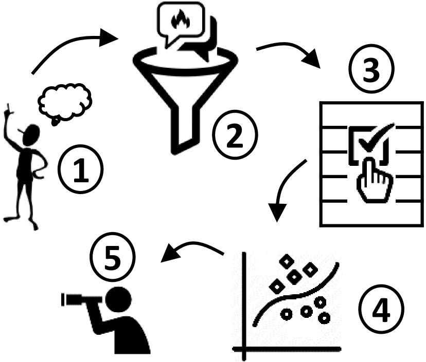
(a) Query-Based Tasks

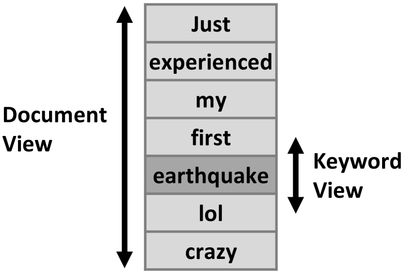
(b) Two Views in Our Model

Figure 1: 1(a)) Query-based tasks consist of five steps: 1) obtaining query phrases, 2) collecting the documents that contain the queries, 3) selecting a subset of the collected documents and labeling them, 4) training a classifier, and 5) predicting unseen documents. We use Active Learning to enhance the document selection in the third step and to consequently improve the classifier in the fourth step. 1(b)) We extract two views from documents: 1) a document view to encode the entire user posting, and 2) a keyword view to encode the context of the query phrase (earthquake). See Section 3.2 for more details.

A similar pipeline can be used in other tasks such as detecting suicide ideation Sawhney et al. (2020), monitoring press freedom Yousef et al. (2021), certain applications for hate speech detection An et al. (2021), certain applications for churn detection Amiri and Daume (2015), and general disease detection Karisani and Karisani (2020). In this study, we employ Active Learning Settles (2009) and aim to enhance the document sampling (Step 3) and the classification phase (Step 4) in this pipeline. See Figure 1(a) for an illustration.

Existing studies report various difficulties in mining social media data Imran et al. (2015); Stanovsky et al. (2017); Karisani et al. (2021). The costly construction of datasets is a challenge Karisani and Karisani (2021). To overcome this challenge, we use Active Learning which is known for reducing the amount of required data by intelligent sampling Settles (2009). Another issue is the typically short length of documents that, along small labeled data, can cause overfitting Karisani et al. (2021). To confront this challenge, we aim to use multi-view learning which is known for reducing the risk of overfitting Muslea et al. (2000); Nigam and Ghani (2000) by relying on models trained on different sets of features. See Figure 1(b) for an illustration of our algorithm for extracting the views. Another challenge is the noisy language of users in social media Xu et al. (2021). To address this obstacle, we use an active learning technique based on a committee of predictors. Ensemble learning is known for addressing noisy data by reducing variance Buhlmann and Yu (2002). Furthermore, and again related to noisy data, it is reported that social media users are highly inventive in using words Biddle et al. (2020). To tackle this challenge, we rely on the context of query phrases to identify word semantics Karisani et al. (2020); Bevilacqua et al. (2021).

Our study makes three contributions: 1) Existing active learning models for classifying social media data traditionally rely on single-view algorithms. In this paper, we propose the first multi-view active learning model in this domain. 2) We use pretrained contextual language models to extract our views. To efficiently use these views, we employ the Parzen-Rosenblatt window method Silverman (1986) and propose a novel query strategy by integrating the representativeness measure into multi-view Active Learning. 3) We use an algorithm based on the agreement between predictors to increase the resistance to social media noise. We empirically demonstrate that this step enhances the selection process in Active Learning.

We evaluate our model, which we term ROCAAL (Robust Context-Aware Active Learning), in four distinctly different Twitter tasks and demonstrate that it is either the top model or on a par with the best recent methods.

2 Related Work

The uncertainty-based sampling model is the most widely used active learning query strategy Lewis and Gale (1994); Attenberg and Provost (2011); Jedoui et al. (2019). In this model, the most informative document, i.e., the document that the base learner is uncertain about, is queried and added to the labeled pool. Ein-Dor et al. (2020) survey numerous methods and report that the performance of the classifiers based on pretrained language models can be enhanced by Active Learning, however, they also report that existing query strategies yield no significant gain over the uncertainty-based sampling model–measured by the prediction entropy.

Given the usually satisfactory performance of the uncertainty-based sampling model, the majority of successful applications of Active Learning in microblogging platforms rely on this model Burkhardt et al. (2020); Jiang et al. (2020); Zhao et al. (2020). The survey by Farinneya et al. (2021) confirms this claim, and also reports that language model pretraining can be an additional effective factor to address noisy social media data. Therefore, we follow their suggestion and use pretrained encoders in our model and all of the baselines.

Incorporating the diversity or the representativeness measures into the uncertainty-based query strategy is an active area of research Margatina et al. (2021); Zhang and Plank (2021); Yuan et al. (2020); Ru et al. (2020). While the uncertainty-based model, which is inherently a single-view model, has shown to be effective, it is well-known that multi-view models have a considerable potential Xu et al. (2013).

To our knowledge, there is no multi-view active learning model for social media data. In this article, we propose such a model by integrating the representativeness measure into multi-view Active Learning. Multi-view Active Learning Muslea et al. (2000); Ghani et al. (2003); Liao and Grishman (2011) constructs two views (or sets of features) from input data and trains a base learner on each view. Then each base learner is used to label the set of unlabeled data. The data points that are assigned to the opposite classes by the two base learners are detected–these data points are called contention points. One data point from this set is annotated and added to the labeled set. In the results and analysis section, we show that our model outperforms existing single-view models as well as the regular multi-view active learning model.

3 Proposed Model

We begin this section by explaining the problem statement, and then, we describe the approach to extract two views from documents. We continue by explaining the query strategy and the technique to tackle social media noise. Finally, we assemble the pieces and provide an overview of the model.

3.1 Problem Statement

We are given a small set of labeled user postings $L$, a large set of unlabeled user postings $U$, and the query phrase(s) $Q$, where $Q$ appears in all the documents of $L$ and $U$. We aim to to develop a selection mechanism to populate the set $L$ by the documents in $U$. Each document is annotated before being added to the set $L$. The objective is to reduce the error rate of the model trained on the set $L$ in labeling unseen documents.

We propose an active learning method to carry out the document selection step.

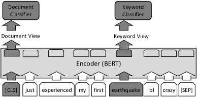
Figure 2: Pretrained multi-layer transformers as the encoder in our model. We employ these models–we used BERT in our experiments–to extract the document and the keyword representations. A hypothetical short and simple user posting is shown for demonstration. The token [CLS] in the BERT architecture represents the document encoding. To obtain the keyword representations, we extract the corresponding final pooling layers–see the experimental setup for the details.

3.2 Extracting Two Contextual Representations from Documents

The approach to construct two views from documents is inspired by the research on Word Sense Disambiguation (WSD) and their mainstream solutions the contextual word embeddings Bevilacqua et al. (2021). The neural contextual word embeddings are proven to encode the information required to effectively characterize word-level context Karisani et al. (2020). Thus, to extract two contextual representations from documents, we propose to extract one representation on the document level to capture global information about documents, and to extract another representation on the keyword level to capture the context that the query phrases were used in. To extract these representations we use pretrained transformers–e.g., BERT Devlin et al. (2019)–as the encoder to construct the document and keyword feature spaces. Since documents always contain at least one of the query phrases, then this task is always feasible.

We demonstrate this by outlining the task of detecting the true reports of earthquakes on Twitter, see Figure 2. Given the query words “quake” and “earthquake”, we may crawl the hypothetical tweet: “Just experienced my first earthquake lol crazy”. Given this tweet, we use the encoder to extract a feature vector on the document level which stores the overall information of the tweet. This corresponds to the tag [CLS] in the BERT architecture, as shown in Figure 2. Additionally, in the same manner we can extract another feature vector on the keyword level to capture the context of the search term, i.e., the vector representation of the search term in: “…my first earthquake lol…”.

Previous studies Balcan et al. (2005); Liao and Grishman (2011) have shown that correlated views are effective in multi-view learning. Thus, this approach is supported by empirical evidence. In the next section, we exploit these two views in an active learning framework.

3.3 Integrating Representativeness into Multi-View Active Learning

To develop our query strategy, we note that the ranking function, to select the best unlabeled documents, should be proportional to the confidence scores of the base learners in the two views. Because by definition a multi-view model is a contention reduction model, hence, for a document to be informative the classifier outputs must confidently point to the opposite directions. On the other hand, since we desire to incorporate document representativeness, the scores in each view should also represent the concentration of data points in the feature space.

To formally implement this idea, let $\vec{d}_{t}$ and $\vec{w}_{t}$ be the document and keyword level representations of the document $t$. The scoring function below follows our desired criteria outlined above:

$$\begin{split}score(t)=&P_{D}(\vec{d}_{t})\times Conf_{D}(\vec{d}_{t})~{}+~{}P_{W}(\vec{w}_{t})\times Conf_{W}(\vec{w}_{t}),\end{split}$$ (1)

where $Conf_{D}(\vec{d}_{t})$ and $Conf_{W}(\vec{w}_{t})$ are the confidence of the classifiers in the document level and in the keyword level views for labeling the example $t$. A classifier confidence is measured by the probability assigned to the output label Guo et al. (2017). A high probability means a high confidence. Therefore:

$$\begin{split}Conf_{D}(\vec{d}_{t})=\operatorname*{max}_{y}~{}~{}P_{\theta_{D}}(y|\vec{d}_{t}),\end{split}$$ (2)

and

$$\begin{split}Conf_{W}(\vec{w}_{t})=\operatorname*{max}_{y}~{}~{}P_{\theta_{W}}(y|\vec{w}_{t}),\end{split}$$ (3)

where the classifiers in the document and in the keyword level views are parameterized by $\theta_{D}$ and $\theta_{W}$ respectively. Note that in Equations 2 and 3, $P_{\theta_{\mathord{\color[rgb]{0.67,0.67,0.67}\bullet}}}(y|\mathord{\color[rgb]{0.67,0.67,0.67}\bullet})$ are real-valued probabilities, so are $Conf_{\mathord{\color[rgb]{0.67,0.67,0.67}\bullet}}(\mathord{\color[rgb]{0.67,0.67,0.67}\bullet})$. In Equation 1, $P_{D}(\vec{d}_{t})$ and $P_{W}(\vec{w}_{t})$ are the probabilities of the document $t$ belonging to the set of contention points in the document and in the keyword level views respectively. To obtain these quantities, we use the Parzen-Rosenblatt window method Silverman (1986). Therefore, we have:

$$\begin{split}P_{D}(\vec{d}_{t})=\frac{1}{n}~{}\sum_{i=1}^{n}~{}\frac{1}{(h_{1})^{b}}~{}\phi_{D}(\frac{\vec{d}_{t}-\vec{d}_{t_{i}}}{h_{1}}),\end{split}$$ (4)

and

$$\begin{split}P_{W}(\vec{w}_{t})=\frac{1}{n}~{}\sum_{i=1}^{n}~{}\frac{1}{(h_{2})^{b}}~{}\phi_{W}(\frac{\vec{w}_{t}-\vec{w}_{t_{i}}}{h_{2}}),\end{split}$$ (5)

where $n$ is the number of the contention points and $b$ is the number of dimensions–these quantities do not change across the views. $h_{1}$ and $h_{2}$ are called bandwidth hyper-parameters. $\phi_{D}(\mathord{\color[rgb]{0.67,0.67,0.67}\bullet})$ and $\phi_{W}(\mathord{\color[rgb]{0.67,0.67,0.67}\bullet})$ are the kernel functions. $\vec{d}_{t_{i}}$ and $\vec{w}_{t_{i}}$ are the representations of the contention document $t_{i}$ in the document and in the keyword level views respectively. Silverman (1986) discusses several kernel functions, including the triangular, Gaussian, and Epanechnikov kernels. The triangular kernel is the simplest one, which we use in our model. Thus we have:

$$\begin{split}\phi_{D}(\vec{a})=\left\{\begin{matrix}1-|\vec{a}|&\text{if}|\vec{a}|<h_{1}\\ 0&\text{otherwise},\\ \end{matrix}\right.\end{split}$$ (6)

and

$$\begin{split}\phi_{W}(\vec{a})=\left\{\begin{matrix}1-|\vec{a}|&\text{if}|\vec{a}|<h_{2}\\ 0&\text{otherwise},\\ \end{matrix}\right.\end{split}$$ (7)

where $|\vec{a}|$ is the vector norm.

Intuitively, our scoring function (Equation 1) assigns a higher score to the documents that are confidently assigned to the opposite classes in the two views (i.e., have a large distance from the decision boundaries in the two views), and are also close to the other set of contention points in each view. Figure 3 illustrates the principle. Each data point in the document representation space (the left panel) is associated to one data point in the keyword representation space (the right panel). The triangular data points are the set of contention documents, i.e., the documents that are assigned to the opposite classes by the classifiers in the two views. Based on our query strategy, the best candidate document has three properties: 1) It belongs to the set of contention data points, i.e., the triangular data points. 2) It is subject to the most disagreement between the two base learners. That is, it has a large distance from the decision boundaries, this is quantified by $Conf_{\mathord{\color[rgb]{0.67,0.67,0.67}\bullet}}(\mathord{\color[rgb]{0.67,0.67,0.67}\bullet})$ in Equation 1. 3) It is close to the other set of contention data points. This is quantified by $P_{\mathord{\color[rgb]{0.67,0.67,0.67}\bullet}}(\mathord{\color[rgb]{0.67,0.67,0.67}\bullet})$ in Equation 1.

The document that possesses the above three properties is indicated by a black triangle in Figure 3. We see that by querying this document, we can effectively infer the labels of the patch of red data points close to this document in both views.

There are two advantages in employing this scoring function. First, scaling the confidence of the base learners by the probability densities naturally aggregates the benefits of the contention reduction Abe and Mamitsuka (1998) and the density based Nguyen and Smeulders (2004) query strategies. Second, assuming that the points that are close to each other in the feature space are similar and are likely to have the same label, by promoting the documents that are close to the cluster of other contention points, we can effectively use the contextual information to resolve the disagreement over a set of similar documents. This is particularly the case when a candidate document and its adjacent points are projected into the same regions in both views.

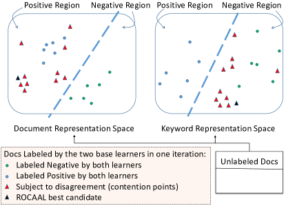
Figure 3: The document and keyword level views. ROCAAL queries the contention point which is closest to the set of other contention points and also has a large distance from the decision boundaries in the two views (the black triangle). Figure best viewed in color.

3.4 Enhancing Resistance to Noise

As pointed out by Farzindar and Inkpen (2020), the documents in social media–particularly on the Twitter website–are highly noisy. They tend to be short, and are packed with inventive lexicons. For instance, in our early example of extracting the reports of earthquakes, a document may be added to the set of contention points and selected for annotation by accident due its noisy content, e.g., the existence of irregular or figurative language. However, selecting another document for annotation might be a better choice to have a diverse and representative training set. If we assume relatively uninformative documents are noise–which due to their unique characteristics may receive a high score by Equation 1–then we may be able to dampen their effect by variance reduction algorithms.

To address this issue we propose to employ multiple predictors. Bagging is empirically shown to reduce model variance Buhlmann and Yu (2002). In the discussed example, bagging can influence the score of the mentioned document, either through affecting the distribution of the contention documents, or reducing the disagreement rate between the two base learners. While it is well-known that bagging is effective for model prediction Gareth et al. (2013), we haven’t found any recent study to further investigate the utility of bagging for decision making in Active Learning Abe and Mamitsuka (1998). In the analysis section, we empirically demonstrate that our proposed technique (see below) for bagging not only improves model prediction, but also enhances the decision making by promoting better candidate documents. We also particularly show that this step enables our model to outperform the baselines that use the regular bagging and also those that use multiple classifiers.

We use this technique as follows: In each iteration, we sample multiple subsets of documents from the set of labeled data. On each subset, we train a pair of base learners as described in Section 3.2. For each pair of base learners, we use the model described in Section 3.3 to assign a score to all the unlabeled documents. Finally, the ultimate ranking list is constructed by aggregating the scores of the unlabeled data across the models.

Our technique is different from the regular bagging model Abe and Mamitsuka (1998). In the regular bagging model, one estimator is trained on each subset of data, and the best candidate data point is the data point which is subject to the most disagreement among the estimators. In our model, the candidate data points, for each subset, are the data points that are assigned to the opposite classes by the base learners. Then, each pair of base learners vote for the candidate data points, and the best candidate data point is the one that is subject to the most agreement among all the pairs.

Algorithm 1 Single Iteration of ROCAAL 

1:procedure ROCAAL 

2:   Given:    

3:     $L:\text{Set of labeled documents}$

4:     $U:\text{Set of unlabeled documents}$

5:     $T:\text{Set of test documents}$

6:     $K:\text{Number of estimators for bagging}$    

7:   Return:    

8:     Labeled set of test documents & updated training set    

9:   Execute:

10:   Define $S$ as 1-d array // to store the sub-samples

11:   Define $BL$ as 2-d array // to store the base learners

12:   Define $DS$ as 2-d array // to store the Parzen models

13:   Define $C$ as 1-d array // to store the contention docs

14:   Define $Conf$ as 2-d array // to store confidence scores

15:   Define $P$ as 2-d array // to store the probability values    

16:     for $i\leftarrow 1$ to $K$ do

17:       Sample a subset of L and store in $S[i]$

18:       Train two base learners on the two views of $S[i]$ and store in $BL[i][0]$ and $BL[i][1]$

19:       Use $BL[i][0]$ and $BL[i][1]$ to label the set $U$

20:       Store the contention documents in $C[i]$, and their prediction confidences in $Conf[i][0]$ and $Conf[i][1]$

21:       Train two Parzen models on the two views of $C[i]$ and store them in $DS[i][0]$ and $DS[i][1]$

22:       Use $DS[i][0]$ and $DS[i][1]$ to calculate the probability mass values for all the documents in $C[i]$ and store them in $P[i][0]$ and $P[i][1]$      

23:     Plug the arrays $Conf$ and $P$ into Equation (1) to calculate the aggregated score for documents in $C$

24:     Rank all the documents in $C$ based on their score, and store the top one in the new variable $W$

25:     Query the label of $W$ // Active Learning Query

26:     Add $W$ to $L$ and to every $S[\mathord{\color[rgb]{0.67,0.67,0.67}\bullet}]$ in $S$

27:     Retrain the base learners in $BL[\mathord{\color[rgb]{0.67,0.67,0.67}\bullet}]$ on their corresponding updated sets in $S$

28:     for $doc$ in $T$ do

29:       $PCount\leftarrow 0$

30:       for $cls\_pair$ in $BL$ do

31:         Use the two classifiers in $cls\_pair$ to label the document $doc$ and aggregate the outputs, if the final label is positive then increment $PCount$        

32:       If $(PCount\geq K/2)$ then $doc$ is positive, otherwise it is negative      

33:     $\text{Return }T,L$    

3.5 Overview of Algorithm

Algorithm 1 summarizes one iteration of ROCAAL ​. Here we leave out the implementation details and only mention the primary steps.

Lines 16-27 describe the training procedure, and Lines 28-32 describe the labeling procedure. The training stage begins by sampling from the set of labeled documents; then two base learners are trained on the two views of the sampled set. The two base learners are used to label the set of unlabeled documents. The contention documents are detected, and in each view one Parzen-Rosenblatt window method is trained. The two models are used to approximate the probability mass values of every contention document. These steps are repeated for each sub-sample. To rank the set of unlabeled documents, the prediction confidences and probability mass values are used in Equation 1 to score all of the contention documents. One document with the highest score is selected and queried to be added to the labeled set and all of the sampled sets–Line 25 and Line 26. Finally, all of the base learners are re-trained on the updated sampled sets. In the labeling stage, each pair of the base learners is used to label the test documents–Line 31. To predict the final label, a majority voting algorithm is used–Line 32.

4 Experimental Setup

In this section we discuss the datasets, the baselines, and the implementation details. See Appendix A for more details on the used datasets.

4.1 Datasets

Social media is a multi-million dollar industry. It can be weaponized to target the basis of democracy or it can be a powerful tool for humanitarian aid. However, as stated in Section 1, mining this resource is challenging, which is the motivation for our research. To extensively evaluate our model we use four distinctly different and publicly available Twitter datasets.

Detecting reports of product consumption. We use the dataset introduced by Weissenbacher et al. (2019) for an ACL shared task. A document in this dataset is positive if it reports consuming a product. We use the product references to construct the keyword view.

Detecting rumours. We include the dataset introduced by Kochkina et al. (2018), the revision prepared by Wright and Augenstein (2020). In this dataset a document is positive if it spreads a rumour. We use the rumour phrases to construct the keyword view.

Detecting reports of medical drug side-effects. We use the dataset introduced and expanded by Magge et al. (2021). This dataset has been used for several consecutive years in various NLP shared tasks including NAACL 2021. A document in this dataset is positive if it reports the side-effects of a drug. We use the drug references to construct the keyword view.

Detecting reports of observations. We include the dataset introduced by Zahra et al. (2020). In this dataset a document is positive if it reports direct experience with a natural crisis, e.g., an earthquake. We use the crisis phrases to construct the keyword view.

Table 1 reports the size of each dataset, along the number of positive and negative documents in each one. We see that the rumour dataset is the smallest one and the ADR dataset is the largest one, with ADR being the most imbalanced benchmark.

Dataset	Set	# Doc	# Neg	# Pos
Product	Train	4,503	3,104	1,399
	Test	2,114	1,648	466
	Total	6,617	4,752	1,865
Rumour	Train	4,001	2,641	1,360
	Test	1,801	1,189	612
	Total	5,802	3,830	1,972
ADR	Train	20,624	18,659	1,965
	Test	4,992	4,581	411
	Total	25,616	23,240	2,376
Observation	Train	7,998	5,694	2,304
	Test	6,001	4,911	1,090
	Total	13,999	10,605	3,394

Table 1: The size and the class distribution of the datasets.

4.2 Baselines

We compare our model with a wide range of baselines, including those that use bagging and use multiple classifiers. All the models (the baselines and our model) use pretrained BERT as the encoder–see the next section for details.

random: This baseline is without Active Learning. In each iteration, we randomly select one document from the set of unlabeled data and add to the labeled set. Then, retrain the base learner.

uncertainty: It is the uncertainty-based model Settles (2009). The output entropy of the base learner was used as the selection criterion.

qbc: It is a query-by-committee model constructed via bagging with 20 classifiers and 60% sampling ratio Settles (2009). In this model, the document with the highest rate of disagreement between the classifiers is selected for annotation.

lal: It is an ensemble with 20 predictors proposed by Konyushkova et al. (2017). This model is a meta-learning algorithm. The authors argue that instead of manually crafting query strategies, a model should be able to learn the query strategy. They propose to use a regressor that learns the best strategy in the given task. The model estimates the expected error of every data point, then queries the data point that maximizes the error reduction.

caral: It is proposed by Zhang and Plank (2021). In this model, the informativeness of data points is defined by the variation in their consecutive predictions during the training of the classifier. The model relies on data maps Swayamdipta et al. (2020), which uses these predictions to categorize data points into easy, ambiguous, and hard. The authors argue that the data points on the boundary of ambiguous and hard categories are the best candidates and contain the highest diversity.

cal: It is proposed by Margatina et al. (2021). In this model, the diversity and informativeness are combined by choosing the data point that is most similar to its neighbours, but is assigned to the opposite class labels. To contrast two data points, the authors use the Kullback-Leibler divergence Kullback and Leibler (1951) between the classifier predictions.

4.3 Implementation Details

We adopt the standard practice in the active learning literature to carry out the experiments Settles (2009); Lowell et al. (2019). In the cold start state, we randomly sample 50 labeled documents, and assume that the rest of the labeled data is unlabeled. This is a standard practice in the literature Settles (2009); active learning methods enhance the quality of selected data as the algorithm proceeds Lowell et al. (2019); Siddhant and Lipton (2018). We report performance in the test set as the training set is augmented with new labeled documents. Following the argument made by Mccreadie et al. (2019) about imbalanced datasets, to consider the classifier quality (Precision) and coverage (Recall) we report the F1 in the minority set. We repeat all the experiments 5 times with different random seeds and report the average of the runs.

We use pretrained BERT base Devlin et al. (2019); Wolf et al. (2019) as the encoder in all the models. Note that this makes any improvement difficult, because the pretrained transformers are already robust in data scarce settings Devlin et al. (2019), and any improvement should be additive to these baselines. The size of the vectors in BERT is 768 and as suggested by Devlin et al. (2019) we use the average of the last 4 layers to create the vectors–they suggest this based on empirical evidence. We use a one-layer fully connected network as the classifier in all the models. Thus, all the models use an identical network and an identical pretraining/fine-tuning procedure, therefore, their comparison is completely fair.

To implement our model, when multiple mentions of the same keyword are included in the same document, the representation of the first one is used. If the queries consist of multi-word phrases, for simplicity, we use the first word in the sequence as the keyword representation. However, an alternative is to replace the phrases with a synthesized token Karisani et al. (2020); Shi and Lin (2019). In Equations 4 and 5, the variable $b$ is the size of the BERT vectors, that is 768. There are multiple ways to set the bandwidths $h_{1}$ and $h_{2}$ in the Parzen-Rosenblat window method Heidenreich et al. (2013). We set these quantities to the average distance of the data points in the document and in the keyword level views respectively (30 and 45), which is independent of labeled data. In our bagging algorithm, we use 10 estimators with 60% sampling ratio.

5 Results and Analysis

In this section we report the results and then we provide an empirical analysis.

5.1 Results

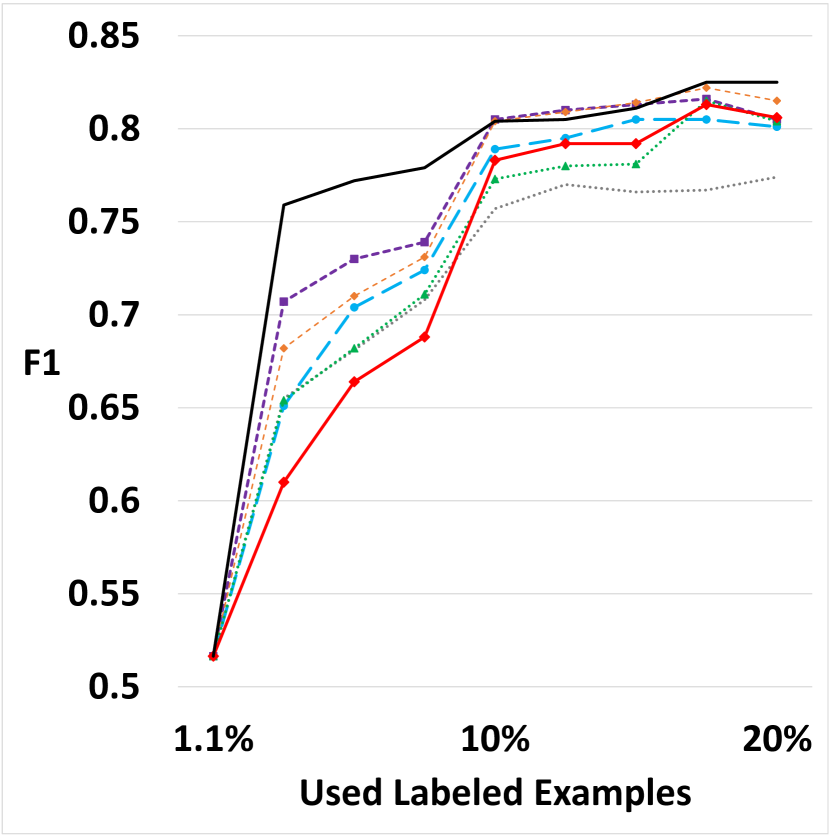
(a) Product 

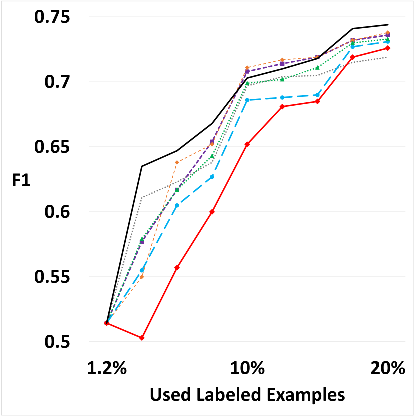
(b) Rumour 

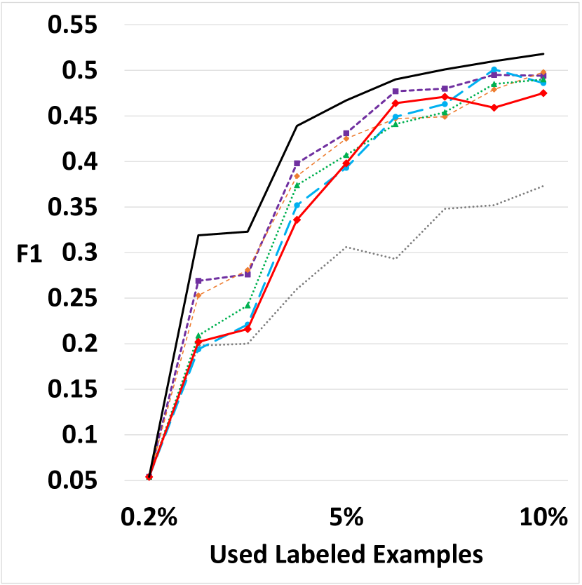
(c) ADR 

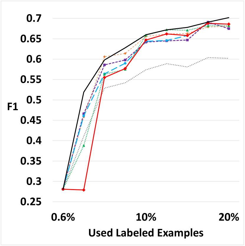
(d) Observation 

Figure 4: Learning curves of the models in the four datasets. Note that the horizontal axis units are 5 percent absolute value. We see that as more labeled data is used all the models almost converge Attenberg and Provost (2011). Figure best viewed in color.

Figure 4 reports the performance of our model compared to that of the baselines in all the datasets. The results confirm that–except in a few cases–all the models outperform random baseline, confirming that Active Learning is effective in these tasks. The experiments also show that uncertainty model is performing very well, confirming the consistency of this model which is discussed in Section 2 and is also reported in other studies Attenberg and Provost (2011); Ein-Dor et al. (2020). Finally, the results signify that our model ROCAAL consistently improves over the baselines. During the early iterations, our model exploits two views to issue the queries, whereas the other models rely on one view. This is significant, since in real-world scenarios the set of labeled data points is small and costly to obtain. As more training data becomes available and the pool of unlabeled data shrinks, the models converge Attenberg and Provost (2011). Nonetheless, our model still maintains a noticeable superiority. Table 2 reports the final performance of the models.

	F1 in datasets
Method	Product	Rumour	ADR	Observation
random	0.774$\pm$0.01	0.719$\pm$0.02	0.373$\pm$0.06	0.602$\pm$0.02
uncertainty	0.805$\pm$0.01	0.736$\pm$0.01	0.494$\pm$0.02	0.675$\pm$0.01
qbc	0.815$\pm$0.01	0.738$\pm$0.02	0.498$\pm$0.02	0.681$\pm$0.01
lal	0.801$\pm$0.01	0.731$\pm$0.00	0.486$\pm$0.03	0.686$\pm$0.02
caral	0.804$\pm$0.00	0.733$\pm$0.01	0.490$\pm$0.01	0.682$\pm$0.01
cal	0.806$\pm$0.01	0.726$\pm$0.02	0.475$\pm$0.03	0.686$\pm$0.02
ROCAAL	0.825$\pm$0.01	0.744$\pm$0.01	0.518$\pm$0.02	0.702$\pm$0.01

Table 2: Final F1 measure of our model compared to that of the baselines in all the datasets.

5.2 Empirical Analysis

We begin this section by reporting an ablation study on the efficacy of the individual views. Then, we report a second ablation study on the efficacy of each module in our model (i.e., our query strategy and our variance reduction technique) and also compare with the regular multi-view active learning. Then we evaluate the impact of our variance reduction technique on the decision making in active learning. Finally, we discuss the resource complexity and the hyper-parameter sensitivity of our model.

Method	F1	Precision	Recall
Keyword view	0.452	0.528	0.398
Document view	0.494	0.639	0.406
ROCAAL	0.518	0.606	0.454

Table 3: The performance in the document level and keyword level views compared to ROCAAL .

To demonstrate the efficacy of the views proposed in Section 3.2, we report an ablation study by leaving out each view and training a model on the remaining view. Table 3 reports the results. We see that both views have a contribution. We particularly see that the model trained on the document view has a much better performance. This experiment and the next ones require to run a model numerous times. We carried them out in ADR dataset.

We report a second ablation study on the role of our novel active learning query strategy (Section 3.3) and on the role of our technique for tackling the effect of noise in informal social media documents using a variance reduction method (Section 3.4). In each case, the new model is obtained by leaving out one module and evaluating the remaining module. Table 4 reports the results of this experiment. We see that both modules have noticeable influence. In this experiment, we also compare our model with the regular multi-view active learning. This model is obtained by deactivating both modules. We see that it is markedly outperformed.

To demonstrate that our variance reduction technique (Section 3.4) specifically improves the candidate selection in Active Learning we need to disentangle the impact of this algorithm from the prediction. To this end, we run two variants of our model. In the first variant we use multiple predictors in the query strategy to select the best candidate document, then we randomly select one pair of the predictors for labeling. In the second variant we use one pair of predictors in the query strategy, then we create a pool of multiple predictors for labeling. Table 5 reports the results of this experiment. We observe that our algorithm improves both the query selection and the prediction (in terms of F1). We see that there is an increase in the precision when we use multiple estimators in the query strategy.

In terms of runtime, our model takes about 10 seconds on average to make one query in ADR dataset–using a system with a 16-core processor and an NVIDIA Titan RTX GPU. One particularly interesting quality of our model is the absence of critical hyper-parameters to tune. Excluding the hyper-parameters of the base learners, which is shared between all the baselines, in our experiments ROCAAL was not sensitive to other hyper-parameters. Figure 5 reports the performance of our model at varying values of the bandwidths $h1$ and $h2$. We set these quantities to 30 and 45 based on the average distance of the data points in the document and the keyword level views, which is independent of the labeled data. We see that the performance reaches a plateau after a certain threshold. We used {10,15,20} as the number of estimators and used {0.6,0.7,0.8} as the sampling ratio in bagging, but didn’t observe a noticeable sensitivity.

In summary, we used four publicly available datasets in the experiments, and also included multiple state-of-the-art and traditional baselines, and showed that our model consistently outperforms them. We also reported detailed experiments and empirically analyzed our model from multiple aspects.

Method	F1	Precision	Recall
Regular multi-view	0.496	0.618	0.415
ROCAAL (only varian. reduct.)	0.507	0.613	0.433
ROCAAL (only query strategy)	0.508	0.650	0.416
ROCAAL	0.518	0.606	0.454

Table 4: Ablation study on the efficacy of the query strategy and the variance reduction technique. We see that both steps are equally contributing.

Method	F1	Precision	Recall
Bagging for selection	0.512	0.650	0.423
Bagging for prediction	0.513	0.638	0.430
ROCAAL	0.518	0.606	0.454

Table 5: The impact of bagging on the query selection and on the prediction stages.

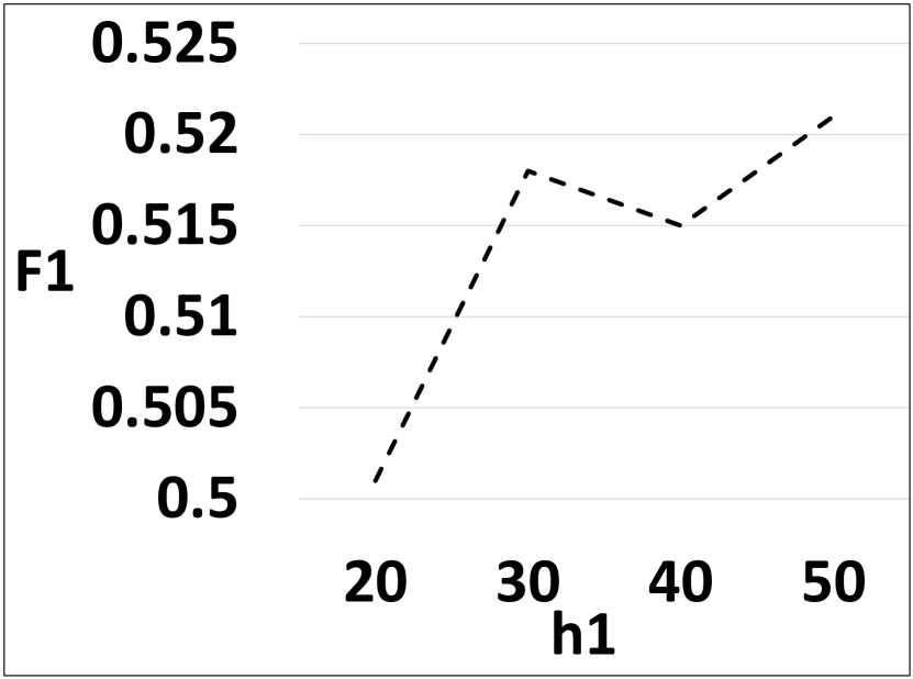
(a) F1 vs h1

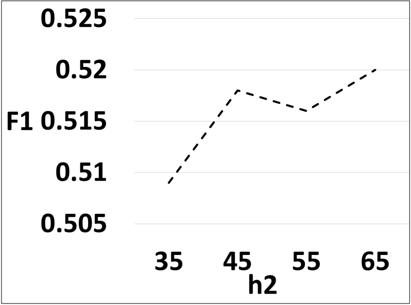
(b) F1 vs h2

Figure 5: The sensitivity of ROCAAL to the hyper-parameters.

Certain tasks such as general event detection use templates instead of query phrases. Linguistic templates, or extraction patterns Riloff and Jones (1999), cannot be incorporated into our model as is. Future work may explore this direction. Another interesting direction is investigating the efficacy of our model on the platforms with longer documents, e.g., on Amazon or on IMDB. The longer length of documents and the higher occurrence of query phrases can pose exciting research challenges.

6 Conclusions

In this paper, we proposed an active learning model for social media tasks tailored for query phrases. We employed an algorithm to derive two views from documents, then, we proposed a new multi-view query strategy to aggregate the representativeness and the contention reduction measures. Finally, we proposed an algorithm based on the agreement between multiple predictors to tackle noisy content. Through an extensive set of experiments in four public datasets we showed that our model outperforms existing baselines. We also reported two ablation studies and extensively analyzed our model.

Limitations

Limitations in methodology. We have proposed an active learning model for a category of tasks called Query-Based problems. We argued in the paper that this category covers a large and diverse set of scenarios. Nonetheless, this category is not a complete set by any means. There exist tasks that fall outside this set and are not query-based, e.g., general offensive language detection and certain event detection tasks. Our model, as is, cannot be used to perform such tasks. To address this limitation our model should be able to incorporate extraction patterns. This enables our model to handle tasks that use lexical templates, such as some event detection problems. We may explore this direction in the future.

Limitations in experiments. The efficacy of our model depends on the expressiveness of the underlying views extracted from documents. These views are based on contextual word embeddings. Using four English datasets, we experimentally showed that the views extracted by the pretrained BERT are sufficient for this. One can ask whether such views can be extracted from non-English language models. Our paper focuses on English tasks only, and has not explored other languages.

Failure mode and potential misuse. If our model is used as described in this paper, we expect that it enhances model performance. We used four datasets across various domains to reduce the risk of any bias. Nonetheless, every domain has a specific data distribution and this can affect the efficacy of active learning algorithms Attenberg and Provost (2011).

Privacy. All the datasets used in our paper are public and have been recently used in NLP venues. The publishers of these datasets have targeted important applications that can benefit the society. Nonetheless, if one decides to use our model for processing a new task, they should follow the corresponding terms of service. Most importantly, they should not collect any personal information about users, and should not use our model in sensitive tasks that violate user privacy.

Costs. Our model aims at reducing the cost of development. Nonetheless, to design our model and to run the baselines, we ran the experiments several dozens of times using a system with a 16-core processor and eight NVIDIA Titan RTX GPUs. Note that in a deployment environment, there is no need to consume such a resource. Because our model can be used as is.

Dataset	Document Length (Mean)	Document Length (Median)	Total # of Unique Tokens
Product	15.7	15	14,821
Rumour	16.1	16	13,091
ADR	16.4	17	43,413
Observation	14.7	15	28,398

Table 6: The average and the median of the documents in the datasets (in number of tokens), the third column shows the total number of unique tokens in each dataset. To tokenize the documents we used the parser developed by Kong et al. (2014). The numbers are without punctuation marks.

Dataset	# of Used Queries	Query Length (Mean)	# of Queries in Document (Mean)
Product	2	1	1.2
Rumour	6	2	1
ADR	493	1	1.3
Observation	4	1	0.95

Table 7: The total number of used queries to collect the datasets, the average length of used queries (in number of words), and the average number of queries appearing in a document.

Appendix A Data Analysis

In this section, we investigate two relevant aspects of the datasets used in the experiments. Table 6 reports the average length of the documents in each dataset. We see that the ADR dataset, which is also the largest one, has the largest set of unique tokens.

Table 7 reports the characteristics of the queries used to collect the datasets. We see that the query set of ADR is extremely large. Note that the average number of queries in a document in the Observation dataset is less than 1. This is despite the fact that the creators of the dataset report that they have collected the data using keywords Zahra et al. (2020). As a patch for such cases, we used the vector representation of the document view as the vector representation of the keyword view–essentially ignoring the missing keywords.

References

- Abe and Mamitsuka (1998) Naoki Abe and Hiroshi Mamitsuka. 1998. Query learning strategies using boosting and bagging. In Proc of the 5th ICML, pages 1–9.
- Abulaish et al. (2020) Muhammad Abulaish, Ashraf Kamal, and Mohammed J. Zaki. 2020. A survey of figurative language and its computational detection in online social networks. ACM Transactions on the Web, 14(1):3:1–3:52.
- Amiri and Daume (2015) Hadi Amiri and Hal Daume. 2015. Target-dependent churn classification in microblogs. In Proceedings of the Twenty-Ninth AAAI Conference on Artificial Intelligence, January 25-30, 2015, Austin, Texas, USA, pages 2361–2367. AAAI Press.
- An et al. (2021) Jisun An, Haewoon Kwak, Claire Seungeun Lee, Bogang Jun, and Yong-Yeol Ahn. 2021. Predicting anti-asian hateful users on twitter during COVID-19. In Findings of the Association for Computational Linguistics: EMNLP 2021, Virtual Event / Punta Cana, Dominican Republic, 16-20 November, 2021, pages 4655–4666. Association for Computational Linguistics.
- Attenberg and Provost (2011) Josh Attenberg and Foster Provost. 2011. Inactive learning?: Difficulties employing active learning in practice. KDD Exp. News., 12:36–41.
- Balcan et al. (2005) Maria-Florina Balcan, Avrim Blum, and Ke Yang. 2005. Co-training and expansion: Towards bridging theory and practice. In NIPS, pages 89–96.
- Bevilacqua et al. (2021) Michele Bevilacqua, Tommaso Pasini, Alessandro Raganato, and Roberto Navigli. 2021. Recent trends in word sense disambiguation: A survey. In Proceedings of the Thirtieth International Joint Conference on Artificial Intelligence, IJCAI 2021, Virtual Event / Montreal, Canada, 19-27 August 2021, pages 4330–4338. ijcai.org.
- Biddle et al. (2020) Rhys Biddle, Aditya Joshi, Shaowu Liu, Cecile Paris, and Guandong Xu. 2020. Leveraging sentiment distributions to distinguish figurative from literal health reports on twitter. In Proceedings of The Web Conference 2020, WWW ’20, page 1217–1227, New York, NY, USA. Association for Computing Machinery.
- Buhlmann and Yu (2002) Peter Buhlmann and Bin Yu. 2002. Analyzing bagging. Ann. Statist., 30(4):927–961.
- Burkhardt et al. (2020) Sophie Burkhardt, Julia Siekiera, Josua Glodde, Miguel A Andrade-Navarro, and Stefan Kramer. 2020. Towards identifying drug side effects from social media using active learning and crowd sourcing. In Pacific Symposium of Biocomputing (PSB), pages 319–330.
- Chapelle et al. (2003) Olivier Chapelle, Jason Weston, and Bernhard Schölkopf. 2003. Cluster kernels for semi-supervised learning. In NIPS 15, pages 601–608. MIT Press.
- Devlin et al. (2019) Jacob Devlin, Ming-Wei Chang, Kenton Lee, and Kristina Toutanova. 2019. BERT: Pre-training of deep bidirectional transformers for language understanding. In Proc of the 2019 NAACL, pages 4171–4186.
- Efron (2011) Miles Efron. 2011. Information search and retrieval in microblogs. Journal of the American Society for Information Science and Technology (JASIST), 62(6):996–1008.
- Ein-Dor et al. (2020) Liat Ein-Dor, Alon Halfon, Ariel Gera, Eyal Shnarch, Lena Dankin, Leshem Choshen, Marina Danilevsky, Ranit Aharonov, Yoav Katz, and Noam Slonim. 2020. Active learning for BERT: an empirical study. In Proceedings of the 2020 Conference on Empirical Methods in Natural Language Processing, EMNLP 2020, Online, November 16-20, 2020, pages 7949–7962.
- Farinneya et al. (2021) Parsa Farinneya, Mohammad Mahdi Abdollah Pour, Sardar Hamidian, and Mona T. Diab. 2021. Active learning for rumor identification on social media. In Findings of the Association for Computational Linguistics: EMNLP 2021, Virtual Event / Punta Cana, Dominican Republic, 16-20 November, 2021, pages 4556–4565.
- Farzindar and Inkpen (2020) Anna Atefeh Farzindar and Diana Inkpen. 2020. Natural Language Processing for Social Media, Third Edition. Synthesis Lectures on Human Language Technologies. Morgan & Claypool Publishers.
- Gareth et al. (2013) James Gareth, Witten Daniela, Hastie Trevor, and Tibshirani Robert. 2013. An introduction to statistical learning: with applications in R. Spinger.
- Ghani et al. (2003) Rayid Ghani, Rosie Jones, Tom Mitchell, and Ellen Riloff. 2003. Active learning for information extraction with multiple view feature sets. In Proc of the 20th ICML, pages 26–34.
- Guo et al. (2017) Chuan Guo, Geoff Pleiss, Yu Sun, and Kilian Q. Weinberger. 2017. On calibration of modern neural networks. In Proceedings of the 34th International Conference on Machine Learning, ICML 2017, Sydney, NSW, Australia, 6-11 August 2017, volume 70 of Proceedings of Machine Learning Research, pages 1321–1330.
- Heidenreich et al. (2013) Nils-Bastian Heidenreich, Anja Schindler, and Stefan Sperlich. 2013. Bandwidth selection for kernel density estimation: a review of fully automatic selectors. AStA Advances in Statistical Analysis, 97(4):403–433.
- Imran et al. (2015) Muhammad Imran, Carlos Castillo, Fernando Diaz, and Sarah Vieweg. 2015. Processing social media messages in mass emergency: A survey. ACM Comput. Surv., 47(4):67:1–67:38.
- Jedoui et al. (2019) Khaled Jedoui, Ranjay Krishna, Michael Bernstein, and Li Fei-Fei. 2019. Deep bayesian active learning for multiple correct outputs. arXiv preprint arXiv:1912.01119.
- Jiang et al. (2020) Zhuoren Jiang, Zhe Gao, Yu Duan, Yangyang Kang, Changlong Sun, Qiong Zhang, and Xiaozhong Liu. 2020. Camouflaged Chinese spam content detection with semi-supervised generative active learning. In Proceedings of the 58th Annual Meeting of the Association for Computational Linguistics, pages 3080–3085, Online. Association for Computational Linguistics.
- Karisani and Karisani (2020) Negin Karisani and Payam Karisani. 2020. Mining coronavirus (covid-19) posts in social media. arXiv preprint arXiv:2004.06778.
- Karisani and Agichtein (2018) Payam Karisani and Eugene Agichtein. 2018. Did you just have a heart attack?: Towards robust detection of personal health mentions in social media. In Proc of the 2018 WWW, pages 137–146.
- Karisani et al. (2020) Payam Karisani, Eugene Agichtein, and Joyce Ho. 2020. Domain-guided task decomposition with self-training for detecting personal events in social media. In Proceedings of The Web Conference 2020, WWW ’20, page 2411–2420, New York, NY, USA. Association for Computing Machinery.
- Karisani et al. (2021) Payam Karisani, Jinho D. Choi, and Li Xiong. 2021. View distillation with unlabeled data for extracting adverse drug effects from user-generated data.
- Karisani and Karisani (2021) Payam Karisani and Negin Karisani. 2021. Semi-supervised text classification via self-pretraining. In Proceedings of the 14th ACM International Conference on Web Search and Data Mining, WSDM ’21, page 40–48. Association for Computing Machinery.
- Kochkina et al. (2018) Elena Kochkina, Maria Liakata, and Arkaitz Zubiaga. 2018. All-in-one: Multi-task learning for rumour verification. In Proceedings of the 27th International Conference on Computational Linguistics, COLING 2018, Santa Fe, New Mexico, USA, August 20-26, 2018, pages 3402–3413. Association for Computational Linguistics.
- Kong et al. (2014) Lingpeng Kong, Nathan Schneider, Swabha Swayamdipta, Archna Bhatia, Chris Dyer, and Noah A. Smith. 2014. A dependency parser for tweets. In Proceedings of the 2014 Conference on Empirical Methods in Natural Language Processing, (EMNLP 2014), pages 1001–1012.
- Konyushkova et al. (2017) Ksenia Konyushkova, Raphael Sznitman, and Pascal Fua. 2017. Learning active learning from data. In Advances in Neural Information Processing Systems (NIPS) 30, pages 4225–4235. Curran Associates, Inc.
- Kullback and Leibler (1951) Solomon Kullback and Richard A Leibler. 1951. On information and sufficiency. The annals of mathematical statistics, 22(1):79–86.
- Lewis and Gale (1994) David D. Lewis and William A. Gale. 1994. A sequential algorithm for training text classifiers. In Proc of the 17th SIGIR, pages 3–12.
- Liao and Grishman (2011) Shasha Liao and Ralph Grishman. 2011. Using prediction from sentential scope to build a pseudo co-testing learner for event extraction. In Proc of 5th IJCNLP, pages 714–722.
- Lowell et al. (2019) David Lowell, Zachary C. Lipton, and Byron C. Wallace. 2019. Practical obstacles to deploying active learning. In Proc of the 2019 EMNLP, pages 21–30.
- Magge et al. (2021) Arjun Magge, Ari Klein, Antonio Miranda-Escalada, Mohammed Ali Al-Garadi, Ilseyar Alimova, Zulfat Miftahutdinov, Eulalia Farre, Salvador Lima López, Ivan Flores, Karen O’Connor, Davy Weissenbacher, Elena Tutubalina, Abeed Sarker, Juan Banda, Martin Krallinger, and Graciela Gonzalez-Hernandez. 2021. Overview of the sixth social media mining for health applications (#SMM4H) shared tasks at NAACL 2021. In Proceedings of the Sixth Social Media Mining for Health (#SMM4H) Workshop and Shared Task, Mexico City, Mexico. Association for Computational Linguistics.
- Margatina et al. (2021) Katerina Margatina, Giorgos Vernikos, Loïc Barrault, and Nikolaos Aletras. 2021. Active learning by acquiring contrastive examples. In Proceedings of the 2021 Conference on Empirical Methods in Natural Language Processing, EMNLP 2021, Virtual Event / Punta Cana, Dominican Republic, 7-11 November, 2021, pages 650–663.
- Mccreadie et al. (2019) R. Mccreadie, C. Buntain, and I. Soboroff. 2019. Trec incident streams: Actionable information on social media. In Proc of the 16th ISCRAM.
- Muslea et al. (2000) Ion Muslea, Steven Minton, and Craig A. Knoblock. 2000. Selective sampling with redundant views. In Proc of the Seventeenth National Conference on Artificial Intelligence and Twelfth Conference on Innovative Applications of Artificial Intelligence, pages 621–626. AAAI Press.
- Nguyen and Smeulders (2004) Hieu T. Nguyen and Arnold Smeulders. 2004. Active learning using pre-clustering. In Proc of the Twenty-first International Conference on Machine Learning, ICML ’04, pages 79–.
- Nigam and Ghani (2000) Kamal Nigam and Rayid Ghani. 2000. Analyzing the effectiveness and applicability of co-training. In Proc of the 2000 ACM CIKM International Conference on Information and Knowledge Management, McLean, VA, USA, November 6-11, 2000, pages 86–93.
- Riloff and Jones (1999) Ellen Riloff and Rosie Jones. 1999. Learning dictionaries for information extraction by multi-level bootstrapping. In Proceedings of the Sixteenth National Conference on Artificial Intelligence and Eleventh Conference on Innovative Applications of Artificial Intelligence, July 18-22, 1999, Orlando, Florida, USA, pages 474–479. AAAI Press / The MIT Press.
- Ru et al. (2020) Dongyu Ru, Jiangtao Feng, Lin Qiu, Hao Zhou, Mingxuan Wang, Weinan Zhang, Yong Yu, and Lei Li. 2020. Active sentence learning by adversarial uncertainty sampling in discrete space. In Findings of the Association for Computational Linguistics: EMNLP 2020, Online Event, 16-20 November 2020, volume EMNLP 2020 of Findings of ACL, pages 4908–4917.
- Sawhney et al. (2020) Ramit Sawhney, Harshit Joshi, Saumya Gandhi, and Rajiv Ratn Shah. 2020. A time-aware transformer based model for suicide ideation detection on social media. In Proceedings of the 2020 Conference on Empirical Methods in Natural Language Processing, EMNLP 2020, Online, November 16-20, 2020, pages 7685–7697. Association for Computational Linguistics.
- Settles (2009) Burr Settles. 2009. Active learning literature survey. Computer Sciences Technical Report 1648, University of Wisconsin–Madison.
- Shi and Lin (2019) Peng Shi and Jimmy Lin. 2019. Simple bert models for extraction and semantic role labeling. arXiv preprint arXiv:1904.05255.
- Siddhant and Lipton (2018) Aditya Siddhant and Zachary C. Lipton. 2018. Deep bayesian active learning for natural language processing: Results of a large-scale empirical study. In Proceedings of the 2018 Conference on Empirical Methods in Natural Language Processing, Brussels, Belgium, October 31 - November 4, 2018, pages 2904–2909. Association for Computational Linguistics.
- Silverman (1986) Bernard W Silverman. 1986. Density estimation for statistics and data analysis, volume 26. CRC press.
- Stanovsky et al. (2017) Gabriel Stanovsky, Daniel Gruhl, and P Mendes. 2017. Recognizing mentions of adverse drug reaction in social media using knowledge-infused recurrent models. In Proc of the 15th EACL, pages 142–151.
- Sun (2013) Shiliang Sun. 2013. A survey of multi-view machine learning. Neural Computing and Applications, 23(7-8):2031–2038.
- Swayamdipta et al. (2020) Swabha Swayamdipta, Roy Schwartz, Nicholas Lourie, Yizhong Wang, Hannaneh Hajishirzi, Noah A. Smith, and Yejin Choi. 2020. Dataset cartography: Mapping and diagnosing datasets with training dynamics. In Proceedings of the 2020 Conference on Empirical Methods in Natural Language Processing, EMNLP 2020, Online, November 16-20, 2020, pages 9275–9293. ACL.
- Weissenbacher et al. (2019) Davy Weissenbacher, Abeed Sarker, Arjun Magge, Ashlynn Daughton, Karen O’Connor, Michael J. Paul, and Graciela Gonzalez-Hernandez. 2019. Overview of the fourth social media mining for health (SMM4H) shared tasks at ACL 2019. In Proceedings of the Fourth Social Media Mining for Health Applications (#SMM4H) Workshop & Shared Task, pages 21–30, Florence, Italy. Association for Computational Linguistics.
- Wolf et al. (2019) Thomas Wolf, Lysandre Debut, and et al. 2019. Huggingface’s transformers: State-of-the-art natural language processing. ArXiv, abs/1910.03771.
- Wright and Augenstein (2020) Dustin Wright and Isabelle Augenstein. 2020. Transformer based multi-source domain adaptation. In Proceedings of the 2020 Conference on Empirical Methods in Natural Language Processing, EMNLP 2020, Online, November 16-20, 2020, pages 7963–7974. Association for Computational Linguistics.
- Xu et al. (2013) Chang Xu, Dacheng Tao, and Chao Xu. 2013. A survey on multi-view learning. CoRR, abs/1304.5634.
- Xu et al. (2021) Wei Xu, Alan Ritter, Tim Baldwin, and Afshin Rahimi, editors. 2021. Proceedings of the Seventh Workshop on Noisy User-generated Text (W-NUT 2021) co-located with the Conference on Empirical Methods in Natural Language Processing (EMNLP). Association for Computational Linguistics, Online.
- Yousef et al. (2021) Tariq Yousef, Antje Schlaf, Janos Borst, Andreas Niekler, and Gerhard Heyer. 2021. Press freedom monitor: Detection of reported press and media freedom violations in twitter and news articles. In Proceedings of the 2021 Conference on Empirical Methods in Natural Language Processing: System Demonstrations, EMNLP 2021, Online and Punta Cana, Dominican Republic, 7-11 November, 2021, pages 153–159. Association for Computational Linguistics.
- Yuan et al. (2020) Michelle Yuan, Hsuan-Tien Lin, and Jordan L. Boyd-Graber. 2020. Cold-start active learning through self-supervised language modeling. In Proceedings of the 2020 Conference on Empirical Methods in Natural Language Processing, EMNLP 2020, Online, November 16-20, 2020, pages 7935–7948. Association for Computational Linguistics.
- Zahra et al. (2020) Kiran Zahra, Muhammad Imran, and Frank O. Ostermann. 2020. Automatic identification of eyewitness messages on twitter during disasters. Information Processing & Management, 57(1):102107.
- Zhang and Plank (2021) Mike Zhang and Barbara Plank. 2021. Cartography active learning. In Proceedings of the 2021 Conference on Empirical Methods in Natural Language Processing, EMNLP 2021, Virtual Event / Punta Cana, Dominican Republic, 7-11 November, 2021, pages 395–406.
- Zhao et al. (2020) Yunpeng Zhao, Mattia Prosperi, Tianchen Lyu, Yi Guo, and Jing Bian. 2020. Integrating crowdsourcing and active learning for classification of work-life events from tweets. arXiv preprint arXiv:2003.12139.