Population Properties of Gravitational-Wave Neutron Star–Black Hole Mergers

Abstract

Over the course of the third observing run of LIGO-Virgo-KAGRA Collaboration, several gravitational-wave (GW) neutron star–black hole (NSBH) candidates have been announced. By assuming that these candidates are real signals of astrophysical origins, we analyze the population properties of the mass and spin distributions for GW NSBH mergers. We find that the primary BH mass distribution of NSBH systems, whose shape is consistent with that inferred from the GW binary BH (BBH) primaries, can be well described as a power-law with an index of $\alpha=4.8^{+4.5}_{-2.8}$ plus a high-mass Gaussian component peaking at $\sim 33^{+14}_{-9}\,M_{\odot}$. The NS mass spectrum could be shaped as a near flat distribution between $\sim 1.0-2.1\,M_{\odot}$. The constrained NS maximum mass agrees with that inferred from NSs in our Galaxy. If GW190814 and GW200210 are NSBH mergers, the posterior results of the NS maximum mass would be always larger than $\sim 2.5\,M_{\odot}$ and significantly deviate from that inferred in the Galactic NSs. The effective inspiral spin and effective precession spin of GW NSBH mergers are measured to potentially have near-zero distributions. The negligible spins for GW NSBH mergers imply that most events in the universe should be plunging events, which supports the standard isolated formation channel of NSBH binaries. More NSBH mergers to be discovered in the fourth observing run would help to more precisely model the population properties of cosmological NSBH mergers.

1 Introduction

Neutron star mergers, including binary neutron star (BNS) and neutron star–black hole (NSBH) mergers, are the prime targeted gravitational-wave (GW) sources for the Advanced Laser Interferometer Gravitational-Wave Observatory (LIGO LIGO Scientific Collaboration et al., 2015), Advanced Virgo (Acernese et al., 2015) and KAGRA (Aso et al., 2013) GW detectors. They have long been proposed to be progenitors of short-duration gamma-ray bursts (sGRBs; Paczynski, 1986, 1991; Eichler et al., 1989; Narayan et al., 1992; Zhang, 2018) and kilonovae (Li & Paczyński, 1998; Metzger et al., 2010). On 2017 August 17th, LIGO and Virgo detected the first GW signal from a BNS system (Abbott et al., 2017a) which was confirmed to be associated with an sGRB (GRB170817A; Abbott et al., 2017b; Goldstein et al., 2017; Savchenko et al., 2017; Zhang et al., 2018), a fast-evolving ultraviolet-optical-infrared kilonova transient (AT2017gfo; Abbott et al., 2017c; Arcavi et al., 2017; Coulter et al., 2017; Drout et al., 2017; Evans et al., 2017; Kasliwal et al., 2017; Pian et al., 2017; Smartt et al., 2017; Kilpatrick et al., 2017), and a broadband off-axis jet afterglow (e.g., Margutti et al., 2017; Troja et al., 2017; Lazzati et al., 2018; Lyman et al., 2018; Ghirlanda et al., 2019). The joint observations of the GW signal and associated electromagnetic (EM) counterparts from this BNS merger confirmed the long-hypothesized origin of sGRBs and kilonovae, and heralded the arrival of the GW-led multi-messenger era.

Compared with BNS mergers which would definitely eject a certain amount of materials to produce EM signals, some NSBH binaries may not tidally disrupt the NS component and, hence, would not make bright EM counterparts such as sGRBs and kilonovae. The tidal disruption probability of NSBH mergers and the brightness of NSBH EM signals are determined by BH mass, BH spin, NS mass, and NS equation of state (EoS; e.g., Belczynski et al., 2008; Kyutoku et al., 2011, 2013, 2015; Fernández et al., 2015; Kawaguchi et al., 2015, 2016; Foucart, 2012; Foucart et al., 2018; Barbieri et al., 2019; Krüger & Foucart, 2020; Fragione & Loeb, 2021; Fragione, 2021; Zhu et al., 2020, 2021c, 2021e; Tiwari et al., 2021; Li & Shen, 2021; Raaijmakers et al., 2021). A NSBH merger tends to be a disrupted event and produces bright EM signals if it has a low mass BH with a high projected aligned-spin, and a low mass NS with a stiff EoS. The parameter space in which a NSBH merger can undergo tidal disruption may be very limited. Recently, LIGO-Virgo-KAGRA (LVK) Collaboration reported three high-confidence GWs from NSBH candidates, i.e., GW190814, GW200105_162426 and GW200115_042309 (Abbott et al., 2020, 2021a; Nitz et al., 2021). In spite of many efforts for follow-up observations of these three events, no confirmed EM counterpart candidate has been identified (e.g., Anand et al., 2021; Alexander et al., 2021; Coughlin et al., 2020; Gompertz et al., 2020; Kasliwal et al., 2020; Kilpatrick et al., 2021; Page et al., 2020; Thakur et al., 2020; Dobie et al., 2021). Abbott et al. (2021a); Zhu et al. (2021c); Fragione (2021) showed that the parameter space of these GW candidates mostly lies outside the disrupted parameter region, so that these candidates are likely plunging events with a high probability. There have been many mysteries about NSBH binaries, such as the proportion of disrupted events in cosmological NSBH mergers, their cosmological contribution to the elements heavier than iron, the formation channel of NSBH binaries, and so on. A systemic research on the population properties of NSBH binaries can help us address these mysteries and unveil the nature of cosmological NSBH binaries.

LVK Collaboration has announced several GW candidates during the third observing run (O3) whose component masses were potentially consistent with originating from NSBH mergers (Abbott et al., 2020, 2021a, 2021b; The LIGO Scientific Collaboration et al., 2021b, c), although only some of these GW signals had a relatively low false alarm rate and a large astrophysical origin probability. In this work, by using a Bayesian framework to analyse the canonical results of these confirmed NSBH candidates reported by LVK Collaboration, we make a first step to investigate the population properties of GW NSBH mergers with the information of their mass and spin distributions.

2 Method

2.1 Event Selection

Table 1: Source properties for potential NSBH candidates

Event	$\mathcal{M}/M_{\odot}$	$m_{1}/M_{\odot}$	$m_{2}/M_{\odot}$	$\chi_{\rm eff}$	$z$	FAR/${\rm yr}^{-1}$	$p_{\rm astro}$
GW190426	$2.41^{+0.08}_{-0.08}$	$5.7^{+3.9}_{-2.3}$	$1.5^{+0.8}_{-0.5}$	$-0.03^{+0.32}_{-0.30}$	$0.08^{+0.04}_{-0.03}$	$9.1\times 10^{-1}$	0.14
GW190917	$3.7^{+0.2}_{-0.2}$	$9.3^{+3.4}_{-4.4}$	$2.1^{+1.5}_{-0.5}$	$-0.11^{+0.24}_{-0.49}$	$0.15^{+0.06}_{-0.06}$	$6.6\times 10^{-1}$	0.77
GW191219	$4.33^{+0.10}_{-0.15}$	$31.6^{+1.8}_{-2.5}$	$1.17^{+0.06}_{-0.05}$	$0.00^{+0.07}_{-0.08}$	$0.11^{+0.04}_{-0.03}$	$4.0\times 10^{0}$	0.82
GW200105	$3.41^{+0.08}_{-0.07}$	$8.9^{+1.1}_{-1.3}$	$1.9^{+0.2}_{-0.2}$	$-0.01^{+0.08}_{-0.12}$	$0.06^{+0.02}_{-0.02}$	$2.0\times 10^{-1}$	0.36
GW200115	$2.42^{+0.05}_{-0.07}$	$5.9^{+1.4}_{-2.1}$	$1.4^{+0.6}_{-0.2}$	$-0.14^{+0.17}_{-0.34}$	$0.06^{+0.03}_{-0.02}$	$3.0\times 10^{-10}$	$>0.99$
GW190814	$6.09^{+0.06}_{-0.06}$	$23.2^{+1.1}_{-1.0}$	$2.59^{+0.08}_{-0.09}$	$-0.002^{+0.060}_{-0.061}$	$0.05^{+0.009}_{-0.010}$	$5.4\times 10^{-12}$	$>0.99$
GW200210	$6.56^{+0.34}_{-0.38}$	$24.5^{+8.9}_{-5.3}$	$2.79^{+0.54}_{-0.48}$	$0.03^{+0.25}_{-0.25}$	$0.19^{+0.07}_{-0.06}$	$1.2\times 10^{0}$	0.54

Note. — The columns from left to right are [1] NSBH GW candidate; [2] chirp mass; [3] the mass of the primary component; [4] the mass of the secondary mass; [5] effective inspiral spin; [6] redshift; [7] FAR in per yer; [8] probability of astrophysical origin.

The LVK Collaboration has made public 7 NSBH candidates, including GW190426_1522155, GW190814, GW190917_114630, GW191219_163120, GW200105_162426, GW200115_042309, and GW200210_092254, which are respectively abbreviated as GW190426, GW190814, GW190917, GW191219, GW200105, GW200115, and GW200210, hereafter. We use the canonical posterior results of these NSBH candidates to investigate the population properties of GW NSBH mergers.

The LIGO Scientific Collaboration et al. (2021a) used GWTC-3 GWs with a false alarm rate (FAR) $<0.25\,{\rm yr}^{-1}$ and an astrophysical probability $p_{\rm astro}>0.5$ to investigate the population properties of compact binary coalescences, whereas GW200105 with $p_{\rm astro}\sim 0.36$ was also included in their study. For the binary BH (BBH) focused analyses, the events with ${\rm FAR}<1\,{\rm yr}^{-1}$ were also considered (The LIGO Scientific Collaboration et al., 2021a). Farr et al. (2015); Roulet et al. (2020) combined the astrophysical probability from individual events to explore the population inference. In this work, we simply assume that all of these NSBH candidates are real signals and of astrophysical origins. Among the 7 NSBH candidates, the secondary object of GW190814 and GW200210 could either be an NS or a BH, so it is uncertain whether they are NSBH mergers. Therefore, we collect the observations of GW candidates that were consistent with originating from NSBH binaries, including GW190426, GW190917, GW191219, GW200105, and GW200115, to derive the population properties in detail. These 5 NSBH candidates constitute group a. We also separately take into account GW190814 and GW200210 as two other NSBH GW candidates to explore their influences on the population properties. We thus define group b to contain all 7 candidates. Because the secondary spins of these events are not well constrained by present GW observations, we focus on investigating the effective inspiral spin and the effective precessing spin. In order to study the distribution between the effective inspiral spin and the effective precessing spin for NSBH binary systems, we adopt the published posterior samples inferred using the precession waveforms IMRPhenomPv2 model (Hannam et al., 2014) for GW190426 and IMRPhenomXPHM model (Pratten et al., 2021) for other GW events. The data releases were downloaded from the Gravitational Wave Transient Catalog (GWTC; https://www.gw-openscience.org/eventapi/html/GWTC/). The posterior results of these NSBH candidates are summarized in Table 1.

2.2 Population Models

For Bayesian inference and modeling, by assuming that the BH mass ($m_{1}$) and NS mass ($m_{2}$) distributions are independent, we employ two typical BH mass distributions and three NS mass distributions. We consider to directly measure the distributions of the effective inspiral spin parameter ($\chi_{\rm eff}$) and the effective precession spin parameter ($\chi_{\rm p}$), in which the prior of the spin model is set as a bivariate Gaussian between $\chi_{\rm eff}$ and $\chi_{\rm p}$. In view that the O3 NSBH candidates are very close by, the redshift evolution can be neglected. Therefore, a nonevolving redshift model for NSBH mergers is implemented.

2.2.1 Parameterized BH Mass Distribution

Our simplest BH mass model is a power-law distribution with hard cutoffs at both minimum ($m_{1,{\rm min}}$) and maximum ($m_{1,{\rm max}}$) masses, i.e.,

$$\begin{split}\pi(m_{1}|\alpha,m_{\rm 1,min},m_{\rm 1,max})\propto m_{1}^{-\alpha},\\ {\rm for}~{}m_{\rm 1,min}<m_{1}<m_{\rm 1,max}\end{split}$$ (1)

where $\alpha$ is the power-law index. This model, derived from Özel et al. (2010); Fishbach & Holz (2017); Wysocki et al. (2019), has been used to fit the BBH events (Abbott et al., 2019a, 2021c; The LIGO Scientific Collaboration et al., 2021a).

A group of BHs at $\sim 20-50\,M_{\odot}$ (Abbott et al., 2019a, 2021c; The LIGO Scientific Collaboration et al., 2021a), which cause a overdensity relative to a power law distribution, could be originated from pulsational pair-instability supernovae (Talbot & Thrane, 2018). Since the primary masses of GW190814, GW191219 and GW200210 are located in this range and much larger than those of other NSBH candidates, we also adopt a power-law distribution with a second Gaussian component in the high-mass region (power-law + peak) as our second BH mass distribution model. This model reads

$$\begin{split}\pi(m_{1}|\alpha,\mu_{m},\sigma_{m},m_{\rm 1,min},m_{\rm 1,max})=\lambda_{1}\mathcal{N}(m_{1}|\mu_{m},\sigma_{m})/A_{1}\\ +(1-\lambda_{1})m_{1}^{-\alpha}/A_{2},~{}{\rm for}~{}m_{\rm 1,min}<m_{1}<m_{\rm 1,max}\end{split}$$ (2)

where $\mathcal{N}$ stands for Gaussian distribution, $\lambda_{1}$ is the fraction of primary BHs in the Gaussian component, $\mu_{m}$ is the mean of the Gaussian component, $\sigma_{m}$ is the standard deviation of the Gaussian component, and $A_{1}$ and $A_{2}$ are the normalization factors, respectively.

2.2.2 Parameterized NS Mass Distribution

The simplest NS mass model is defined as a uniform distribution between minimum ($m_{\rm 2,min}$) and maximum ($m_{\rm 2,max}$) masses, which has been used in Landry & Read (2021); Li et al. (2021), i.e.,

$$\begin{split}\pi(m_{2}|m_{\rm 2,min},m_{\rm 2,max})=1/(m_{\rm 2,max}-m_{\rm 2,min}),\\ {\rm for}~{}m_{\rm 2,min}<m_{2}<m_{\rm 2,max}.\end{split}$$ (3)

In view that the observationally derived mass distribution of Galactic BNS systems is approximately a normal distribution (Lattimer, 2012; Kiziltan et al., 2013), we also consider that the distribution of the NS mass in NSBH systems is a single gaussian distribution with a mean $\mu$ and a standard deviation $\sigma$. The model is expressed as

$$\begin{split}\pi(m_{2}|\mu,\sigma,m_{\rm 2,min},m_{\rm 2,max})\propto\mathcal{N}(m_{2}|\mu,\sigma),\\ {\rm for}~{}m_{\rm 2,min}<m_{2}<m_{\rm 2,max}.\end{split}$$ (4)

Because the masses of Galactic NSs can be well explained by a bimodal distribution (Antoniadis et al., 2016; Alsing et al., 2018; Farr & Chatziioannou, 2020; Shao et al., 2020), a double gaussian mass scenario is also considered as the prior of the NS mass distribution, which is taken to be

$$\begin{split}&\pi(m_{2}|\mu_{1},\sigma_{1},\mu_{2},\sigma_{2},\lambda_{2},m_{\rm 2,min},m_{\rm 2,max})=\\ &\lambda_{2}\mathcal{N}(m_{2}|\mu_{1},\sigma_{1})/A_{3}+(1-\lambda_{2})\mathcal{N}(m_{2}|\mu_{2},\sigma_{2})/A_{4},\\ &~{}~{}~{}~{}~{}~{}~{}~{}~{}~{}~{}~{}~{}~{}~{}~{}~{}~{}~{}~{}~{}~{}~{}~{}~{}~{}~{}~{}{\rm for}~{}m_{\rm 2,min}<m_{2}<m_{\rm 2,max},\end{split}$$ (5)

where $\lambda_{2}$ is the fraction of NSs in the first low-mass Gaussian component, $\mu_{1}$ ($\mu_{2}$) and $\sigma_{1}$ ($\sigma_{2}$) are the mean and standard deviation of the first (second) Gaussian component, respectively, while $A_{3}$ and $A_{3}$ are the normalization factors.

2.2.3 Parameterized Spin Distribution

Motivated by Miller et al. (2020); Abbott et al. (2021c), we parameterize the distributions of $\chi_{\rm eff}$ and $\chi_{\rm p}$ by assuming that their distributions are jointly described as a bivariate Gaussian, i.e.,

$$\pi(\chi_{\rm eff},\chi_{\rm p}|\mu_{\rm eff},\sigma_{\rm eff},\mu_{\rm p},\sigma_{\rm p},\rho)\propto\mathcal{N}(\boldsymbol{\mu},\boldsymbol{\Sigma}),$$ (6)

where $\boldsymbol{\mu}=(\mu_{\rm eff},\mu_{\rm p})$ is defined as the mean of $\chi_{\rm eff}$ and $\chi_{\rm p}$.

$$\boldsymbol{\Sigma}=\begin{pmatrix}\sigma_{\rm eff}^{2}&\rho\sigma_{\rm eff}\sigma_{\rm p}\\ \rho\sigma_{\rm eff}\sigma_{\rm p}&\sigma_{\rm p}^{2}\end{pmatrix},$$ (7)

is the covariance matrix of the spin distribution, where $\rho$ is the degree of correlation between $\chi_{\rm eff}$ and $\chi_{\rm p}$ while $\sigma_{\rm eff}$ and $\sigma_{\rm p}$ are assumed to be standard deviations of the $\chi_{\rm eff}$ and $\chi_{\rm p}$ distributions.

2.3 Hierarchical Population Model

We perform a hierarchical Bayesian approach, marginalizing over the properties of individual events and the number of expected NSBH detections during O3, to measure the given population parameters for the distributions of BH mass ($\boldsymbol{\Lambda}_{m_{1}}$), NS mass ($\boldsymbol{\Lambda}_{m_{2}}$), and spin ($\boldsymbol{\Lambda_{\chi}}$). Given a set of data $\boldsymbol{d}_{i}$ from $N_{\rm det}$ NSBH GW detections, the likelihood as a function of given combined population hyperparameters $\boldsymbol{\Lambda}$ can be expressed as (e.g., Fishbach et al., 2018; Mandel et al., 2019; Vitale et al., 2020; Abbott et al., 2021c; The LIGO Scientific Collaboration et al., 2021a; Farah et al., 2021)

$$\mathcal{L}(\{\boldsymbol{d}\}|\boldsymbol{\Lambda})\propto\prod^{N_{\rm det}}_{i=1}\frac{\int\mathcal{L}(\boldsymbol{d}_{i}|\boldsymbol{\theta})\pi(\boldsymbol{\theta}|\boldsymbol{\Lambda})d\boldsymbol{\theta}}{\xi(\boldsymbol{\Lambda})},$$ (8)

where $\boldsymbol{\theta}=(m_{1},m_{2},\chi_{\rm eff},\chi_{\rm p})$ is the event parameters, $\mathcal{L}(\boldsymbol{d}_{i}|\boldsymbol{\theta})$ is the single-event likelihood, $\pi(\boldsymbol{\theta}|\boldsymbol{\Lambda})=\pi(m_{1}|\boldsymbol{\Lambda}_{m_{1}})\pi(m_{2}|\boldsymbol{\Lambda}_{m_{2}})\pi(\chi_{\rm eff},\chi_{\rm p}|\boldsymbol{\Lambda_{\chi}})$ is the combined prior, and $\xi(\boldsymbol{\Lambda})$ is the detection fraction. Using the posterior samples of NSBH mergers described in Section 2.1 to evaluate $\mathcal{L}(\boldsymbol{d}_{i}|\boldsymbol{\theta})$, Equation (8) can be further given by (Abbott et al., 2021c; The LIGO Scientific Collaboration et al., 2021a)

$$\mathcal{L}(\{\boldsymbol{d}\}|\boldsymbol{\Lambda})\propto\prod^{N_{\rm det}}_{i=1}\frac{1}{\xi(\boldsymbol{\Lambda})}\left<\frac{\pi(\boldsymbol{\theta}|\boldsymbol{\Lambda})}{\pi_{\varnothing}(\boldsymbol{\theta})}\right>_{\rm samples},$$ (9)

where $\pi_{\varnothing}(\boldsymbol{\theta})$ is the default prior adopted for initial parameter estimation.

The detection fraction is

$$\begin{split}\xi(\boldsymbol{\Lambda})&=\int P_{\rm det}(\boldsymbol{\theta})\pi(\boldsymbol{\theta}|\boldsymbol{\Lambda})d\boldsymbol{\theta},\\ &\approx\int P_{\rm det}(m_{1},m_{2})\pi(m_{1}|\boldsymbol{\Lambda}_{m_{1}})\pi(m_{2}|\boldsymbol{\Lambda}_{m_{2}})dm_{1}dm_{2},\end{split}$$ (10)

where $P_{\rm det}$ is the probability that a NSBH event can be detected. $\chi_{\rm eff}$ and $\chi_{\rm p}$ have less influence on the detection probability of a NSBH event (e.g., Zhu et al., 2021e) so that we ignore the effect of them on the detection probability. We then simulate $P_{\rm det}(m_{1},m_{2})$ based on the method introduced in Abbott et al. (2021c).

In our simulation, we employ dynesty sampler (Speagle, 2020) to evaluate the likelihoods for population models while GWPopulation package (Talbot et al., 2019) is used for the implementation of the likelihoods. Table 2 describes the priors adopted for each of our hyperparameters $\boldsymbol{\Lambda}$.

Table 2: Priors of hierarchical Bayesian inference

Parameters	BH mass distribution priors
	power-law		power-law+peak
$m_{\rm 1,min}/M_{\odot}$	U$(3,8)$		U$(3,8)$
$m_{\rm 1,max}/M_{\odot}$	U$(20,60)$		U$(20,60)$
$\alpha$	U$(-4,12)$		U$(-4,12)$
$\lambda_{1}$	$-$		U$(0,1)$
$\mu_{m}/M_{\odot}$	$-$		U$(20,50)$
$\sigma_{m}/M_{\odot}$	$-$		U$(0.01,10)$
Constraint	$-$		$m_{\rm 1,min}<\mu_{m}<m_{\rm 1,max}$
	NS mass distribution priors
	uniform	single gaussian		double gaussian
$m_{\rm 2,min}/M_{\odot}$	U$(1,1.5)$	U$(1,1.5)$		U$(1,1.5)$
$m_{\rm 2,max}/M_{\odot}$	U$(1.5,3.5)$	U$(1.5,3.5)$		U$(1.5,3.5)$
$\mu/M_{\odot}$	$-$	U$(1,3.5)$		$-$
$\sigma/M_{\odot}$	$-$	U$(0.01,1.3)$		$-$
$\lambda_{2}$	$-$	$-$		U$(0,0.1)$
$\mu_{1}/M_{\odot}$	$-$	$-$		U$(1,3.5)$
$\sigma_{1}/M_{\odot}$	$-$	$-$		U$(0.01,1.3)$
$\mu_{2}/M_{\odot}$	$-$	$-$		U$(1,3.5)$
$\sigma_{2}/M_{\odot}$	$-$	$-$		U$(0.01,1.3)$
Constraint	$-$	$m_{\rm 2,min}<\mu<m_{\rm 2,max}$		$m_{\rm 2,min}<\mu_{1}<\mu_{2}<m_{\rm 2,max}$
	gaussian spin distribution priors
$\mu_{\rm eff}$	U$(-1,1)$
$\sigma_{\rm eff}$	U$(0.01,1)$
$\mu_{\rm p}$	U$(0.01,1)$
$\sigma_{\rm p}$	U$(0.01,1)$
$\rho$	U$(-0.75,0.75)$

Note. — U represents uniform distribution.

3 Results

Table 3: The Bayes factors of BH and NS mass distribution models

Events	BH mass distribution	NS mass distribution
		uniform	single gaussian	double gaussian
group a	power-law	$1.0\pm 0.4\,(0.0\pm 0.2)$	$0.4\pm 0.1\,(-0.4\pm 0.1)$	$0.2\pm 0.1\,(-0.8\pm 0.2)$
(excluding GW190814 & GW200210)	power-law+peak	$2.5\pm 0.3\,(0.4\pm 0.1)$	$1.2\pm 0.2\,(0.1\pm 0.1)$	$0.7\pm 0.1\,(-0.2\pm 0.1)$
group b	power-law	$1.0\pm 0.2\,(0.0\pm 0.1)$	$0.7\pm 0.2\,(-0.1\pm 0.1)$	$1.4\pm 0.5\,(0.1\pm 0.1)$
(including GW190814 & GW200210)	power-law+peak	$2.5\pm 0.6\,(0.4\pm 0.1)$	$1.5\pm 0.5\,(0.2\pm 0.1)$	$4.5\pm 1.3\,(0.7\pm 0.1)$

Note. — The values of Bayes factor $\mathcal{B}$ (log Bayes factor $\log_{10}\mathcal{B}$ in brackets) for each NSBH group are relative to the evidence of the power-law BH mass distribution and the uniform NS mass distribution.

As shown in Section 2, there are totally twelve synthesis prior models, i.e., two groups of NSBH candidates (group a and group b) $\times$ two BH mass distribution models (power-law and power-law+peak) $\times$ three NS mass distribution models (uniform, single gaussian and double gaussian) $\times$ one redshift evolution model (nonevolving). We provide Bayes factors $\mathcal{B}$ (log Bayes factors $\log_{10}\mathcal{B}$) comparing different models in Table 3.

3.1 BH Mass Distribution

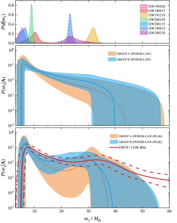
Figure 1: Top panel: one-dimensional posterior distributions for the masses of the BHs in O3 GW NSBH candidates. Middle and bottom panels: the BH mass distributions inferred for the power-law and power-law+peak models. Orange (blue) solid line and shaded region represent the median and $90\%$ confidence interval obtained by adopting group a (group b), respectively. Red lines are the GWTC-3 BBH primary mass distribution (The LIGO Scientific Collaboration et al., 2021a) with the median (solid) and $90\%$ confidence interval (dashed).

Figure 1 displays the posterior distribution of the primary BH masses for O3 NSBH candidates. Taken uniform model as a fixed model for the NS mass distribution, the BH mass distribution inferred by the power-law and power-law+peak models for both groups of NSBH events are also plotted in Figure 1 as examples.

When we fit the power-law BH mass distribution model to the data of group a, the power-law index is $\alpha=2.7^{+2.0}_{-1.5}$ between the sharp low-mass cutoff $m_{\rm 1,min}=5.3^{+1.1}_{-1.7}\,M_{\odot}$ and high-mass cutoff $m_{\rm 1,max}=44^{+14}_{-12}\,M_{\odot}$. Since the primary masses of GW190814 and GW200210 are larger than those of other NSBHs expect GW191219, if we include them in the data, the mass model would have a relatively shallower slope with $\alpha=1.7^{+1.3}_{-1.3}$ from $m_{\rm 1,min}=5.1^{+1.1}_{-1.7}\,M_{\odot}$ to $m_{\rm 1,max}=40^{+17}_{-8}\,M_{\odot}$. $m_{\rm 1,max}$ depends on the priors, but the lower bound on $m_{\rm 1,max}$ is driven by the precise mass measurement for $\sim 32\,M_{\odot}$ primary of GW191219.

The power-law model may be disfavored to explain the mass distribution of BHs in NSBH systems due to the lack of NSBH GW detections with a primary BH mass in the range of $\sim 12-20\,M_{\odot}$, so that a more complicated BH mass distribution model with the consideration of bimodal components is needed. For different NS mass distribution models and groups of NSBH events, the results of log Bayes factor (see Table 3) reveal that the power-law+peak model of the BH mass distribution has a moderate preference over the power-law model by a Bayes factor of $\sim 2:1-4:1$ ($\log_{10}\mathcal{B}\sim 0.4-0.6$). For group a (group b), we find a power-law slope of $\alpha=4.8^{+4.5}_{-2.8}$ ($\alpha=4.0^{+5.1}_{-2.7}$), supplemented by a Gaussian peak at $\mu_{m}=33^{+14}_{-9}\,M_{\odot}$ ($\mu_{m}=27^{+15}_{-6}\,M_{\odot}$), between minimum mass $m_{\rm 1,min}=5.7^{+1.1}_{-1.3}\,M_{\odot}$ ($m_{\rm 1,min}=5.6^{+1.1}_{-1.5}\,M_{\odot}$) and maximum mass $m_{\rm 1,max}=38^{+19}_{-7}\,M_{\odot}$ ($m_{\rm 1,max}=39^{+18}_{-9}\,M_{\odot}$). Comparing with those inferred from the power-law model, the BH mass distribution derived by the power-law+peak model would have steeper slopes, but obtain consistent minimum and maximum masses.

The LIGO Scientific Collaboration et al. (2021a) showed that the power-law+peak model can also well fit to the primary mass of GWTC-3 BBH GW events. They found that the primary mass distribution of BBH, plotted in the bottom panel of Figure 1, would have a power-law slope of $\alpha=3.4^{+0.58}_{-0.49}$ with a Gaussian peak at $\mu_{m}=34^{+2.3}_{-3.8}\,M_{\odot}$. The comparison of the primary mass distributions by the GW detections indicate that the primary components of cosmological NSBH and BBH mergers could have similar minimum mass distributions and similar power-law slopes. The maximum primary mass of NSBH mergers is much lower than that of BBH mergers because of the present limited number of detections for high-mass NSBH mergers. Constrained by group a, the primary BH of GW191219 dominates the high-mass component, which would result in a similar mean of the Gaussian component and a similar probability distribution compared with those of BBH mergers. The similar shapes of the primary BH mass distribution between GW NSBH and BBH mergers indicate that the NSBH mergers reported in GWTC-3 are likely credible and plausibly have an astrophysical origin. When we include GW190814 and GW200210, the mean of the Gaussian component is less massive than that of GWTC-3 BBH mergers.

3.2 NS Mass Distribution

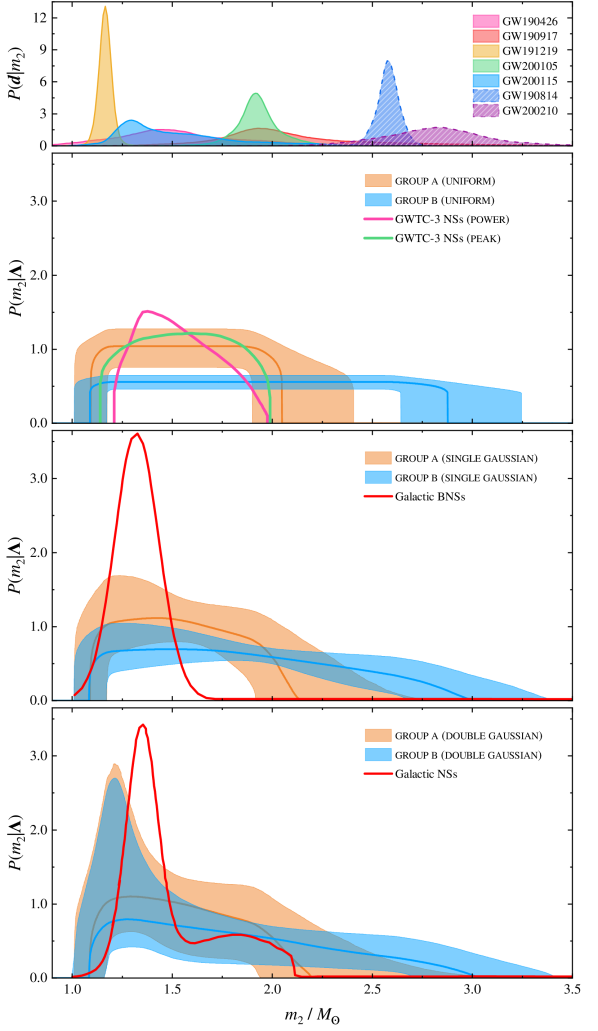
Figure 2: Top panel: one-dimensional posterior distributions for the masses of the NSs in O3 GW NSBH candidates. Following three panels: the NS mass distributions inferred for the uniform, single gaussian and double gaussian models. The orange (blue) solid lines and shaded regions represent the median with the $90\%$ confidence interval by adopting the data of group a (group b), respectively. Derived by The LIGO Scientific Collaboration et al. (2021a), the pink and green lines are the median mass distribution of the NSs in GW BNS and NSBH mergers using power and peak models. The red lines shown in the single gaussian and double gaussian models are the NS masses of galactic BNSs (Kiziltan et al., 2013) and galactic NSs (Farr & Chatziioannou, 2020).

The top panel of Figure 2 shows the posterior distribution of the secondary NS masses for O3 NSBH candidates. Furthermore, by setting power-law+peak model as a fiducial model for BH mass distribution, we plot the medians and 90% confidence intervals of the inferred NS mass distributions for the uniform, single gaussian, and double gaussian models in Figure 2.

Given the data of group a, three models exhibit a similar fitting result for the NS mass distribution. All models show a consistent minimum NS mass, $m_{\rm 2,min}=1.088^{+0.086}_{-0.076}\,M_{\odot}$. The maximum NS mass inferred by the uniform model is $m_{\rm 2,max}=2.04^{+0.35}_{-0.15}\,M_{\odot}$, while $m_{\rm 2,max}$ would be a little higher and broader, i.e., $m_{\rm 2,max}=2.1^{+1.0}_{-0.2}\,M_{\odot}$ and $m_{\rm 2,max}=2.2^{+1.1}_{-0.3}\,M_{\odot}$, if one respectively considers the single gaussian and double gaussian NS mass models. Regardless of which prior models one adopts, the final NS mass distributions look like a uniform distribution between minimum and maximum masses.

Using group b as the observational input, by a Bayes factor of $\sim 2:1-3:1$ $(\log_{10}\mathcal{B}\sim 0.3-0.5)$, the double gaussian model provides a better fit than the uniform and single gaussian models to the shape of the NS mass distribution. The fitting results of double gaussian model are $\mu_{1}=1.30^{+0.57}_{-0.21}\,M_{\odot}$, $\sigma_{1}=0.61^{+0.76}_{-0.52}\,M_{\odot}$, $\mu_{2}=2.04^{+0.85}_{-0.72}\,M_{\odot}$, and $\sigma_{2}=0.94^{+0.50}_{-0.71}\,M_{\odot}$. However, the inferred NS mass distribution does not show apparent bimodal structures but presents a linear decline to the maximum mass after the peak. Due to the presence of two other events (i.e., GW190814 and GW200210) with a high-mass secondary, the maximum mass would be much higher with a larger uncertainty compared with the result inferred by the input of group a, i.e., $m_{\rm 2,max}=3.02^{+0.40}_{-0.33}\,M_{\odot}$.

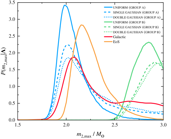
Figure 3: Maximum mass distribution for the NSs in GW NSBH binaries. Blue (green) solid, dashed and dotted lines show the inferred maximum mass distribution by adopting uniform, single gaussian, and double gaussian models for the data of group a (group b), respectively. The red and orange lines represent the maximum mass derived from the Galactic NS population in Farr & Chatziioannou (2020) and the maximum TOV mass from the EoS predicted by Landry et al. (2020).

In view of the lack of observations for Galactic NSBH binaries, we briefly compare our results of NS masses with the mass distributions of the galactic BNSs (Kiziltan et al., 2013), Galactic NSs (Farr & Chatziioannou, 2020), and GW NSs reported in GWTC-3 (The LIGO Scientific Collaboration et al., 2021a). As shown in Figure 2, in comparison with the Galactic BNSs and NSs that have a narrow mass distribution in the low-mass region, the mass distribution of NSs observed in GW NSBH mergers is broader and has greater prevalence for high-mass NSs. This may be because NSBH systems with high-mass NSs could merge early, and hence, predominantly low-mass NSs remain observed in our Galaxy. Furthermore, GW NSs reported by The LIGO Scientific Collaboration et al. (2021a) and our fitting NSs in GW NSBH binaries similarly show a broad, relatively flat mass distribution.

The Galactic NS population (Farr & Chatziioannou, 2020) and the maximum Tolman-Oppenheimer-Volkov (TOV) mass predicted by Landry et al. (2020) gave the value of $m_{\rm 2,max}=2.3^{+0.8}_{-0.3}\,M_{\odot}$ and $m_{\rm TOV}=2.2^{+0.4}_{-0.2}\,M_{\odot}$, respectively. These constrained masses have a good consistency with our maximum masses of NSs inferred by the data of group a. As illustrated in Figure 3, if we also take GW190814 and GW200219 into consideration, the simulated maximum mass would be always larger than $\sim 2.5\,M_{\odot}$ and peak at $\sim 2.7-3.0\,M_{\odot}$. The overlap between the maximum NS mass in GW NSBH binaries and the maximum masses observed in the Galaxy would be limited. The secondary maximum mass in the GW NSBH mergers would significantly deviate from that inferred from the NSs in our Galaxy.

3.3 Spin Distribution

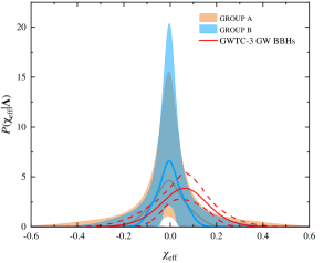
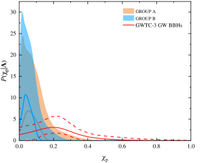
Figure 4: Population distributions for $\chi_{\rm eff}$ (left panel) and $\chi_{\rm p}$ (right panel) of NSBH systems. Orange and blue shaded regions show the central $90\%$ credible bounds using group a and group b, while the solid lines show the median posterior prediction. The red solid and dashed lines mark the central $50\%$ and $90\%$ posterior credible regions for O3 GW BBH systems from The LIGO Scientific Collaboration et al. (2021a), respectively

Figure 4 illustrates our example constraints on the $\chi_{\rm eff}$ and $\chi_{\rm p}$ distributions under the models of the power-law+peak BH mass distribution, the uniform NS mass distribution, and the gaussian spin distribution. Regardless of the prior models that we choose, our constrained results reveal that both $\chi_{\rm eff}$ and $\chi_{\rm p}$ of NSBH mergers could have near-zero distributions. However, due to the limited number of detections in O3, the spin distributions display large uncertainties.

For the data of group a, the posterior distributions of the median and the standard deviation of $\chi_{\rm eff}$ ($\chi_{\rm p}$) are $\mu_{\rm eff}=-0.004^{+0.046}_{-0.053}$ ($\mu_{\rm p}=0.064^{+0.084}_{-0.049}$) and $\sigma_{\rm eff}=0.07^{+0.18}_{-0.06}$ ($\sigma_{\rm p}=0.03^{+0.10}_{-0.02}$), respectively. group b data further support a negligible spin distribution. In this case, we obtain $\mu_{\rm eff}=-0.003^{+0.030}_{-0.035}$ ($\mu_{\rm p}=0.046^{+0.056}_{-0.033}$) and $\sigma_{\rm eff}=0.05^{+0.11}_{-0.04}$ ($\sigma_{\rm p}=0.024^{+0.061}_{-0.013}$). All of these individual GW candidates, except for GW200115, have near-zero $\chi_{\rm eff}$ and $\chi_{\rm p}$. It is expected that removing some of the marginal events would not significantly affect the spin population distributions. Because the spin of the BH component contributes to most of $\chi_{\rm eff}$ and $\chi_{\rm p}$, the measurements of negligible spin distribution indicate that BHs in cosmological NSBH systems could have a low-spin population distribution.

In Figure 4, we also show the comparison with the resulting spin distributions of BBH mergers made with GWTC-3 (The LIGO Scientific Collaboration et al., 2021a) using the gaussian spin model. The spin measurements for BBH mergers suggested an effective inspiral spin distribution of non-vanishing width centered at $\chi_{\rm eff}=0.06^{+0.04}_{-0.04}$ and a narrow precession spin distribution centered around $\chi_{\rm p}\approx 0.2$. By contrast, the population distributions of $\chi_{\rm eff}$ and $\chi_{\rm p}$ for NSBH systems are lower than those of BBH systems.

3.4 Event Rate

GWTC-3 reported a NSBH merger rate of $7.4-320.0\,{\rm Gpc}^{-3}\,{\rm yr}^{-1}$. In our work, the inferred merger rate mainly depends on the adopted input of observational data. By setting powerlaw+peak as the BH mass model and uniform as the NS mass model, for group a, different mass models give a consistent NSBH rate merger, which is $13.2-64.9\,{\rm Gpc}^{-3}\,{\rm yr}^{-1}$. If GW190814 and GW200210 were NSBH mergers, the uncertainty of the NSBH rate merger would be lower, i.e., $13.8-53.0\,{\rm yr}^{-1}$. The inferred event rate does not increase since the low-mass end of the BH mass spectrum is relatively unaffected by these two additional events for the powerlaw+peak model as they would be picked up by the high-mass peak component.

4 Discussion

4.1 Tidal Disruption Probability

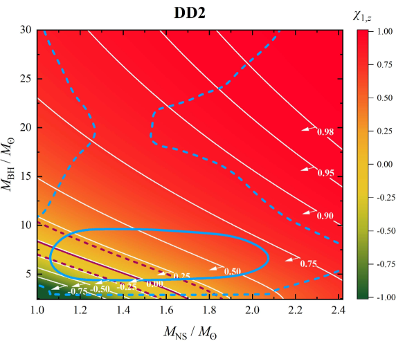
Figure 5: The source-frame mass parameter space where tidal disruption can occur by considering the specific NS EoS DD2. We mark several values of primary BH spin along the orbital angular momentum from $\chi_{1,z}=-0.75$ to $\chi_{1,z}=0.98$ as solid white lines. For a specific $\chi_{1,z}$, the NSBH mergers with component masses located at the bottom left parameter space (denoted by the direction of the arrows) can allow tidal disruptions to occur. The blue solid and dashed lines represent $50\%$ and $90\%$ source-frame masses distributions of inferred population results for O3 GW NSBH mergers. The dark purple solid and dashed lines represent median and $90\%$ distributions of $\chi_{1,z}$, respectively.

We calculate the amount of total baryon mass after NSBH mergers, which is mainly determined by BH mass, BH aligned spin, NS mass, and NS EoS, to judge whether or not tidal disruption happens using an empirical model presented by Foucart et al. (2018). We generate cosmological NSBH merger events based on the posterior results obtained by the power-law+peak BH mass distribution and the single gaussian NS mass distribution for the observational input of group a. For each posterior population sample, we simulate 1000 events including the system parameters of BH mass, NS mass, and effective spin. It is plausibly expected that most NSs would have near-zero spins before NSBH mergers owing to the spindown process via magnetic dipole radiation (e.g., Manchester et al., 2005; Osłowski et al., 2011). The primary BH spin along the orbital angular momentum can be thus estimated as $\chi_{1,z}\approx(m_{1}+m_{2})\chi_{\rm eff}/m_{1}$. A NS EoS of DD2 (Typel et al., 2010) is adopted, since this EoS is one of the stiffest EoSs constrained by GW170817 (Abbott et al., 2018, 2019b; Dietrich et al., 2020).

Figure 5 shows the parameter space where the NS can be tidally disrupted. The 50% and 90% distributions of BH mass, NS mass, and BH aligned spin for our simulated NSBH mergers are also plotted in Figure 5. Because the simulated BHs have a common aligned spin in the range of $-0.25\lesssim\chi_{1,z}\lesssim 0.25$, the mass space that allows NS tidal disruption and produce bright EM signals would require $m_{1}\lesssim 7\,M_{\odot}$ and $m_{2}\lesssim 1.5\,M_{\odot}$. However, most of our simulated NSBH mergers inferred from the GW observations have BHs and NSs located outside of the tidal disruption mass space. This indicates that plunging events would account for a large fractional of cosmological NSBH mergers.

4.2 Implications for the Formation Channel

Among O3 NSBH candidates, Abbott et al. (2021a) reported that the BH component of GW200115 could have a misaligned spin and an orbital precession. Recently, many works in the literature, e.g., Broekgaarden & Berger (2021); Fragione et al. (2021); Gompertz et al. (2021); Zhu (2021), presented that a moderate or strong natal kick for the BH or the NS is required in order to produce the observed misalignment angle of GW200115. On the other hand, applying alternative astrophysically motivated priors to GW200115, Mandel & Smith (2021) constrained the BH spin to be centered at zero. It would thus result in a more negligible population spin distribution.

The most promising formation scenario for NSBH binaries is isolated binary evolution (e.g., Broekgaarden et al., 2021; Shao & Li, 2021). Furthermore, a small fraction of NSBH binaries are believed to result from dynamical evolution (e.g., Clausen et al., 2013; Ye et al., 2020). In the standard scenario for merging NSBH formation through isolated binary evolution, the primary (initially more massive star) evolves off the main sequence, initiates mass transfer onto the secondary, and finally collapses to form a BH before the common-envelope phase. During this process, the primary evolves in a wide orbit in which the tides are too weak to spin it up. Additionally, the angular momentum content of the primary is reduced by stripping off its outer layers due to stellar winds and mass transfer via the first Lagrangian point onto its companion. Furthermore, under the assumption of efficient angular momentum transport within the star, predicted by the Tayler-Spruit dynamo (Spruit, 2002) or its revised version by Fuller et al. (2019), the spin of the first-born BH is found to be small (Qin et al., 2018; Belczynski et al., 2020; Drozda et al., 2020). Our present results for constraints on the spin population properties of GW NSBH mergers would strongly support the standard scenario for the formation of cosmological NSBH binaries.

Alternatively, the first-born compact object in NSBH mergers could be a NS. Román-Garza et al. (2021) recently claimed that the fraction of the systems with a first-born NS with different supernova engines is $\sim 10\%$. This scenario would lead to a group of NSBH mergers with a unique spin distribution (Hu et al., 2022), which has not been discovered by present GW detections. Zhu et al. (2021e) further found that the brightness of kilonova is strongly dependent on the spin magnitude of the BH in the NSBH mergers. The possible energy injection from BH-torus would also be affected by the primary BH spin (e.g., Ma et al., 2018; Qi et al., 2021). Therefore, we suggest a detailed investigation of the BH spin-dependent parameter space in the near future.

5 Conclusions

In this work, we analyse the canonical results of these confirmed NSBH candidates reported by LVK Collaboration by employing a Bayesian framework to study the population properties of GW NHBH mergers. A power-law with an Gaussian peak model can well explain the NSBH primary mass distribution. The posterior distribution of the power-law index ($\alpha=4.8^{+4.5}_{-2.8}$), the minimum mass ($m_{\rm 1,min}=5.3^{+1.1}_{-1.7}$), and the mean of the Gaussian feature ($\mu_{m}=33^{+14}_{-9}\,M_{\odot}$) have similar properties with those of GWTC-3 BBH primary mass distribution. The mass distribution of the NS component is consistent with a uniform distribution between $\sim 1.0-2.1\,M_{\odot}$, similar to the constraint on the masses of NSs in GW binaries (Landry & Read, 2021; The LIGO Scientific Collaboration et al., 2021a). The maximum mass distribution derived by GW NSBH mergers agrees with that inferred from the NSs in our Galaxy. If these NSBH candidates reported by LVK Collaboration are of an astrophysical origin, the event rate of NSBH mergers would be $13.2-64.9\,{\rm Gpc}^{-3}\,{\rm yr}^{-1}$.

If GW190814 and GW200210 are NSBH mergers, the BH mass spectrum can be also fitted by a power-law distribution with a high-mass Gaussian component. A double gaussian model is supported to account for the NS mass distribution. However, the inferred NS mass distribution does not show apparent bimodal structures, which performs a linear decline to the maximum mass after the peak of $\sim 1.3\,M_{\odot}$. The secondary maximum mass in the GW NSBH mergers would significantly increase and result in an apparent deviation from that inferred from the NSs in our Galaxy. The event rate of NSBH mergers would change to $13.8-53.0\,{\rm Gpc}^{-3}\,{\rm yr}^{-1}$.

Different from GWTC-3 BBH systems that show non-vanishing distributions of spins, GW NSBH systems display near-zero distributions for both effective inspiral spin and effective precession spin. Because the NS component makes an insignificant contribution to the spin of the system, the negligible spin distributions for NSBH populations plausibly indicate that most BHs in the cosmological NSBH systems would have a low spin. This result would support the standard isolated formation channel of NSBH binaries. Since the primary BHs likely have low spins, plunging events would be the dominant population for NSBH mergers and hence no bright EM counterparts are expected for most of NSBH mergers.

We have assumed that GWTC-3 NSBH candidates are real signals of astrophysical origins when we analyse the population properties of GW NSBH mergers. Interestingly, (1) the similar shapes of the primary BH mass distribution between GW NSBH and BBH mergers, (2) the consistent shapes of the NS mass distribution between NS mergers and NSBH mergers, (3) near-zero spin distributions for NSBH populations which are supported by the standard isolated formation channel of NSBH binaries, indicate that the NSBH mergers reported in GWTC-3 are likely credible and plausibly real signals with astrophysical origins. In the fourth observation run, more discovered NSBH mergers would help to more precisely model the population properties of cosmological NSBH mergers.

References

- Abbott et al. (2017a) Abbott, B. P., Abbott, R., Abbott, T. D., et al. 2017a, Phys. Rev. Lett., 119, 161101, doi: 10.1103/PhysRevLett.119.161101
- Abbott et al. (2017b) —. 2017b, ApJ, 848, L13, doi: 10.3847/2041-8213/aa920c
- Abbott et al. (2017c) —. 2017c, ApJ, 848, L12, doi: 10.3847/2041-8213/aa91c9
- Abbott et al. (2018) —. 2018, Phys. Rev. Lett., 121, 161101, doi: 10.1103/PhysRevLett.121.161101
- Abbott et al. (2019a) —. 2019a, ApJ, 882, L24, doi: 10.3847/2041-8213/ab3800
- Abbott et al. (2019b) —. 2019b, Physical Review X, 9, 011001, doi: 10.1103/PhysRevX.9.011001
- Abbott et al. (2020) Abbott, R., Abbott, T. D., Abraham, S., et al. 2020, ApJ, 896, L44, doi: 10.3847/2041-8213/ab960f
- Abbott et al. (2021a) —. 2021a, ApJ, 915, L5, doi: 10.3847/2041-8213/ac082e
- Abbott et al. (2021b) —. 2021b, Physical Review X, 11, 021053, doi: 10.1103/PhysRevX.11.021053
- Abbott et al. (2021c) —. 2021c, ApJ, 913, L7, doi: 10.3847/2041-8213/abe949
- Acernese et al. (2015) Acernese, F., Agathos, M., Agatsuma, K., et al. 2015, Classical and Quantum Gravity, 32, 024001, doi: 10.1088/0264-9381/32/2/024001
- Alexander et al. (2021) Alexander, K. D., Schroeder, G., Paterson, K., et al. 2021, arXiv e-prints, arXiv:2102.08957. https://arxiv.org/abs/2102.08957
- Alsing et al. (2018) Alsing, J., Silva, H. O., & Berti, E. 2018, MNRAS, 478, 1377, doi: 10.1093/mnras/sty1065
- Anand et al. (2021) Anand, S., Coughlin, M. W., Kasliwal, M. M., et al. 2021, Nature Astronomy, 5, 46, doi: 10.1038/s41550-020-1183-3
- Antoniadis et al. (2016) Antoniadis, J., Tauris, T. M., Ozel, F., et al. 2016, arXiv e-prints, arXiv:1605.01665. https://arxiv.org/abs/1605.01665
- Arcavi et al. (2017) Arcavi, I., Hosseinzadeh, G., Howell, D. A., et al. 2017, Nature, 551, 64, doi: 10.1038/nature24291
- Aso et al. (2013) Aso, Y., Michimura, Y., Somiya, K., et al. 2013, Phys. Rev. D, 88, 043007, doi: 10.1103/PhysRevD.88.043007
- Barbieri et al. (2019) Barbieri, C., Salafia, O. S., Perego, A., Colpi, M., & Ghirlanda, G. 2019, A&A, 625, A152, doi: 10.1051/0004-6361/201935443
- Belczynski et al. (2008) Belczynski, K., Taam, R. E., Rantsiou, E., & van der Sluys, M. 2008, ApJ, 682, 474, doi: 10.1086/589609
- Belczynski et al. (2020) Belczynski, K., Klencki, J., Fields, C. E., et al. 2020, A&A, 636, A104, doi: 10.1051/0004-6361/201936528
- Broekgaarden & Berger (2021) Broekgaarden, F. S., & Berger, E. 2021, ApJ, 920, L13, doi: 10.3847/2041-8213/ac2832
- Broekgaarden et al. (2021) Broekgaarden, F. S., Berger, E., Neijssel, C. J., et al. 2021, MNRAS, 508, 5028, doi: 10.1093/mnras/stab2716
- Cheng & Wang (1999) Cheng, K. S., & Wang, J.-M. 1999, ApJ, 521, 502, doi: 10.1086/307572
- Clausen et al. (2013) Clausen, D., Sigurdsson, S., & Chernoff, D. F. 2013, MNRAS, 428, 3618, doi: 10.1093/mnras/sts295
- Coughlin et al. (2020) Coughlin, M. W., Dietrich, T., Antier, S., et al. 2020, MNRAS, 497, 1181, doi: 10.1093/mnras/staa1925
- Coulter et al. (2017) Coulter, D. A., Foley, R. J., Kilpatrick, C. D., et al. 2017, Science, 358, 1556, doi: 10.1126/science.aap9811
- Dai (2019) Dai, Z. G. 2019, ApJ, 873, L13, doi: 10.3847/2041-8213/ab0b45
- Dietrich et al. (2020) Dietrich, T., Coughlin, M. W., Pang, P. T. H., et al. 2020, Science, 370, 1450, doi: 10.1126/science.abb4317
- Dobie et al. (2021) Dobie, D., Stewart, A., Hotokezaka, K., et al. 2021, arXiv e-prints, arXiv:2109.08452. https://arxiv.org/abs/2109.08452
- D’Orazio et al. (2021) D’Orazio, D. J., Haiman, Z., Levin, J., Samsing, J., & Vigna-Gomez, A. 2021, arXiv e-prints, arXiv:2112.01979. https://arxiv.org/abs/2112.01979
- Drout et al. (2017) Drout, M. R., Piro, A. L., Shappee, B. J., et al. 2017, Science, 358, 1570, doi: 10.1126/science.aaq0049
- Drozda et al. (2020) Drozda, P., Belczynski, K., O’Shaughnessy, R., Bulik, T., & Fryer, C. L. 2020, arXiv e-prints, arXiv:2009.06655. https://arxiv.org/abs/2009.06655
- Eichler et al. (1989) Eichler, D., Livio, M., Piran, T., & Schramm, D. N. 1989, Nature, 340, 126, doi: 10.1038/340126a0
- Evans et al. (2017) Evans, P. A., Cenko, S. B., Kennea, J. A., et al. 2017, Science, 358, 1565, doi: 10.1126/science.aap9580
- Farah et al. (2021) Farah, A. M., Fishbach, M., Essick, R., Holz, D. E., & Galaudage, S. 2021, arXiv e-prints, arXiv:2111.03498. https://arxiv.org/abs/2111.03498
- Farr & Chatziioannou (2020) Farr, W. M., & Chatziioannou, K. 2020, Research Notes of the American Astronomical Society, 4, 65, doi: 10.3847/2515-5172/ab9088
- Farr et al. (2015) Farr, W. M., Gair, J. R., Mandel, I., & Cutler, C. 2015, Phys. Rev. D, 91, 023005, doi: 10.1103/PhysRevD.91.023005
- Fernández et al. (2015) Fernández, R., Kasen, D., Metzger, B. D., & Quataert, E. 2015, MNRAS, 446, 750, doi: 10.1093/mnras/stu2112
- Fishbach & Holz (2017) Fishbach, M., & Holz, D. E. 2017, ApJ, 851, L25, doi: 10.3847/2041-8213/aa9bf6
- Fishbach et al. (2018) Fishbach, M., Holz, D. E., & Farr, W. M. 2018, ApJ, 863, L41, doi: 10.3847/2041-8213/aad800
- Foucart (2012) Foucart, F. 2012, Phys. Rev. D, 86, 124007, doi: 10.1103/PhysRevD.86.124007
- Foucart et al. (2018) Foucart, F., Hinderer, T., & Nissanke, S. 2018, Phys. Rev. D, 98, 081501, doi: 10.1103/PhysRevD.98.081501
- Fragione (2021) Fragione, G. 2021, arXiv e-prints, arXiv:2110.09604. https://arxiv.org/abs/2110.09604
- Fragione & Loeb (2021) Fragione, G., & Loeb, A. 2021, MNRAS, 503, 2861, doi: 10.1093/mnras/stab666
- Fragione et al. (2021) Fragione, G., Loeb, A., & Rasio, F. A. 2021, ApJ, 918, L38, doi: 10.3847/2041-8213/ac225a
- Fuller et al. (2019) Fuller, J., Piro, A. L., & Jermyn, A. S. 2019, MNRAS, 485, 3661, doi: 10.1093/mnras/stz514
- Ghirlanda et al. (2019) Ghirlanda, G., Salafia, O. S., Paragi, Z., et al. 2019, Science, 363, 968, doi: 10.1126/science.aau8815
- Goldstein et al. (2017) Goldstein, A., Veres, P., Burns, E., et al. 2017, ApJ, 848, L14, doi: 10.3847/2041-8213/aa8f41
- Gompertz et al. (2021) Gompertz, B. P., Nicholl, M., Schmidt, P., Pratten, G., & Vecchio, A. 2021, arXiv e-prints, arXiv:2108.10184. https://arxiv.org/abs/2108.10184
- Gompertz et al. (2020) Gompertz, B. P., Cutter, R., Steeghs, D., et al. 2020, MNRAS, 497, 726, doi: 10.1093/mnras/staa1845
- Hannam et al. (2014) Hannam, M., Schmidt, P., Bohé, A., et al. 2014, Phys. Rev. Lett., 113, 151101, doi: 10.1103/PhysRevLett.113.151101
- Hu et al. (2022) Hu, R.-C., Zhu, J.-P., Qin, Y., et al. 2022, arXiv e-prints, arXiv:2201.09549. https://arxiv.org/abs/2201.09549
- Kasliwal et al. (2017) Kasliwal, M. M., Nakar, E., Singer, L. P., et al. 2017, Science, 358, 1559, doi: 10.1126/science.aap9455
- Kasliwal et al. (2020) Kasliwal, M. M., Anand, S., Ahumada, T., et al. 2020, ApJ, 905, 145, doi: 10.3847/1538-4357/abc335
- Kawaguchi et al. (2015) Kawaguchi, K., Kyutoku, K., Nakano, H., et al. 2015, Phys. Rev. D, 92, 024014, doi: 10.1103/PhysRevD.92.024014
- Kawaguchi et al. (2016) Kawaguchi, K., Kyutoku, K., Shibata, M., & Tanaka, M. 2016, ApJ, 825, 52, doi: 10.3847/0004-637X/825/1/52
- Kilpatrick et al. (2017) Kilpatrick, C. D., Foley, R. J., Kasen, D., et al. 2017, Science, 358, 1583, doi: 10.1126/science.aaq0073
- Kilpatrick et al. (2021) Kilpatrick, C. D., Coulter, D. A., Arcavi, I., et al. 2021, arXiv e-prints, arXiv:2106.06897. https://arxiv.org/abs/2106.06897
- Kiziltan et al. (2013) Kiziltan, B., Kottas, A., De Yoreo, M., & Thorsett, S. E. 2013, ApJ, 778, 66, doi: 10.1088/0004-637X/778/1/66
- Krüger & Foucart (2020) Krüger, C. J., & Foucart, F. 2020, Phys. Rev. D, 101, 103002, doi: 10.1103/PhysRevD.101.103002
- Kyutoku et al. (2015) Kyutoku, K., Ioka, K., Okawa, H., Shibata, M., & Taniguchi, K. 2015, Phys. Rev. D, 92, 044028, doi: 10.1103/PhysRevD.92.044028
- Kyutoku et al. (2013) Kyutoku, K., Ioka, K., & Shibata, M. 2013, Phys. Rev. D, 88, 041503, doi: 10.1103/PhysRevD.88.041503
- Kyutoku et al. (2011) Kyutoku, K., Okawa, H., Shibata, M., & Taniguchi, K. 2011, Phys. Rev. D, 84, 064018, doi: 10.1103/PhysRevD.84.064018
- Landry et al. (2020) Landry, P., Essick, R., & Chatziioannou, K. 2020, Phys. Rev. D, 101, 123007, doi: 10.1103/PhysRevD.101.123007
- Landry & Read (2021) Landry, P., & Read, J. S. 2021, ApJ, 921, L25, doi: 10.3847/2041-8213/ac2f3e
- Lattimer (2012) Lattimer, J. M. 2012, Annual Review of Nuclear and Particle Science, 62, 485, doi: 10.1146/annurev-nucl-102711-095018
- Lazzati et al. (2018) Lazzati, D., Perna, R., Morsony, B. J., et al. 2018, Phys. Rev. Lett., 120, 241103, doi: 10.1103/PhysRevLett.120.241103
- Li & Paczyński (1998) Li, L.-X., & Paczyński, B. 1998, ApJ, 507, L59, doi: 10.1086/311680
- Li & Shen (2021) Li, Y., & Shen, R.-F. 2021, ApJ, 911, 87, doi: 10.3847/1538-4357/abe462
- Li et al. (2021) Li, Y.-J., Tang, S.-P., Wang, Y.-Z., et al. 2021, arXiv e-prints, arXiv:2108.06986. https://arxiv.org/abs/2108.06986
- LIGO Scientific Collaboration (2018) LIGO Scientific Collaboration. 2018, LIGO Algorithm Library - LALSuite, free software (GPL), doi: 10.7935/GT1W-FZ16
- LIGO Scientific Collaboration et al. (2015) LIGO Scientific Collaboration, Aasi, J., Abbott, B. P., et al. 2015, Classical and Quantum Gravity, 32, 074001, doi: 10.1088/0264-9381/32/7/074001
- Lyman et al. (2018) Lyman, J. D., Lamb, G. P., Levan, A. J., et al. 2018, Nature Astronomy, 2, 751, doi: 10.1038/s41550-018-0511-3
- Ma et al. (2018) Ma, S.-B., Lei, W.-H., Gao, H., et al. 2018, ApJ, 852, L5, doi: 10.3847/2041-8213/aaa0cd
- Manchester et al. (2005) Manchester, R. N., Hobbs, G. B., Teoh, A., & Hobbs, M. 2005, AJ, 129, 1993, doi: 10.1086/428488
- Mandel et al. (2019) Mandel, I., Farr, W. M., & Gair, J. R. 2019, MNRAS, 486, 1086, doi: 10.1093/mnras/stz896
- Mandel & Smith (2021) Mandel, I., & Smith, R. J. E. 2021, arXiv e-prints, arXiv:2109.14759. https://arxiv.org/abs/2109.14759
- Margutti et al. (2017) Margutti, R., Berger, E., Fong, W., et al. 2017, ApJ, 848, L20, doi: 10.3847/2041-8213/aa9057
- McKernan et al. (2020) McKernan, B., Ford, K. E. S., & O’Shaughnessy, R. 2020, MNRAS, 498, 4088, doi: 10.1093/mnras/staa2681
- Metzger et al. (2010) Metzger, B. D., Martínez-Pinedo, G., Darbha, S., et al. 2010, MNRAS, 406, 2650, doi: 10.1111/j.1365-2966.2010.16864.x
- Miller et al. (2020) Miller, S., Callister, T. A., & Farr, W. M. 2020, ApJ, 895, 128, doi: 10.3847/1538-4357/ab80c0
- Narayan et al. (1992) Narayan, R., Paczynski, B., & Piran, T. 1992, ApJ, 395, L83, doi: 10.1086/186493
- Nitz et al. (2021) Nitz, A. H., Kumar, S., Wang, Y.-F., et al. 2021, arXiv e-prints, arXiv:2112.06878. https://arxiv.org/abs/2112.06878
- Osłowski et al. (2011) Osłowski, S., Bulik, T., Gondek-Rosińska, D., & Belczyński, K. 2011, MNRAS, 413, 461, doi: 10.1111/j.1365-2966.2010.18147.x
- Özel et al. (2010) Özel, F., Psaltis, D., Narayan, R., & McClintock, J. E. 2010, ApJ, 725, 1918, doi: 10.1088/0004-637X/725/2/1918
- Paczynski (1986) Paczynski, B. 1986, ApJ, 308, L43, doi: 10.1086/184740
- Paczynski (1991) —. 1991, Acta Astron., 41, 257
- Page et al. (2020) Page, K. L., Evans, P. A., Tohuvavohu, A., et al. 2020, MNRAS, 499, 3459, doi: 10.1093/mnras/staa3032
- Pan & Yang (2019) Pan, Z., & Yang, H. 2019, Phys. Rev. D, 100, 043025, doi: 10.1103/PhysRevD.100.043025
- Perna et al. (2021) Perna, R., Lazzati, D., & Cantiello, M. 2021, ApJ, 906, L7, doi: 10.3847/2041-8213/abd319
- Pian et al. (2017) Pian, E., D’Avanzo, P., Benetti, S., et al. 2017, Nature, 551, 67, doi: 10.1038/nature24298
- Pratten et al. (2021) Pratten, G., García-Quirós, C., Colleoni, M., et al. 2021, Phys. Rev. D, 103, 104056, doi: 10.1103/PhysRevD.103.104056
- Qi et al. (2021) Qi, Y.-Q., Liu, T., Huang, B.-Q., Wei, Y.-F., & Bu, D.-F. 2021, arXiv e-prints, arXiv:2111.03812. https://arxiv.org/abs/2111.03812
- Qin et al. (2018) Qin, Y., Fragos, T., Meynet, G., et al. 2018, A&A, 616, A28, doi: 10.1051/0004-6361/201832839
- Raaijmakers et al. (2021) Raaijmakers, G., Nissanke, S., Foucart, F., et al. 2021, ApJ, 922, 269, doi: 10.3847/1538-4357/ac222d
- Román-Garza et al. (2021) Román-Garza, J., Bavera, S. S., Fragos, T., et al. 2021, ApJ, 912, L23, doi: 10.3847/2041-8213/abf42c
- Roulet et al. (2020) Roulet, J., Venumadhav, T., Zackay, B., Dai, L., & Zaldarriaga, M. 2020, Phys. Rev. D, 102, 123022, doi: 10.1103/PhysRevD.102.123022
- Savchenko et al. (2017) Savchenko, V., Ferrigno, C., Kuulkers, E., et al. 2017, ApJ, 848, L15, doi: 10.3847/2041-8213/aa8f94
- Shao et al. (2020) Shao, D.-S., Tang, S.-P., Jiang, J.-L., & Fan, Y.-Z. 2020, Phys. Rev. D, 102, 063006, doi: 10.1103/PhysRevD.102.063006
- Shao & Li (2021) Shao, Y., & Li, X.-D. 2021, ApJ, 920, 81, doi: 10.3847/1538-4357/ac173e
- Smartt et al. (2017) Smartt, S. J., Chen, T. W., Jerkstrand, A., et al. 2017, Nature, 551, 75, doi: 10.1038/nature24303
- Speagle (2020) Speagle, J. S. 2020, MNRAS, 493, 3132, doi: 10.1093/mnras/staa278
- Spruit (2002) Spruit, H. C. 2002, A&A, 381, 923, doi: 10.1051/0004-6361:20011465
- Sridhar et al. (2021) Sridhar, N., Zrake, J., Metzger, B. D., Sironi, L., & Giannios, D. 2021, MNRAS, 501, 3184, doi: 10.1093/mnras/staa3794
- Talbot et al. (2019) Talbot, C., Smith, R., Thrane, E., & Poole, G. B. 2019, Phys. Rev. D, 100, 043030, doi: 10.1103/PhysRevD.100.043030
- Talbot & Thrane (2018) Talbot, C., & Thrane, E. 2018, ApJ, 856, 173, doi: 10.3847/1538-4357/aab34c
- Thakur et al. (2020) Thakur, A. L., Dichiara, S., Troja, E., et al. 2020, MNRAS, 499, 3868, doi: 10.1093/mnras/staa2798