Kinematics of Persistent Random Walkers with Two Distinct Modes of Motion

Abstract

We study the stochastic motion of active particles that undergo spontaneous transitions between two distinct modes of motion. Each mode is characterized by a velocity distribution and an arbitrary (anti-)persistence. We present an analytical formalism to provide a quantitative link between these two microscopic statistical properties of the trajectory and macroscopically observable transport quantities of interest. For exponentially distributed residence times in each state, we derive analytical expressions for the initial anomalous exponent, the characteristic crossover time to the asymptotic diffusive dynamics, and the long-term diffusion constant. We also obtain an exact expression for the time evolution of the mean square displacement over all time scales and provide a recipe to obtain higher displacement moments. Our approach enables us to disentangle the combined effects of velocity, persistence, and switching probabilities between the two states on the kinematics of particles in a wide range of stochastic active/passive processes and to optimize the transport quantities of interest with respect to any of the particle dynamics properties.

I Introduction

Transport processes and active motion in nature often consist of more than one motility state. Examples in biological systems include swimming of bacteria Berg (2004), migration of dendritic cells Chabaud et al. (2015), chemical signal transport in neuronal dendrites Jose et al. (2018), searching for specific target sites by DNA-binding proteins Bauer and Metzler (2012); Meroz et al. (2009), growth of biopolymers Dogterom and Leibler (1993); Shaebani et al. (2016), and motion of molecular motors along cytoskeleton Klumpp and Lipowsky (2005). While two-state transport processes are ubiquitous in nature, stochastic processes with multiple states have also been observed in natural systems, such as the three-state motion of E. coli near surfaces Perez Ipina et al. (2019).

The dynamics of active particles is often described by the interplay between propulsion and stochastic forces. However, the origin of the exerted forces may be unknown in general. Moreover, the particle dynamics does not necessarily always originate from external fields— e.g. in robotics the occurrence of reorientation events is controlled by the internal robot dynamics Nava et al. (2018); Gómez Nava et al. (2021) and the motion should be described by connecting the space of internal states of the robot to the physical space in which it moves. Instead of describing the particle dynamics based on the exerted forces, one can alternatively obtain the macroscopically observable transport quantities of interest from the microscopic statistical properties of the trajectory, such as the velocity and turning-angle distributions of the particle and the transition probabilities between the possible states of motion. The solvability of such models however depends on the mathematical form of the statistics of the particle trajectories (e.g. its turning-angle distribution), which usually restricts the analysis to specific regimes of motion such as the asymptotic long-term dynamics. Nevertheless, the intermediate- and short-time regimes of motion are often of particular interest and the observation time of (biological) experiments is typically not long enough to realize the long-term regime. Moreover, the information extracted from trajectories— such as the turning-angle distribution— may have a complex form in general. Thus, a general formalism to derive the time evolution of the transport quantities over all timescales for arbitrary forms of the particle trajectory statistics is required which is technically challenging.

To model active dynamics with multiple states, simple combinations of stochastic processes— such as a ballistic flight and a diffusion— have been widely employed to capture some of the specific features of these systems Bressloff and Newby (2013); Hafner et al. (2016); Taktikos et al. (2013); Pinkoviezky and Gov (2013); Shaebani et al. (2018); Watari and Larson (2010); Theves et al. (2013); Shaebani and Rieger (2019). A pertinent example is the bacterial dynamics, often modeled as ballistic run phases interrupted by periods of diffusion or random reorientation events, the so-called run-and-tumble dynamics Angelani et al. (2009); Elgeti and Gompper (2015); Thiel et al. (2012); Angelani (2013); Villa-Torrealba et al. (2020). The run trajectories are however curved (even spiral trajectories may form near surfaces Perez Ipina et al. (2019)) and the run-phase persistence, duration, and velocity vary with structural properties of bacteria or in response to environmental changes Berg (2004); Patteson et al. (2015); Najafi et al. (2018). Also, tumbling is not a diffusion but rather an active phase with a reduced persistence; the flagellar bundles are only partially disrupted and there remains a weak swimming power to proceed forward Najafi et al. (2018); Turner et al. (2016). Therefore, a simplified ballistic-diffusive model for the bacterial dynamics is inadequate. A full description of such multistate stochastic processes requires a more complete formalism to consider underlying correlations and memory effects and combine multiple states of motion with arbitrary persistencies and velocities, and general transitions between the states.

Here we present a theoretical approach to combine two distinct stochastic processes with arbitrary persistencies and velocity distributions. The formalism can be extended to processes with multiple states in general. To be analytically tractable, we ignore possible underlying correlations and memory effects and consider spontaneous transitions between the two states, leading to exponential residence times in each state. The formalism is capable of handling correlations in general, though one should then resort to numerical methods to extract the transport quantities. We adopt a discrete-time process to be directly applicable to the experimental data— which usually consist in particle positions recorded at equidistant times. We derive an exact expression for the time evolution of the mean square displacement (MSD) over all timescales (with the lower time resolution being limited by the frequency of the particle position recording, i.e. the camera frame rate, in experiments). We also provide the recipe to calculate higher displacement moments. The formalism presented here enables us to link macroscopically observable transport properties, such as the asymptotic diffusion coefficient $D\!_{{}_{\infty}}$, to two microscopic statistical properties of the trajectory: the velocity distribution and persistence.

Functioning in an optimal way is ubiquitously observed in biological systems. A pertinent example is the optimization of the escape or search times Perez Ipina et al. (2019); Bauer and Metzler (2012); Schuss et al. (2007); Bartumeus and Levin (2008). Minimizing search times often corresponds to maximizing the asymptotic diffusion coefficient $D\!_{{}_{\infty}}$, as they are conversely related to each other Condamin et al. (2005); Redner (2001). We show how $D\!_{{}_{\infty}}$ depends on several key factors, including the velocity and persistence of each state and the switching statistics between the two states. In practice, a biological agent may be able to vary only a few of these parameters. For instance, bacteria can adapt their run persistence or run-to-tumble switching frequency to enhance their diffusivity Berg (2004). By obtaining the derivative of $D\!_{{}_{\infty}}$ with respect to any influential parameter and maximizing it, we can verify whether an optimal diffusion coefficient can be achieved by varying that specific parameter and how much the diffusivity can be enhanced.

II Model

We consider a stochastic active process with two different modes I and I​I of motion. Each mode is characterized by the statistics of its velocity and persistence, as described below. Whereas a two-state process is chosen as the most frequent multi-state process in natural systems, the formalism can be generalized to processes with multiple states. We also note that a 2D active motion is studied here for brevity but nonetheless extension to 3D is straightforward (see e.g. Sadjadi et al. (2015) for 3D treatment of a single-state active process). Using a discrete-time approach, we describe the motion by a discrete set of particle positions recorded after successive time intervals of size $\Delta t$. By setting the timestep $\Delta t$ to the inverse frame rate of the camera in experiments, our formalism and results can be directly applied to the analysis of experimental data. Note that the time resolution in our model is restricted and the results are applicable to timescales equal or larger than $\Delta t$. Similarly, the temporal coarse-graining imposed by the camera frame rate in experiments discretizes the particle dynamics; the dynamics on time scales smaller than $\Delta t$ cannot be captured by interpolation since the information is lost.

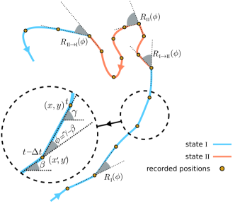
Figure 1: Sketch of a sample trajectory with two states of motion. The selected directional changes along the trajectory represent the four possible turning angles introduced in the model: the directional changes within the states (characterized by the turning-angle distributions $R_{{}_{\text{I}}}\!(\phi)$ and $R_{{}_{\text{I\!I}}}\!(\phi)$) and the changes in the direction of motion at the switching events (characterized by the turning-angle distributions $R_{{}_{\text{I}\rightarrow\text{I\!I}}}\!(\phi)$ and $R_{{}_{\text{I\!I}\rightarrow\text{I}}}\!(\phi)$). The inset magnifies the trajectory around the successive timesteps $t{-}\Delta t$ and $t$. After a change $\phi\,{=}\,\gamma\,{-}\,\beta$ in the direction of motion at $t{-}\Delta t$, the particle arrives at position $(x,y)$ along the direction $\gamma$ at time $t$.

For generality, we assume that the particle moves with a variable instantaneous velocity. At each timestep, the instantaneous velocity is drawn from an arbitrary velocity distribution $F\!\!_{{}_{\text{I}}}{(v)}$ or $F\!\!_{{}_{\text{I\!I}}}{(v)}$ for state I or I​I of motion, respectively. The n-th velocity moment in the j-th state is given as $\langle v^{\text{n}}\rangle_{{}_{\text{j}}}{=}\int_{0}^{{\infty}}\!v^{\text{n}}\,F\!\!_{{}_{\text{j}}}{(v)}\,\text{d}v$. For the calculation of the MSD presented in the Appendix, the relevant velocity moments are only the mean and the second moment, denoted with $\langle v\rangle_{{}_{\text{I}}}$, $\langle v\rangle_{{}_{\text{I\!I}}}$, $\langle v^{2}\rangle_{{}_{\text{I}}}$, and $\langle v^{2}\rangle_{{}_{\text{I\!I}}}$. However, higher velocity moments also appear in the calculation of higher displacement moments as well as other transport quantities of interest.

We introduce four turning-angle distributions for the directional change $\phi$ of the particle between successive time points of the random walk Shaebani et al. (2014); Burov et al. (2013): $R_{{}_{\text{I}}}\!(\phi)$ and $R_{{}_{\text{I\!I}}}\!(\phi)$ for turning events within the states and $R_{{}_{\text{I}\rightarrow\text{I\!I}}}\!(\phi)$ and $R_{{}_{\text{I\!I}\rightarrow\text{I}}}\!(\phi)$ for changing the direction of motion when switching between the states (see Fig. 1). We quantify the persistence in each state by

$$a_{{}_{\text{I}}} \;{=}\!\displaystyle\int_{-{\pi}}^{{\pi}}\!\!\!\!e^{i\phi}\,R_{\text{I}}(\phi)\;\text{d}\phi,$$

$$a_{{}_{\text{I\!I}}} \;{=}\!\displaystyle\int_{-{\pi}}^{{\pi}}\!\!\!\!e^{i\phi}\,R_{\text{I\!I}}(\phi)\;\text{d}\phi.$$ (1)

In many applications, turning-angle distributions are symmetric and the persistencies reduce to real numbers $a_{{}_{\text{I}}}\,{=}\,\langle\cos\phi\rangle\!_{{}_{R_{\text{I}}}}$ and $a_{{}_{\text{I\!I}}}\,{=}\,\langle\cos\phi\rangle\!_{{}_{R_{\text{I\!I}}}}$ in the interval $[-1,1]$. According to this generalized definition of the persistence, one obtains a positive $a_{{}_{\text{j}}}$ if $R_{{}_{\text{j}}}\!(\phi)$ is peaked around forward directions (persistent random walk). An isotropic $R_{{}_{\text{j}}}\!(\phi)$ leads to $a_{{}_{\text{j}}}{=}\,0$ (diffusion) and a distribution which is peaked around backward directions leads to a negative $a_{{}_{\text{j}}}$ (anti-persistent random walk). The extreme values $a_{{}_{\text{j}}}{=}\,{+}1$ and ${-}1$ correspond to a ballistic motion and a pure localization, respectively. For the general case of an asymmetric $R_{{}_{\text{j}}}\!(\phi)$, $a_{{}_{\text{j}}}$ has a nonzero imaginary part in the absence of the left-right symmetry ($a_{{}_{\text{j}}}{=}\,\langle\cos\phi\rangle\!_{{}_{R_{\text{j}}}}{\pm}\,i\,\langle\sin\phi\rangle\!_{{}_{R_{\text{j}}}}$) which leads to a spiral trajectory Sadjadi et al. (2015) (as observed, e.g., for the dynamics of E. coli near surfaces Perez Ipina et al. (2019)).

The particle switches stochastically between the two states with asymmetric probabilities $f\!_{{}_{\text{I}\rightarrow\text{I\!I}}}$ and $f\!_{{}_{\text{I\!I}\rightarrow\text{I}}}$. Assuming constant transition probabilities $f\!_{{}_{\text{I}\rightarrow\text{I\!I}}}$ and $f\!_{{}_{\text{I\!I}\rightarrow\text{I}}}$ leads to exponential residence time distributions

$$F\!\!_{{}_{\text{I}}}{(\tau)}{\sim}\,\displaystyle\text{e}^{\ln(1{-}f\!_{{}_{\text{I}\rightarrow\text{I\!I}}}\!)\;\!\tau},\;F\!\!_{{}_{\text{I\!I}}}{(\tau)}{\sim}\,\displaystyle\text{e}^{\ln(1{-}f\!_{{}_{\text{I\!I}\rightarrow\text{I}}}\!)\;\!\tau},$$ (2)

with the mean residence times

$$\langle\tau\rangle_{{}_{\text{I}}}{=}1{/}f\!_{{}_{\text{I}\rightarrow\text{I\!I}}},\;\langle\tau\rangle_{{}_{\text{I\!I}}}{=}1{/}f\!_{{}_{\text{I\!I}\rightarrow\text{I}}}.$$ (3)

For non-exponential residence-time distributions see e.g. Sadjadi and Shaebani (2021); Detcheverry (2017). For generality, we assume that each switching event is accompanied by a change in the direction of motion according to the turning-angle distribution $R_{{}_{\text{I}\rightarrow\text{I\!I}}}\!(\phi)$ or $R_{{}_{\text{I\!I}\rightarrow\text{I}}}\!(\phi)$. Similar to the persistence of each state, the persistence at each state-switching event can be quantified as

$$a_{{}_{\text{I}\rightarrow\text{I\!I}}} \;{=}\!\displaystyle\int_{-{\pi}}^{{\pi}}\!\!\!\!e^{i\phi}\,R_{{}_{\text{I}\rightarrow\text{I\!I}}}\!(\phi)\;\text{d}\phi,$$

$$a_{{}_{\text{I\!I}\rightarrow\text{I}}} \;{=}\!\displaystyle\int_{-{\pi}}^{{\pi}}\!\!\!\!e^{i\phi}\,R_{{}_{\text{I\!I}\rightarrow\text{I}}}\!(\phi)\;\text{d}\phi,$$ (4)

and assuming symmetric distributions $R_{{}_{\text{I}\rightarrow\text{I\!I}}}\!(\phi)$ and $R_{{}_{\text{I\!I}\rightarrow\text{I}}}\!(\phi)$, the above equations reduce to real numbers $a_{{}_{\text{I}\rightarrow\text{I\!I}}}\,{=}\,\langle\cos\phi\rangle\!_{{}_{R_{{}_{\text{I}\rightarrow\text{I\!I}}}}}$ and $a_{{}_{\text{I\!I}\rightarrow\text{I}}}\,{=}\,\langle\cos\phi\rangle\!_{{}_{R_{{}_{\text{I\!I}\rightarrow\text{I}}}}}$. A turning measure $a_{{}_{\text{j}\rightarrow\text{j}^{\prime}}}$ close to 1, -1, or 0 corresponds, respectively, to slightly changing, reversing, or randomizing the direction of motion when switching from state j to $\text{j}^{\prime}$.

III Evolution of the mean square displacement

We introduce $P\!\!_{t}^{\;\,\text{I}}(x,y|\gamma)$ and $P\!\!_{t}^{\;\,\text{I\!I}}(x,y|\gamma)$ for states I and I​I of motion as the joint probability density functions to find the particle at time $t$ at position $(x,y)$ provided that the particle has reached this position along the direction $\gamma$ (see Fig. 1). We assume that a turning angle $\phi\,{=}\,\gamma\,{-}\,\beta$ has occurred after leaving the old position ($x^{\prime}{=}\,x{-}v\Delta t\cos\gamma$, $y^{\prime}{=}\,y{-}v\Delta t\sin\gamma$) at the previous timestep $t{-}\Delta t$. The total probability density $P\!_{t}(x,y|\gamma)$ is then given by $P\!_{t}(x,y|\gamma)\,{=}\,P\!\!_{t}^{\;\,\text{I}}(x,y|\gamma)\,{+}\,P\!\!_{t}^{\;\,\text{I\!I}}(x,y|\gamma)$. The stochastic process sketched in Fig. 1 is described by the Master equation for the probability densities $P\!\!_{t}^{\;\,\text{I}}(x,y|\gamma)$ and $P\!\!_{t}^{\;\,\text{I\!I}}(x,y|\gamma)$:

$$\left(\!\!\begin{array}[]{ccccccccc}P\!\!_{t}^{\;\,\text{I}}(x,y|\gamma)\\ &\\ P\!\!_{t}^{\;\,\text{I\!I}}(x,y|\gamma)\end{array}\!\!\!\!\!\!\right)=\displaystyle\int\!\!\!dv\!\!\!\displaystyle\int_{\!{-}\pi}^{\pi}\!\!\!\!\!\!d\beta\!\!\displaystyle\left[\!\!\!\begin{array}[]{ccccccccc}(1{-}f\!_{{}_{\text{I}\rightarrow\text{I\!I}}}\!)F\!\!_{{}_{\text{I}}}{(v)}R_{{}_{\text{I}}}\!(\gamma{-}\beta)&f\!_{{}_{\text{I\!I}\rightarrow\text{I}}}F\!\!_{{}_{\text{I}}}{(v)}R_{{}_{\text{I\!I}\rightarrow\text{I}}}\!(\gamma{-}\beta)\\ &\\ \!\!\!\!f\!_{{}_{\text{I}\rightarrow\text{I\!I}}}F\!\!_{{}_{\text{I\!I}}}{(v)}R_{{}_{\text{I}\rightarrow\text{I\!I}}}\!(\gamma{-}\beta)&\!\!\!\!(1{-}f\!_{{}_{\text{I\!I}\rightarrow\text{I}}}\!)F\!\!_{{}_{\text{I\!I}}}{(v)}R_{{}_{\text{I\!I}}}\!(\gamma{-}\beta)\end{array}\!\!\!\right]\,\left(\!\!\begin{array}[]{ccccccccc}P\!\!_{t{-}\Delta t}^{\;\,\text{I}}(x^{\prime},y^{\prime}|\beta)\\ &\\ P\!\!_{t{-}\Delta t}^{\;\,\text{I\!I}}(x^{\prime},y^{\prime}|\beta)\end{array}\!\!\!\!\!\!\right).$$ (14)

Each of the master equations consists of two terms on the right hand side, which represent the possibility of being in each of the two states in the previous time step. The change in the direction of motion $\phi{=}\gamma{-}\beta$ is randomly chosen from the four turning-angle distributions. Here, the velocity and turning-angle distributions are independent but they can be correlated in general Shaebani et al. (2020); Cherstvy et al. (2018). Also, successive velocities are assumed to be uncorrelated for simplicity but they can be correlated in general. In such a case, $F(v)$ can be replaced with a velocity-change distribution similar to $R(\gamma\,{-}\,\beta)$. This would lead to a convolution form after Fourier transform, which cannot be solved in the general form. However, it is possible to solve the problem for at least some explicit forms of the velocity-change distribution. Using the Fourier transform of the probability density function

$$\mathcal{\widetilde{P}}_{t}({\bm{k}}|m)\,{=}\!\!\int\limits_{-\pi}^{\;\;\pi}\!\!\text{d}\gamma\,e^{im\gamma}\!\!\int\!\!\text{d}y\!\!\int\!\!\text{d}x\,\,e^{i\bm{k}\cdot\bm{r}}P\!_{t}(x,y|\gamma),$$ (15)

the displacement moments can be extracted as

$$\langle x^{a}y^{b}\rangle(t)=(-i)^{a+b}\frac{\partial^{a+b}\mathcal{\widetilde{P}}_{t}(k_{x},k_{y}|m=0)}{\partial k_{x}^{a}\partial k_{y}^{b}}\Big{|}_{(k_{x},k_{y})=(0,0)}.$$ (16)

For example, using the polar representation of $\bm{k}$ as $(k,\alpha)$, the $x$ component of the MSD can be calculated as

$$\langle x^{2}\rangle(t)=(-i)^{2}\frac{\partial^{2}\mathcal{\widetilde{P}}_{\!{}_{t}}(k,\alpha{=}0|m{=}0)}{\partial k^{2}}\Big{|}_{k{=}0}.$$ (17)

We present a Fourier-z-transform technique in the Appendix to obtain analytical expressions for arbitrary displacement moments for the stochastic process described by the master equations (14); see also Sadjadi et al. (2015, 2008). The recipe to obtain an arbitrary displacement moment is provided and the calculations are shown in detail to obtain an exact expression for the time evolution of the MSD, which is of broad interest. The formalism can be extended to extract other transport quantities such as the first-passage properties.

The initial probabilities $q_{{}_{0}}^{\text{I}}$ and $q_{{}_{0}}^{\text{I\!I}}$ of starting in state I or I​I influence the short-time dynamics but after some time the probabilities $q_{{}_{t}}^{\text{I}}$ and $q_{{}_{t}}^{\text{I\!I}}$ eventually converge to their steady state values $q_{\text{steady}}^{\text{I}}$ and $q_{\text{steady}}^{\text{I\!I}}$, that are not only independent of the initial probabilities ($q_{{}_{0}}^{\text{I}},\,q_{{}_{0}}^{\text{I\!I}}$) but also independent of time. Note that the process of being in each state is different from the original process defined by the particle positions and directions. Thus, the steady state of $q_{{}_{t}}^{\text{I}}$ and $q_{{}_{t}}^{\text{I\!I}}$ differs from the long-time diffusive dynamics regime of $P\!\!_{t}(x,y|\gamma)$. To estimate the timescale for reaching the steady state, the sequence of being in state I or I​I can be considered as a restricted Markov chain with transition probabilities $f\!_{{}_{\text{I}\rightarrow\text{I\!I}}}$ and $f\!_{{}_{\text{I\!I}\rightarrow\text{I}}}$. By solving

$$\left(\!\!\begin{array}[]{cc}q_{{}_{t}}^{\text{I}}\\ \\ q_{{}_{t}}^{\text{I\!I}}\end{array}\!\!\right){=}\left(\!\!\begin{array}[]{cc}1{-}f\!_{{}_{\text{I}\rightarrow\text{I\!I}}}\,\,\,\,\,\,f\!_{{}_{\text{I\!I}\rightarrow\text{I}}}\\ \\ \,\,\,f\!_{{}_{\text{I}\rightarrow\text{I\!I}}}\,\,\,\,\,\,1{-}f\!_{{}_{\text{I\!I}\rightarrow\text{I}}}\end{array}\!\!\right)^{\!t}\left(\!\!\begin{array}[]{cc}q_{{}_{0}}^{\text{I}}\\ \\ q_{{}_{0}}^{\text{I\!I}}\end{array}\!\!\right),$$ (18)

it can be verified that the time evolution of the restricted Markov chain follows

$$q_{{}_{t}}^{\text{I}}\, {=}\,\displaystyle\frac{f\!_{{}_{\text{I\!I}\rightarrow\text{I}}}}{f\!_{{}_{\text{I}\rightarrow\text{I\!I}}}{+}f\!_{{}_{\text{I\!I}\rightarrow\text{I}}}}+\displaystyle\frac{(1{-}f\!_{{}_{\text{I\!I}\rightarrow\text{I}}}{-}f\!_{{}_{\text{I}\rightarrow\text{I\!I}}})^{t}}{f\!_{{}_{\text{I}\rightarrow\text{I\!I}}}{+}f\!_{{}_{\text{I\!I}\rightarrow\text{I}}}}(f\!_{{}_{\text{I}\rightarrow\text{I\!I}}}\,q_{{}_{0}}^{\text{I}}{-}f\!_{{}_{\text{I\!I}\rightarrow\text{I}}}\,q_{{}_{0}}^{\text{I\!I}}),$$

$$q_{{}_{t}}^{\text{I\!I}}\, {=}\,\displaystyle\frac{f\!_{{}_{\text{I}\rightarrow\text{I\!I}}}}{f\!_{{}_{\text{I}\rightarrow\text{I\!I}}}{+}f\!_{{}_{\text{I\!I}\rightarrow\text{I}}}}+\displaystyle\frac{(1{-}f\!_{{}_{\text{I\!I}\rightarrow\text{I}}}{-}f\!_{{}_{\text{I}\rightarrow\text{I\!I}}})^{t}}{f\!_{{}_{\text{I}\rightarrow\text{I\!I}}}{+}f\!_{{}_{\text{I\!I}\rightarrow\text{I}}}}(f\!_{{}_{\text{I\!I}\rightarrow\text{I}}}\,q_{{}_{0}}^{\text{I\!I}}{-}f\!_{{}_{\text{I}\rightarrow\text{I\!I}}}\,q_{{}_{0}}^{\text{I}}).$$

Thus, the restricted Markov process described by the transitions between state I and I​I exponentially approaches the steady state probabilities

$$q_{\text{steady}}^{\text{I}}=\displaystyle\frac{f\!_{{}_{\text{I\!I}\rightarrow\text{I}}}}{f\!_{{}_{\text{I}\rightarrow\text{I\!I}}}{+}f\!_{{}_{\text{I\!I}\rightarrow\text{I}}}},\;q_{\text{steady}}^{\text{I\!I}}=\displaystyle\frac{f\!_{{}_{\text{I}\rightarrow\text{I\!I}}}}{f\!_{{}_{\text{I}\rightarrow\text{I\!I}}}{+}f\!_{{}_{\text{I\!I}\rightarrow\text{I}}}}.$$ (20)

If the process initially starts with the steady state probabilities, i.e. $q_{{}_{0}}^{\text{I}}\,{=}\,q_{\text{steady}}^{\text{I}}$ and $q_{{}_{0}}^{\text{I\!I}}\,{=}\,q_{\text{steady}}^{\text{I\!I}}$, the last parentheses on the right hand side of Eqs. (LABEL:Eq:Markov_Evolve) will be zero and the restricted Markov process is immediately in the steady state. Similarly, for the specific choice of $f\!_{{}_{\text{I}\rightarrow\text{I\!I}}}\,{+}\,f\!_{{}_{\text{I\!I}\rightarrow\text{I}}}\,{=}\,1$, the exponential terms on the right hand side of Eqs. (LABEL:Eq:Markov_Evolve) will be zero and again the the restricted Markov process is immediately in the steady state. The characteristic time to exponentially approach the steady state can be obtained from Eqs. (LABEL:Eq:Markov_Evolve) as

$$t_{\text{s}}=\displaystyle\frac{-1}{\ln|1{-}f\!_{{}_{\text{I}\rightarrow\text{I\!I}}}{-}f\!_{{}_{\text{I\!I}\rightarrow\text{I}}}|}\,.$$ (21)

By choosing steady state initial conditions— i.e. $q_{{}_{0}}^{\text{I}}\,{=}\,q_{\text{steady}}^{\text{I}}$ and $q_{{}_{0}}^{\text{I\!I}}\,{=}\,q_{\text{steady}}^{\text{I\!I}}$—, we exclude the role of the initial conditions and reduce the complexity of the short-time dynamics. For this choice and an isotropic initial orientation, after some calculations (see Appendix) we obtain the following exact expression for the time evolution of the MSD

$$\langle r^{2}\rangle(t)=\mathcal{A}+\mathcal{B}\,t+\mathcal{C}\,\text{e}^{-t{/}t_{\text{c}_{+}}}+\mathcal{D}\,\text{e}^{-t{/}t_{\text{c}_{-}}},$$ (22)

with characteristic times

$$t_{\text{c}_{\pm}}{=}\displaystyle\frac{-1}{\ln\Bigg{|}\frac{a_{{}_{\text{I}}}(1{-}f\!_{{}_{\text{I}\rightarrow\text{I\!I}}})\,{+}\,a_{{}_{\text{I\!I}}}(1{-}f\!_{{}_{\text{I\!I}\rightarrow\text{I}}}){\pm}\sqrt{\big{(}a_{{}_{\text{I}}}(1{-}f\!_{{}_{\text{I}\rightarrow\text{I\!I}}})\,{-}\,a_{{}_{\text{I\!I}}}(1{-}f\!_{{}_{\text{I\!I}\rightarrow\text{I}}})\big{)}^{2}\!{+}\,4\,a_{{}_{\text{I}\rightarrow\text{I\!I}}}\,a_{{}_{\text{I\!I}\rightarrow\text{I}}}\,f\!_{{}_{\text{I}\rightarrow\text{I\!I}}}\,f\!_{{}_{\text{I\!I}\rightarrow\text{I}}}}}{2}\Bigg{|}},$$ (23)

which reduces to $t_{\text{c}}{=}\frac{-1}{\ln|a|}$ for a single-state persistent random walk (i.e. for $f\!_{{}_{\text{I}\rightarrow\text{I\!I}}}{=}0$ and $f\!_{{}_{\text{I\!I}\rightarrow\text{I}}}{=}1$) with persistence $a$. The time-independent term $\mathcal{A}$ and the prefactors $\mathcal{B}$, $\mathcal{C}$ and $\mathcal{D}$ are functions of the persistencies ($a_{{}_{\text{I}}}$, $a_{{}_{\text{I\!I}}}$, $a_{{}_{\text{I}\rightarrow\text{I\!I}}}$, $a_{{}_{\text{I\!I}\rightarrow\text{I}}}$), the switching probabilities ($f\!_{{}_{\text{I}\rightarrow\text{I\!I}}}$, $f\!_{{}_{\text{I\!I}\rightarrow\text{I}}}$), and the first two velocity moments ($\langle v\rangle_{{}_{\text{I}}}$, $\langle v\rangle_{{}_{\text{I\!I}}}$, $\langle v^{2}\rangle_{{}_{\text{I}}}$, $\langle v^{2}\rangle_{{}_{\text{I\!I}}}$); see Appendix. Equation (22) shows that the MSD consists of exponentially-decaying terms with $t$, a time-independent term, and a term which grows linearly with $t$. The short-time dynamics is mainly controlled by the exponentially-decaying and time-independent terms, whereas the linear term dominates at long times. Note that only the first Fourier mode of each turning-angle distribution (i.e. $\langle\cos\phi\rangle$) appears in the calculation of the MSD and the overall form the distribution plays no role. Higher Fourier modes of the turning-angle distribution appear in the calculation of the higher displacement moments. For example, $\langle\cos(2\phi)\rangle$ appears in the expression for $\langle r^{4}\rangle(t)$ Sadjadi et al. (2015). Although Eq. (22) is a profitable expression to compare with the experimental data, we advise (especially for non-steady state initial conditions) to insert the parameter values into the much shorter form of the MSD before the inverse z-transform, i.e. $\langle r^{2}\rangle(z)$ given in Eq. (65), and then use Mathematica or any other software to apply the inverse z-transform and obtain the analytical form of the MSD as a function of $t$.

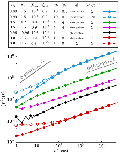
Figure 2: Time evolution of the MSD in log-log scale. The symbols denote simulation results and the lines correspond to analytical predictions via Eq. (22). A rich variety of dynamical regimes of anomalous motion can be observed at short and intermediate time scales. The velocity of each state is constant except for the blue (upper) dashed curve, which is obtained for broad uniform velocity distributions (with $\langle v^{2}\rangle\,{=}\,20\,\langle v\rangle^{2}$ in both states). All the MSD profiles belong to steady state initial conditions except for the red (lower) dashed curve which is obtained for the initial condition $q_{{}_{0}}^{\text{I}}\,{=}\,1$, i.e. starting the motion in state I. In all plots we have chosen $a_{{}_{\text{I}\rightarrow\text{I\!I}}}\,{=}\,a_{{}_{\text{I\!I}}}$ and $a_{{}_{\text{I\!I}\rightarrow\text{I}}}\,{=}\,a_{{}_{\text{I}}}$ for the directional changes at the switching events. An ensemble of $10^{5}$ realizations has been considered for the simulations and the four turning-angle distributions are uniformly distributed around the zero change in the turning angle.

Figure 2 shows the time evolution of MSD over a wide range of time scales. Various types of anomalous diffusion (i.e. MSD $\langle r^{2}\rangle(t)$ not proportional to $t$) can be observed upon varying the key parameters. For simplicity, we have presented the results for $a_{{}_{\text{I}\rightarrow\text{I\!I}}}\,{=}\,a_{{}_{\text{I\!I}}}$ and $a_{{}_{\text{I\!I}\rightarrow\text{I}}}\,{=}\,a_{{}_{\text{I}}}$ at the switching events, a constant velocity in each state, and steady state initial conditions (solid lines and symbols), unless specified otherwise. For visibility, different velocity values are used to separate the curves from each other. The shape of the MSD profile strongly depends on the choice of persistence parameters and switching probabilities. For a combination of two persistent random walks, the crossover from the initial superdiffusive to the asymptotic diffusive dynamics can be delayed by increasing the persistencies or the residence time in the more persistent state. A mixture of a persistent and a slightly antipersistent walk results in a subdiffusive dynamics at short times. However, by choosing a strongly antipersistent state, an oscillatory dynamics at short timescales emerges Tierno et al. (2012); Tierno and Shaebani (2016). In some parameter regimes, the exponential terms of the MSD rapidly decay and time-independent terms develop a plateau regime over intermediate timescales; see, e.g., the red (lower) dashed curve obtained by choosing $q_{{}_{0}}^{\text{I}}\,{=}\,1$ instead of steady state initial conditions. The initial conditions influence the time-independent and exponentially-decaying terms of the MSD and diversify the anomalous diffusion on short time scales. However, the term which grows linearly with $t$ is independent of the initial conditions, thus, the profiles for different initial conditions eventually merge at long times when the crossover to asymptotic diffusive dynamics occurs.

We have presented the formalism in the Appendix for an arbitrary choice of the initial condition until Eq. (65) for the MSD in the z-space but then solved the inverse z-transform problem for the specific choice of steady state initial conditions. Thus, by inserting any desired initial condition into Eq. (65) and calculating the inverse z-transform, the time evolution of MSD can be obtained (as we did for the red (lower) dashed curve in Fig. 2).

To see how the velocity variations influence the MSD profile, we present an example of variable velocities in Fig. 2 (blue (upper) dashed curve): A wide velocity distribution in each state is chosen ($\langle v^{2}\rangle_{{}_{\text{I}}}\,{=}\,20\,\langle v\rangle^{2}_{{}_{\text{I}}}$ and $\langle v^{2}\rangle_{{}_{\text{I\!I}}}\,{=}\,20\,\langle v\rangle^{2}_{{}_{\text{I\!I}}}$). It can be seen that the broadening of the velocity distributions unexpectedly pushes the initial slope towards the diffusion line by increasing the role of the linear term of the MSD.

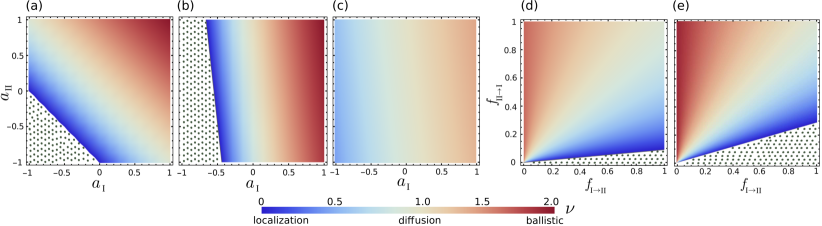
Figure 3: Phase diagrams of the initial anomalous exponent according to Eq. (25). The color intensity reflects the magnitude of $\nu$, with red (blue) meaning superdiffusion (subdiffusion). The dotted regions denote oscillatory subdomains. We consider $a_{{}_{\text{I}\rightarrow\text{I\!I}}}\,{=}\,a_{{}_{\text{I\!I}}}$ and $a_{{}_{\text{I\!I}\rightarrow\text{I}}}\,{=}\,a_{{}_{\text{I}}}$ in all panels and choose a constant velocity ($\langle v\rangle\,{=}\,\langle v^{2}\rangle\,{=}\,1$) in both states, except for panel (c). (a, b) $\nu$ in $(a_{{}_{\text{I}}},a_{{}_{\text{I\!I}}})$ plane for (a) $f\!_{{}_{\text{I}\rightarrow\text{I\!I}}}\,{=}\,f\!_{{}_{\text{I\!I}\rightarrow\text{I}}}\,{=}\,0.5$ and (b) $f\!_{{}_{\text{I}\rightarrow\text{I\!I}}}\,{=}\,0.1$, $f\!_{{}_{\text{I\!I}\rightarrow\text{I}}}\,{=}\,0.9$. By the asymmetric choices of $f\!_{{}_{\text{I}\rightarrow\text{I\!I}}}$ and $f\!_{{}_{\text{I\!I}\rightarrow\text{I}}}$, $\nu$ is influenced stronger by the persistence of the state with a longer mean residence time. (c) Similar parameter values as in panel (b) but with broad velocity distributions ($\langle v\rangle\,{=}\,1$ and $\langle v^{2}\rangle\,{=}\,3$ in both states). Broader velocity distributions push the initial slope of the MSD towards $\nu\,{=}\,1$ (diffusion). (d, e) $\nu$ in $(f\!_{{}_{\text{I}\rightarrow\text{I\!I}}},f\!_{{}_{\text{I\!I}\rightarrow\text{I}}})$ plane for a combination of persistent and antipersistent motions characterized by (d) $a_{{}_{\text{I}}}\,{=}\,0.6$, $a_{{}_{\text{I\!I}}}\,{=}\,-0.6$ and (e) $a_{{}_{\text{I}}}\,{=}\,0.9$, $a_{{}_{\text{I\!I}}}\,{=}\,-0.9$. $\nu$ is enhanced by the switching probabilities that lead to a longer stay in the persistent mode.

To confirm the validity of the analytical predictions, we perform extensive Monte Carlo simulations of the stochastic process. We consider a 2D persistent random walk with two different modes of motion and allow the walker to spontaneously change the mode of motion at each timestep according to given asymmetric transition probabilities. By choosing an arbitrary length unit, the step size has been varied within the range [0.01, 100] depending on the choice of the velocity distributions. Periodic boundary conditions are imposed and the results are shown for the system size $L\,{=}\,10^{5}$. The walker starts at the center of the simulation box and the initial orientation of motion is randomly drawn from an isotropic distribution. For the velocity and turning-angle distributions, we have chosen uniform distributions which are symmetric around the mean velocity of each state or the turning angle $\phi\,{=}\,0$, respectively. However, we note that choosing other arbitrary distributions with the same first two velocity moments and mean persistence $\langle\cos\phi\rangle$ lead to exactly the same MSD profile (though, higher displacement moments would differ from those of the uniform distribution choice). Figure 2 shows the simulation results, averaged over an ensemble of $10^{5}$ realizations. The simulation results agree perfectly with the analytical predictions.

IV Initial anomalous exponent

The transient dynamics is of particular interest as the time window of experiments is practically limited. To characterize and compare the initial growth rate of the MSD profiles, one can assign an initial anomalous exponent to each MSD curve by fitting it to a power-law $\langle r^{2}\rangle(t){\sim}t^{\nu}$. To this aim, we obtain the MSD of the first two points along the curve from Eq. (22) as $\langle r^{2}\rangle(t{=}1)\,{=}\,\mathcal{A}\,{+}\,\mathcal{B}\,{+}\,\mathcal{C}\,\text{e}^{-1{/}t_{\text{c}_{+}}}+\mathcal{D}\,\text{e}^{-1{/}t_{\text{c}_{-}}}$ and $\langle r^{2}\rangle(t{=}2)\,{=}\,\mathcal{A}\,{+}\,2\,\mathcal{B}\,{+}\,\mathcal{C}\,\text{e}^{-2{/}t_{\text{c}_{+}}}+\mathcal{D}\,\text{e}^{-2{/}t_{\text{c}_{-}}}$. The power-law fit passes both of these points leading to $\ln\,\langle r^{2}\rangle(t{=}2)-\ln\,\langle r^{2}\rangle(t{=}1)=\nu\,(\ln 2-\ln 1)$, from which the initial anomalous exponent can be obtained as

$$\nu=\ln\Big{(}\displaystyle\frac{\langle r^{2}\rangle(t{=}2)}{\langle r^{2}\rangle(t{=}1)}\Big{)}{\Big{/}}\ln 2.$$ (24)

By replacing the MSD from Eq. (22) and after some algebra, we derive the initial anomalous exponent

$$\nu{=}1{+}\ln\Big{(}\!1{+}\frac{f\!_{{}_{\text{I}\rightarrow\text{I\!I}}}\,f\!_{{}_{\text{I\!I}\rightarrow\text{I}}}\,\langle v\rangle_{{}_{\text{I}}}\,\langle v\rangle_{{}_{\text{I\!I}}}\,(a_{{}_{\text{I}\rightarrow\text{I\!I}}}\,{+}\,a_{{}_{\text{I\!I}\rightarrow\text{I}}})\,{+}\,a_{{}_{\text{I}}}\,\langle v\rangle^{2}_{{}_{\text{I}}}\,(1\,{-}\,f\!_{{}_{\text{I}\rightarrow\text{I\!I}}})\,f\!_{{}_{\text{I\!I}\rightarrow\text{I}}}\,{+}\,a_{{}_{\text{I\!I}}}\,\langle v\rangle^{2}_{{}_{\text{I\!I}}}\,f\!_{{}_{\text{I}\rightarrow\text{I\!I}}}\,(1\,{-}\,f\!_{{}_{\text{I\!I}\rightarrow\text{I}}})}{f\!_{{}_{\text{I}\rightarrow\text{I\!I}}}\,\langle v^{2}\rangle_{{}_{\text{I\!I}}}\,{+}\,f\!_{{}_{\text{I\!I}\rightarrow\text{I}}}\,\langle v^{2}\rangle_{{}_{\text{I}}}}\Big{)}{\Big{/}}\ln 2.$$ (25)

For a single-state active motion (i.e. $f\!_{{}_{\text{I}\rightarrow\text{I\!I}}}{=}0$ and $f\!_{{}_{\text{I\!I}\rightarrow\text{I}}}{=}1$) with persistence $a$ and constant velocity, the above equation reduces to $\nu\,{=}\,1\!+\frac{\ln(1{+}a)}{\ln 2}$ Shaebani et al. (2014). Since all four persistence parameters appear linearly and with similar prefactors, we choose $a_{{}_{\text{I}\rightarrow\text{I\!I}}}\,{=}\,a_{{}_{\text{I\!I}}}$ and $a_{{}_{\text{I\!I}\rightarrow\text{I}}}\,{=}\,a_{{}_{\text{I}}}$ at the switching events for simplicity. In the phase diagrams presented in Fig. 3, we show how $\nu$ depends on the remaining key parameters. $\nu$ ranges from 2 for ballistic motion to 1 for diffusion and 0 for zero net displacement. The onset of oscillatory dynamics for a strongly antipersistent random walk can be identified by setting $\nu\,{=}\,0$. Figure 3(a) shows that $\nu$ varies symmetrically in ($a_{{}_{\text{I}}}$, $a_{{}_{\text{I\!I}}}$) plane for symmetric transitions between the states, i.e. for $f\!_{{}_{\text{I}\rightarrow\text{I\!I}}}\,{=}\,f\!_{{}_{\text{I\!I}\rightarrow\text{I}}}$. However, for an asymmetric choice of the switching probabilities $f\!_{{}_{\text{I}\rightarrow\text{I\!I}}}\,{<}\,f\!_{{}_{\text{I\!I}\rightarrow\text{I}}}$, $\nu$ is more sensitive to the persistence of state I, which has a longer mean residence time according to Eq. (3); see panel (b). Using broad velocity distributions as in panel (c) increases the denominator in Eq. (25) and results in considerably smaller anomalous exponents, which is consistent with the short-time behavior of the MSD in Fig. 2 (blue (upper) dashed curve vs blue (upper) solid curve). For a mixture of persistent ($a_{{}_{\text{I}}}\,{>}\,0$) and antipersistent ($a_{{}_{\text{I\!I}}}\,{<}\,0$) states in panel (d), the combination of switching probabilities that increases the residence time in the persistent state (i.e. a smaller $f\!_{{}_{\text{I}\rightarrow\text{I\!I}}}$ and a larger $f\!_{{}_{\text{I\!I}\rightarrow\text{I}}}$) enhances the anomalous exponent. The effect becomes stronger with increasing the magnitude of the persistencies $a_{{}_{\text{I}}}$ and $a_{{}_{\text{I\!I}}}$ in panel (e).

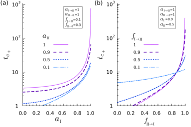
Figure 4: Characteristic time $t_{\text{c}_{+}}$ via Eq. (23) in terms of (a) $a_{{}_{\text{I}}}$ and (b) $f\!_{{}_{\text{I\!I}\rightarrow\text{I}}}$. The switching persistencies are chosen as $a_{{}_{\text{I}\rightarrow\text{I\!I}}}\,{=}\,a_{{}_{\text{I\!I}\rightarrow\text{I}}}\,{=}\,1$ in both panels. The crossover time grows by several orders of magnitude by increasing the persistence of the states or increasing the residence time in the more persistent mode. In panel (a), the results for several values of $a_{{}_{\text{I\!I}}}$ are shown at a given set of $f\!_{{}_{\text{I}\rightarrow\text{I\!I}}}$ and $f\!_{{}_{\text{I\!I}\rightarrow\text{I}}}$ parameters. In panel (b), $a_{{}_{\text{I}}}$ and $a_{{}_{\text{I\!I}}}$ are fixed and $t_{\text{c}_{+}}$ is shown vs $f\!_{{}_{\text{I\!I}\rightarrow\text{I}}}$ for several values of $f\!_{{}_{\text{I}\rightarrow\text{I\!I}}}$.

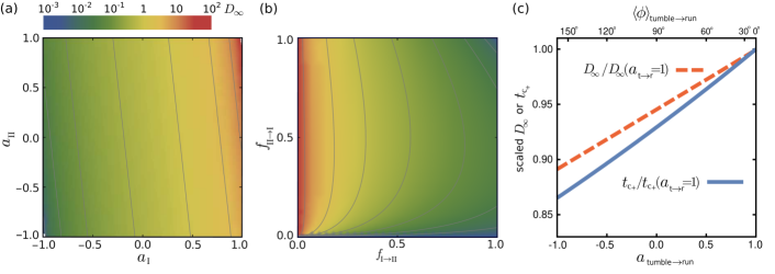
Figure 5: (a),(b) $D\!_{{}_{\infty}}$ in $(a_{{}_{\text{I}}},a_{{}_{\text{I\!I}}})$ and $(f\!_{{}_{\text{I}\rightarrow\text{I\!I}}},f\!_{{}_{\text{I\!I}\rightarrow\text{I}}})$ planes, scaled by $v^{2}\Delta t$, for a constant velocity $v_{{}_{\text{I}}}{=}v_{{}_{\text{I\!I}}}{=}v$ and the parameter values (unless varied): $f\!_{{}_{\text{I}\rightarrow\text{I\!I}}}{=}0.1$, $f\!_{{}_{\text{I\!I}\rightarrow\text{I}}}{=}0.9$, $a_{{}_{\text{I}}}{=}0.9$, $a_{{}_{\text{I\!I}}}{=}-0.9$, $a_{{}_{\text{I\!I}\rightarrow\text{I}}}{=}a_{{}_{\text{I}}}$, $a_{{}_{\text{I}\rightarrow\text{I\!I}}}{=}a_{{}_{\text{I\!I}}}$. By the chosen asymmetric switching probabilities in panel (a), the walker spends longer times in state I and $D\!_{{}_{\infty}}$ is more sensitive to $a_{{}_{\text{I}}}$. Panel (b) shows that tuning the residence time in each state via $f\!_{{}_{\text{I}\rightarrow\text{I\!I}}}$ and $f\!_{{}_{\text{I\!I}\rightarrow\text{I}}}$ in a combination of persistent and antipersistent motions dramatically influences $D\!_{{}_{\infty}}$. (c) Variations of $D\!_{{}_{\infty}}$ and $t_{\text{c}_{+}}$ in a run-and-tumble process in terms of the mean tumble-to-run turning angle $\langle\phi\rangle_{\text{tumble}{\rightarrow}\text{run}}$ (correspondingly $a_{{}_{\text{tumble}\rightarrow\text{run}}}{=}\langle\cos\phi\rangle_{{}_{\text{tumble}\rightarrow\text{run}}}$). Other parameter values: $f\!_{{}_{\text{run}\rightarrow\text{tumble}}}{=}f\!_{{}_{\text{tumble}\rightarrow\text{run}}}{=}0.1$, $a_{{}_{\text{run}}}{=}0.9$, $a_{{}_{\text{tumble}}}{=}0$, $a_{{}_{\text{run}\rightarrow\text{tumble}}}{=}1$, and constant velocities $v_{{}_{\text{run}}}{=}2\,v_{{}_{\text{tumble}}}$.

V Crossover time to asymptotic normal diffusion

Asymptotically the stochastic process considered here is described by normal diffusion (i.e. a non-persistent motion) since it gradually loses its memory of the initial direction and state of motion, and the trajectory eventually gets randomized. It can be seen from Eq. (22) that while the contribution of the term linear in $t$ dominates at large times, the exponential terms decay. To estimate the crossover time to the asymptotic diffusive regime one can, e.g., measure the instantaneous anomalous exponent (similar to the procedure explained in the previous section for the calculation of the initial anomalous exponent $\nu$) and follow its convergence towards 1. Alternatively, the characteristic times of the exponentially-decaying terms of the MSD (i.e. $t_{\text{c}_{+}}$ and $t_{\text{c}_{-}}$) reflect the timescale to approach the long-term dynamics. We follow the later choice and use Eq. (23) to show how the crossover time depends on the key parameters of the particle dynamics. Both $t_{\text{c}_{+}}$ and $t_{\text{c}_{-}}$ depend on the four persistencies $a_{{}_{\text{I}}}$, $a_{{}_{\text{I\!I}}}$, $a_{{}_{\text{I}\rightarrow\text{I\!I}}}$, and $a_{{}_{\text{I\!I}\rightarrow\text{I}}}$ and the switching probabilities $f\!_{{}_{\text{I}\rightarrow\text{I\!I}}}$ and $f\!_{{}_{\text{I\!I}\rightarrow\text{I}}}$ but are independent of the initial conditions and the velocity distributions.

To reduce the degrees of freedom, we set $a_{{}_{\text{I}\rightarrow\text{I\!I}}}=a_{{}_{\text{I\!I}\rightarrow\text{I}}}=1$ (corresponding to move straight forward at the switching events). Figure 4 shows the behavior of $t_{\text{c}_{+}}$, as an example. Similar results can be deduced for $t_{\text{c}_{-}}$ as well. The characteristic time can vary by several orders of magnitude upon changing the remaining control parameters. For a given set of ($f\!_{{}_{\text{I}\rightarrow\text{I\!I}}}$, $f\!_{{}_{\text{I\!I}\rightarrow\text{I}}}$) and a combination of two persistent random walks, it is shown in Fig. 4(a) that $t_{\text{c}_{+}}$ grows with increasing $a_{{}_{\text{I}}}$ and $a_{{}_{\text{I\!I}}}$. For a mixture of persistent $a_{{}_{\text{I}}}$ and antipersistent $a_{{}_{\text{I\!I}}}$ states, Fig. 4(b) reveals that the switching probabilities that lead to a longer residence in the persistent mode (i.e. a larger $f\!_{{}_{\text{I\!I}\rightarrow\text{I}}}$ or a smaller $f\!_{{}_{\text{I}\rightarrow\text{I\!I}}}$) enhance $t_{\text{c}_{+}}$ even by orders of magnitude. We note that the velocity moments may also influence the crossover time through the prefactors $\mathcal{C}$ and $\mathcal{D}$ in Eq. (22).

VI Asymptotic diffusion constant

According to Eq. (22), the exponential terms of the MSD gradually decay and the time-independent term also becomes negligible compared to the linear term at long times. As the linear term eventually dominates, the process is asymptotically diffusive and the MSD follows $\langle r^{2}\rangle(t{\rightarrow}\infty)\,{\sim}\,\mathcal{B}\,t$. By writing the MSD in the diffusion regime as $\langle r^{2}\rangle(t{\rightarrow}\infty)\,{=}\,2\,d\,D\!_{{}_{\infty}}t$ (with $d\,{=}\,2$ being the dimension of the system), the long-term diffusion coefficient can be deduced as

$$D\!_{{}_{\infty}}{=} \frac{\Delta t}{4}\frac{f\!_{{}_{\text{I\!I}\rightarrow\text{I}}}(e_{{}_{2}}{-}1)\langle v^{2}\rangle_{{}_{\text{I}}}{+}f\!_{{}_{\text{I}\rightarrow\text{I\!I}}}(e_{{}_{1}}{-}1)\langle v^{2}\rangle_{{}_{\text{I\!I}}}{-}2\,e_{{}_{4}}\langle v\rangle_{{}_{\text{I}}}\langle v\rangle_{{}_{\text{I\!I}}}{-}f\!_{{}_{\text{I\!I}\rightarrow\text{I}}}\big{(}(e_{{}_{2}}{-}1)e_{{}_{1}}{-}e_{{}_{3}}\big{)}\Delta\,v_{{}_{\text{I}}}{-}f\!_{{}_{\text{I}\rightarrow\text{I\!I}}}\big{(}(e_{{}_{1}}{-}1)e_{{}_{2}}{-}e_{{}_{3}}\big{)}\Delta\,v_{{}_{\text{I\!I}}}}{(f\!_{{}_{\text{I}\rightarrow\text{I\!I}}}{+}f\!_{{}_{\text{I\!I}\rightarrow\text{I}}})\,\Big{(}e_{{}_{3}}\,{-}\,(e_{{}_{1}}{-}1)(e_{{}_{2}}{-}1)\Big{)}},$$ (26)

with $\Delta v_{{}_{\text{j}}}{=}\langle v^{2}\rangle_{{}_{\text{j}}}{-}2\langle v\rangle_{{}_{\text{j}}}^{2}$, $e_{{}_{1}}{=}(1{-}f\!_{{}_{\text{I}\rightarrow\text{I\!I}}})a_{{}_{\text{I}}}$, $e_{{}_{2}}{=}(1{-}f\!_{{}_{\text{I\!I}\rightarrow\text{I}}})a_{{}_{\text{I\!I}}}$, $e_{{}_{3}}{=}f\!_{{}_{\text{I}\rightarrow\text{I\!I}}}f\!_{{}_{\text{I\!I}\rightarrow\text{I}}}a_{{}_{\text{I}\rightarrow\text{I\!I}}}a_{{}_{\text{I\!I}\rightarrow\text{I}}}$, and $e_{{}_{4}}{=}f\!_{{}_{\text{I}\rightarrow\text{I\!I}}}f\!_{{}_{\text{I\!I}\rightarrow\text{I}}}(a_{{}_{\text{I}\rightarrow\text{I\!I}}}{+}a_{{}_{\text{I\!I}\rightarrow\text{I}}})$. For a single-state persistent random walk (i.e. $f\!_{{}_{\text{I}\rightarrow\text{I\!I}}}{=}0$ and $f\!_{{}_{\text{I\!I}\rightarrow\text{I}}}{=}1$) with persistency $a$, the above equation reduces to $D\!_{{}_{\infty}}{=}\frac{\Delta t}{4}\big{(}\langle v^{2}\rangle{+}\frac{2\,a}{1{-}a}\langle v\rangle^{2}\big{)}$ Shaebani et al. (2014).

To visualize $D\!_{{}_{\infty}}$ in terms of the key parameters, we consider a process in which $a_{{}_{\text{I\!I}\rightarrow\text{I}}}{=}a_{{}_{\text{I}}}$ and $a_{{}_{\text{I}\rightarrow\text{I\!I}}}{=}a_{{}_{\text{I\!I}}}$ at the switching events. As shown in Figs. 5(a),(b), $D\!_{{}_{\infty}}$ varies by several orders of magnitude by changing the key parameters ($a_{{}_{\text{I}}}$, $a_{{}_{\text{I\!I}}}$) or ($f\!_{{}_{\text{I}\rightarrow\text{I\!I}}}$, $f\!_{{}_{\text{I\!I}\rightarrow\text{I}}}$). Equation (26) describes $D\!_{{}_{\infty}}$ for any arbitrary combination of the stochastic processes. For instance, for a simple combination of diffusion (with constant $D_{{}_{\text{I}}}$) and waiting, Eq. (26) reduces to $D\!_{{}_{\infty}}{=}D_{{}_{\text{I}}}\displaystyle\frac{f\!_{{}_{\text{I\!I}\rightarrow\text{I}}}}{f\!_{{}_{\text{I}\rightarrow\text{I\!I}}}{+}f\!_{{}_{\text{I\!I}\rightarrow\text{I}}}}$, which was originally shown by Lennard-Jones for surface diffusion with traps Lennard-Jones (1932). $D\!_{{}_{\infty}}$ is independent of the initial conditions $q_{{}_{0}}^{\text{I}}$ and $q_{{}_{0}}^{\text{I\!I}}$, implying that the history of the process is only carried by exponential and time-independent terms of the MSD that are negligible at long times as the linear term eventually dominates.

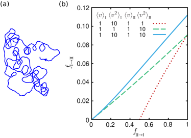
Figure 6: (a) Typical trajectory of a single-state persistent walker with an asymmetric turning-angle distribution uniformly distributed over the range $\phi\,{\in}\,[{-}\frac{\pi}{6},\frac{2\pi}{6}]$. The asymmetry of the turning angles leads to a trajectory with frequent clockwise spirals. The resulting persistence parameter has real and imaginary parts $a_{\text{R}}\,{\simeq}0.9$ and $a_{\text{I}}\,{\simeq}0.2$, respectively. (b) Subset of optimal switching probabilities $f\!_{{}_{\text{I}\rightarrow\text{I\!I}}}^{\,\,\text{opt}}$ and $f\!_{{}_{\text{I\!I}\rightarrow\text{I}}}^{\,\,\text{opt}}$ that maximize the asymptotic diffusion constant according to Eqs. (29) and (30) in the ($f\!_{{}_{\text{I}\rightarrow\text{I\!I}}},f\!_{{}_{\text{I\!I}\rightarrow\text{I}}}$) plane for various choices of the velocity moments in a combination of ballistic and diffusive processes.

VII Applications and special cases

The broad applicability of our formalism allows generic predictions about the dynamics of various systems. In this section we present a few applications and the reduced form of the general analytical expressions for a couple of specific choices for the states of motion.

Bacterial dynamics— Bacterial species that swim by the rotation of flagella experience an alternating sequence of run and tumble phases. An abrupt directional change often occurs when switching back from tumble to run phase Berg (2004); Najafi et al. (2018), which is caused by the torque exerted on the cell body during the reformation of the bundle Darnton et al. (2007). It is hypothesized that the bacteria benefit from this feature to slow their spreading and explore the local environment more precisely. Since in our model the statistics of the turning angles at the switching events are chosen to be independent from the turning angles within the states in general, we can directly check how directional changes at the switching events influence the crossover time to the long-term diffusive dynamics and the asymptotic diffusion coefficient. Figure 5(c) shows that increasing the mean directional change at switching from tumble to run, $\langle\phi\rangle_{\text{tumble}{\rightarrow}\text{run}}$, helps the bacteria to randomize their path: A stronger kick (i.e. a larger turning angle $\langle\phi\rangle_{\text{tumble}{\rightarrow}\text{run}}$) can reduce the crossover time $t_{\text{c}_{+}}$ and the diffusion coefficient $D\!_{{}_{\infty}}$ by more than $10\%$ for the given set of parameters in Fig. 5(c); for a higher run persistence $a_{{}_{\text{run}}}{=}\,0.96$, the percentage of reduction can even exceed $25\%$.

Spiral trajectories— The turning-angle distributions $R_{\text{I}}(\phi)$, $R_{\text{I\!I}}(\phi)$, $R_{{}_{\text{I}\rightarrow\text{I\!I}}}\!(\phi)$ and $R_{{}_{\text{I\!I}\rightarrow\text{I}}}\!(\phi)$ can be asymmetric in general. For any asymmetric distribution $R(\phi)$, the persistence introduced in Eq. (1) or (4) has a real part $a_{{}_{\text{R}}}{=}\int_{-{\pi}}^{{\pi}}\!\text{d}\phi\,\cos\phi\,R(\phi){=}\langle\cos\phi\rangle$ and a nonzero imaginary part $a_{{}_{\text{Im}}}{=}\int_{-{\pi}}^{{\pi}}\!\text{d}\phi\,\sin\phi\,R(\phi){=}\langle\sin\phi\rangle$. If we consider a single-state 2D motion for simplicity, an asymmetric $R(\phi)$ means that the left-right symmetry does not hold and the particle turns more frequently either to the right or to the left direction, leading to the emergence of clockwise or anti-clockwise spiral trajectories. For example, motion with a uniform distribution $R(\phi)\,{=}\,\frac{1}{\pi{/}2}$ but over an asymmetric range $[{-}\frac{\pi}{6},\frac{2\pi}{6}]$ of $\phi$ corresponds to a trajectory with frequent clockwise spirals; see Fig. 6(a). Following the analytical approach presented in the Appendix, one can choose the conditions for a single state (and also set $\alpha{=}m{=}0$ in Eq. (59)) to obtain the expansion coefficient that is required to extract the MSD. Because of the asymmetry of the turning-angle distribution, $\mathcal{\widetilde{R}}(m{=}1){=}a_{{}_{\text{R}}}{+}i\,a_{{}_{\text{Im}}}$ and $\mathcal{\widetilde{R}}(m{=}{-}1){=}a_{{}_{\text{R}}}{-}i\,a_{{}_{\text{Im}}}$, i.e. $\mathcal{\widetilde{R}}(m{=}1){\neq}\mathcal{\widetilde{R}}(m{=}{-}1)$; see Eq. (46). By inserting these quantities into Eq. (59) and following the rest of the procedure, the MSD can be obtained. From the linear term of the MSD in $t$, the asymptotic diffusion constant can be deduced as

$$D\!_{{}_{\infty}}{=}\frac{1}{4}\,v^{2}\!\Delta t\,\frac{a_{{}_{\text{R}}}(1{-}a_{{}_{\text{R}}}){-}a_{{}_{\text{Im}}}^{2}}{(1{-}a_{{}_{\text{R}}}\!)^{2}{+}a_{{}_{\text{Im}}}^{2}},$$ (27)

where we choose a constant velocity $v$ for simplicity. It can be seen that the asymmetric contribution reduces the asymptotic diffusion coefficient. If we denote the diffusion coefficient of a diffusion process ($a_{{}_{\text{R}}}{=}\,a_{{}_{\text{Im}}}{=}\,0$) with $D\!_{{}_{0}}{=}\frac{1}{4}\,v^{2}\!\Delta t$, $D\!_{{}_{\infty}}$ can be even smaller than $D\!_{{}_{0}}$ despite of having a positive real part of the persistence ($a_{{}_{\text{R}}}\,{>}\,0$). A constraint for a pure localization ($D\!_{{}_{\infty}}{=}\,0$) can be obtained as $a_{{}_{\text{R}}}^{2}\,{+}\,a_{{}_{\text{Im}}}^{2}\,{=}\,a_{{}_{\text{R}}}$.

Run-and-tumble dynamics— A subclass of two-state processes of particular interest is a combination of fast and slow dynamics, described by the so-called run-and-tumble models Angelani et al. (2009); Elgeti and Gompper (2015); Thiel et al. (2012); Angelani (2013). The modeling of such processes has been often limited either to extract the long-term dynamics of the particle or to simplify the states with stochastic processes such as ballistic motion and diffusion. However, as we described in the previous sections, our formalism enables us to combine two states with arbitrary persistencies and describe the particle dynamics over all time scales. The general form of the expressions presented in the previous sections can be reduced to shorter formulas for specific choices of the two processes. Here we choose a diffusive dynamics ($a_{{}_{\text{I\!I}}}{=}0$) for the dynamics of the slow state. The process can be further simplified by choosing constant velocities and also $a_{{}_{\text{I}\rightarrow\text{I\!I}}}\,{=}\,a_{{}_{\text{I\!I}}}$ and $a_{{}_{\text{I\!I}\rightarrow\text{I}}}\,{=}\,a_{{}_{\text{I}}}$ at the switching events. Using these specific parameter choices leads to a reduced form of the MSD, as presented in Eq. (67). Then, the related transport quantities of interest can be extracted. The advantage of our formalism is that any desired feature of the motion can be kept in its general form. Particularly, the fast relocation mode is a persistent motion described by $a_{{}_{\text{I}}}$ (and not a simple ballistic motion necessarily). For instance, we obtain from Eq. (26) the following reduced form for the asymptotic diffusion coefficient in case of $a_{{}_{\text{I}\rightarrow\text{I\!I}}}\,{=}\,a_{{}_{\text{I\!I}}}$ and $a_{{}_{\text{I\!I}\rightarrow\text{I}}}\,{=}\,a_{{}_{\text{I}}}$ and diffusive dynamics in state I​I ($a_{{}_{\text{I\!I}}}{=}0$)

$$D\!_{{}_{\infty}}{=}\frac{\Delta t}{4}\Bigg{(} \frac{f\!_{{}_{\text{I\!I}\rightarrow\text{I}}}}{f\!_{{}_{\text{I}\rightarrow\text{I\!I}}}{+}f\!_{{}_{\text{I\!I}\rightarrow\text{I}}}}\langle v^{2}\rangle_{{}_{\text{I}}}{+}\frac{f\!_{{}_{\text{I}\rightarrow\text{I\!I}}}}{f\!_{{}_{\text{I}\rightarrow\text{I\!I}}}{+}f\!_{{}_{\text{I\!I}\rightarrow\text{I}}}}\langle v^{2}\rangle_{{}_{\text{I\!I}}}$$ (28)

$${-}2\frac{f\!_{{}_{\text{I}\rightarrow\text{I\!I}}}f\!_{{}_{\text{I\!I}\rightarrow\text{I}}}a_{{}_{\text{I}}}\langle v\rangle_{{}_{\text{I}}}\langle v\rangle_{{}_{\text{I\!I}}}{+}(1{-}f\!_{{}_{\text{I}\rightarrow\text{I\!I}}})f\!_{{}_{\text{I\!I}\rightarrow\text{I}}}a_{{}_{\text{I}}}\langle v\rangle_{{}_{\text{I}}}^{2}}{(f\!_{{}_{\text{I}\rightarrow\text{I\!I}}}{+}f\!_{{}_{\text{I\!I}\rightarrow\text{I}}})\big{(}a_{{}_{\text{I}}}(1{-}f\!_{{}_{\text{I}\rightarrow\text{I\!I}}}){-}1\big{)}}\Bigg{)}.$$

For the explicit form of $D\!_{{}_{\infty}}$ in a ballistic-diffusive process, one readily replaces $a_{{}_{\text{I}}}{=}1$ in the above equation. Note that Eq. (28) also describes a combination of diffusion and subdiffusion for ${-1}{<}a_{{}_{\text{I}}}{<}0$.

Optimization of transport quantities— We focused on the calculation of the displacement moments in this study. However, general conclusions may be also drawn for other transport quantities of interest, such as the mean-first-passage time (MFPT) to find a randomly located target. The MFPT is minimized in various biological systems to execute certain functions in an optimal way Perez Ipina et al. (2019); Bauer and Metzler (2012); Schuss et al. (2007); Bartumeus and Levin (2008). Since the MFPT is conversely related to the asymptotic diffusion coefficient Condamin et al. (2005); Redner (2001), achieving a minimum search time often corresponds to maximizing the diffusivity through $D\!_{{}_{\infty}}$. However, the optimization is only relevant with respect to those key factors that are accessible and can be varied by the biological agent.

The advantage of having the explicit analytical form of the transport quantities of interest is that analytical expressions can be also extracted for the derivatives with respect to any control parameter, which makes the optimization of the transport quantities feasible. For example, the asymptotic diffusion coefficient given in Eq. (28) can be optimized with respect to the switching probabilities using e.g.

$$\frac{\partial D\!_{{}_{\infty}}}{\partial f\!_{{}_{\text{I}\rightarrow\text{I\!I}}}}\Bigg{|}_{f\!_{{}_{\text{I}\rightarrow\text{I\!I}}}=f\!_{{}_{\text{I}\rightarrow\text{I\!I}}}^{\,\,\text{opt}}}\!\!\!\!\!\!\!\!\!\!\!\!\!\!\!\!=0,$$ (29)

to obtain the following relation between the optimal switching probabilities $f\!_{{}_{\text{I}\rightarrow\text{I\!I}}}^{\,\,\text{opt}}$ and $f\!_{{}_{\text{I\!I}\rightarrow\text{I}}}^{\,\,\text{opt}}$ in a combination of ballistic ($a_{{}_{\text{I}}}{=}1$) and diffusive ($a_{{}_{\text{I\!I}}}{=}0$) processes

$$f\!_{{}_{\text{I}\rightarrow\text{I\!I}}}^{\,\,\text{opt}}\,{=}\,\displaystyle\frac{-2\,f\!_{{}_{\text{I\!I}\rightarrow\text{I}}}^{\,\,\text{opt}}\,\langle v\rangle_{{}_{\text{I}}}^{2}+f\!_{{}_{\text{I\!I}\rightarrow\text{I}}}^{\,\,\text{opt}}\sqrt{B{-}2\,\langle v\rangle_{{}_{\text{I}}}^{2}}}{B},$$ (30)

with $B{=}\displaystyle f\!_{{}_{\text{I\!I}\rightarrow\text{I}}}^{\,\,\text{opt}}\,(\langle v^{2}\rangle_{{}_{\text{I}}}{-}2\langle v\rangle_{{}_{\text{I}}}^{2}){+}2\,f\!_{{}_{\text{I\!I}\rightarrow\text{I}}}^{\,\,\text{opt}}\,\langle v\rangle_{{}_{\text{I}}}\,\langle v\rangle_{{}_{\text{I\!I}}}{+}\langle v^{2}\rangle_{{}_{\text{I\!I}}}$. We find the necessary condition $\displaystyle B\,{\geq}\,4\langle v\rangle_{{}_{\text{I}}}^{4}\,{+}\,2\langle v\rangle_{{}_{\text{I}}}^{2}$ for having an optimal solution. Figure 6(b) shows a few optimal paths in the ($f\!_{{}_{\text{I}\rightarrow\text{I\!I}}},f\!_{{}_{\text{I\!I}\rightarrow\text{I}}}$) plane for various choices of velocity distribution in each state.

VIII Conclusion

We presented an analytical approach which provides a quantitative link between the characteristics of particle dynamics in a two-state active process and macroscopically observable transport properties. The method can be straightforwardly extended to three dimensions and multistate stochastic processes. We disentangled the combined effects of velocity, persistence, and switching statistics on the displacement moments. Importantly, the extracted explicit expressions for the MSD and related transport quantities such as the crossover time to long-term diffusion, initial anomalous exponent, and asymptotic diffusion coefficient (even for the simplified combination of a persistent walk and diffusion) reveal that the transport quantities of the multistate process cannot be simply obtained from the superposition of the individual states; in the presence of the products of the velocities or persistencies of the two states, or the product of the switching probabilities between the states, the transport quantities cannot be decomposed into pure contributions of the individual states. The extracted exact expression for the time evolution of the MSD and the detailed recipe to derive higher displacement moments make it possible to access first-passage and other transport quantities that can be expressed by a cumulant expansion in terms of the displacement moments. Alternatively, one may start with a master equation for the evolution of the quantity of interest similar to Eq. (14) and follow our analytical formalism to solve it. The presented approach is applicable to diverse transport problems in active matter systems as well as multistate passive processes such as clogging dynamics in granular media, chromatography, and transport in amorphous materials.

To be analytically tractable, we have considered noninteracting particles and only spontaneous transitions between the states (corresponding to exponential residence times in the states). Correlations and memory effects are not considered in the model presented in this study. However, the formalism is capable of handling correlations in general, e.g., by introducing aging for the switching probabilities (though one should then resort to numerical results for the transport quantities). While an analytical treatment of interacting persistent random walkers at the level of individual particles is unfeasible in general, the effects of the surrounding environment can be considered by effective turning-angle distributions via mean-field approaches.

When the exerted forces on the active particle are known, the particle dynamics can be described by, e.g., Langevin or Fokker-Planck equations. However, if the exerted forces are unknown, our method proposes an alternative approach to obtain the macroscopically observable transport quantities of interest from the microscopic statistical properties of the particle trajectory. Our analytical formalism to describe the kinematics of active particles can describe stochastic processes in which external forces are replaced by their impact on the velocity and turning-angle distributions and the transition probabilities between the possible states. One can generalize this stochastic formalism and take other external fields, taxes, etc. into account through their influence on the movement and reorientation statistics of the particle.

IX Acknowledgments

We acknowledge support from the Deutsche Forschungsgemeinschaft (DFG) through the collaborative research center SFB 1027. MRS acknowledges support by the Young Investigator Grant of the Saarland University, Grant No. 7410110401.

Appendix A Calculation of the displacement moments

In this appendix, we present the details of a Fourier-z-transform technique to extract analytical expressions for the displacement moments for the stochastic process described by the master equations (14). We adopted a matrix form in Eq. (14) to hint how the formalism can be generalized to multistate processes: One can consider $n$ states of motion and write the following set of master equations to link the states to each other

$$\left(\!\!\begin{array}[]{ccccccccc}P_{\!{}_{t}}^{\,\text{1}}(x,y|\gamma)\\ \vdots\\ P_{\!{}_{t}}^{\,n}(x,y|\gamma)\end{array}\!\!\right){=}$$ (34)

$$\,\,\,\,\,\,\!\displaystyle\int\!\!\!dv\!\!\displaystyle\int_{\!{-}\pi}^{\pi}\!\!\!\!\!\!d\beta\!\!\displaystyle\left[\!\!\begin{array}[]{cccc}(1{-}\!\!\!\sum\limits_{j{\neq}1}\!\!f\!_{{}_{\text{1}\rightarrow\text{j}}}\!)R_{{}_{{}_{\text{1}}}}\!(\gamma{-}\beta)F\!\!_{{}_{{}_{\text{1}}}}\!(v)&\!\!f\!_{{}_{\text{2}\rightarrow\text{1}}}R_{{}_{{}_{\text{2}\rightarrow\text{1}}}}\!(\gamma{-}\beta)F\!\!_{{}_{{}_{\text{1}}}}\!(v)&\!\!\cdots&\!\!f\!_{{}_{n\rightarrow\text{1}}}R_{{}_{{}_{n\rightarrow\text{1}}}}\!(\gamma{-}\beta)F\!\!_{{}_{{}_{\text{1}}}}\!(v)\\ \vdots&\!\!\ddots&&\!\!\vdots\\ \!\!\!\!\!\!\!\!f\!_{{}_{\text{1}\rightarrow n}}R_{{}_{{}_{\text{1}\rightarrow n}}}\!(\gamma{-}\beta)F\!\!_{{}_{{}_{n}}}\!(v)&\!\!\!f\!_{{}_{\text{2}\rightarrow n}}R_{{}_{{}_{\text{2}\rightarrow n}}}\!(\gamma{-}\beta)F\!\!_{{}_{{}_{n}}}\!(v)&\!\!\!\!\!\cdots&\!\!\!\!\!(1{-}\!\!\!\!\sum\limits_{j{\neq}n}\!\!f\!_{{}_{n\rightarrow\text{j}}}\!)R_{{}_{{}_{n}}}\!(\gamma{-}\beta)F\!\!_{{}_{{}_{n}}}\!(v)\end{array}\!\!\!\right]\!\!\!\;\left(\!\!\begin{array}[]{ccccccccc}P_{t{-}\Delta t}^{\,\text{1}}(x^{\prime},y^{\prime}|\beta)\\ \vdots\\ P_{t{-}\Delta t}^{\,n}(x^{\prime},y^{\prime}|\beta)\end{array}\!\!\right)\!.$$ (41)

Nevertheless, here we focus on the two-state process. The master equations (14) can be rewritten as

$$P_{\!{}_{t}}^{\text{I}}(x,y|\gamma)=\vspace{1mm} (1{-}f_{{}_{{}_{\text{I}\rightarrow\text{I\!I}}}})\!\!\displaystyle\int\!\!\!dvF\!\!_{{}_{{}_{\text{I}}}}\!(v)\!\!\displaystyle\int_{\!{-}\pi}^{\pi}\!\!\!\!\!\!d\beta\,R_{{}_{{}_{\text{I}}}}\!(\gamma{-}\beta)P_{t{-}\Delta t}^{\text{I}}(x{-}v\Delta t\cos\gamma,y{-}v\Delta t\sin\gamma|\beta)\vspace{1mm}$$ (42)

$$+f_{{}_{{}_{\text{I\!I}\rightarrow\text{I}}}}\!\!\displaystyle\int\!\!\!dvF\!\!_{{}_{{}_{\text{I}}}}\!(v)\!\!\displaystyle\int_{\!{-}\pi}^{\pi}\!\!\!\!\!\!d\beta\,R_{{}_{{}_{\text{I\!I}\rightarrow\text{I}}}}\!(\gamma{-}\beta)\,P_{t{-}\Delta t}^{\text{I\!I}}(x{-}v\Delta t\cos\gamma,y{-}v\Delta t\sin\gamma|\beta),\vspace{3mm}$$

$$P_{\!{}_{t}}^{\text{I\!I}}(x,y|\gamma)=\vspace{1mm} (1{-}f_{{}_{{}_{\text{I\!I}\rightarrow\text{I}}}})\!\!\displaystyle\int\!\!\!dvF\!\!_{{}_{{}_{\text{I\!I}}}}\!(v)\!\!\displaystyle\int_{\!{-}\pi}^{\pi}\!\!\!\!\!\!d\beta\,R_{{}_{{}_{\text{I\!I}}}}\!(\gamma{-}\beta)P_{t{-}\Delta t}^{\text{I\!I}}(x{-}v\Delta t\cos\gamma,y{-}v\Delta t\sin\gamma|\beta)\vspace{1mm}$$ (43)

$$+f_{{}_{{}_{\text{I}\rightarrow\text{I\!I}}}}\!\!\displaystyle\int\!\!\!dvF\!\!_{{}_{{}_{\text{I\!I}}}}\!(v)\!\!\displaystyle\int_{\!{-}\pi}^{\pi}\!\!\!\!\!\!d\beta\,R_{{}_{{}_{\text{I}\rightarrow\text{I\!I}}}}\!(\gamma{-}\beta)\,P_{t{-}\Delta t}^{\text{I}}(x{-}v\Delta t\cos\gamma,y{-}v\Delta t\sin\gamma|\beta).$$

It is unfeasible to solve the above set of equations in the general form to find the explicit form of the joint probability density function $P_{t}(x,y|\gamma)$. However, we prove in the following that exact analytical expressions can be obtained for arbitrary displacement moments. The Fourier transform of the probability density function in state $j$ is defined as

$$\mathcal{\widetilde{P}}_{t}^{j}({\bm{k}}|m)\,{=}\!\!\int\limits_{-\pi}^{\;\;\pi}\!\!\text{d}\gamma\,e^{im\gamma}\!\!\int\!\!\text{d}y\!\!\int\!\!\text{d}x\,\,e^{i\bm{k}\cdot\bm{r}}P_{t}^{j}(x,y|\gamma).$$ (44)

To obtain the Fourier transform of the master equations, we use the $g$-th order Bessel’s function (with integer $g\,{\in}\,[{-}\infty,\infty]$)

$$J_{g}(z)=\frac{1}{2\pi i^{g}}\int_{-\pi}^{\pi}\!\!\text{d}\gamma\,\,e^{iz\cos\gamma}e^{-ig\gamma},$$ (45)

and the Fourier transforms of the turning-angle distributions

$$\mathcal{\widetilde{R}}_{{}_{\text{I}}}(m) \;{=}\!\displaystyle\int_{-{\pi}}^{{\pi}}\!\!\!\!e^{im\phi}\,R_{\text{I}}(\phi)\;\text{d}\phi,$$

$$\mathcal{\widetilde{R}}_{{}_{\text{I\!I}}}(m) \;{=}\!\displaystyle\int_{-{\pi}}^{{\pi}}\!\!\!\!e^{im\phi}\,R_{\text{I\!I}}(\phi)\;\text{d}\phi,$$

$$\mathcal{\widetilde{R}}_{{}_{\text{I}\rightarrow\text{I\!I}}}(m) \;{=}\!\displaystyle\int_{-{\pi}}^{{\pi}}\!\!\!\!e^{im\phi}\,R_{{}_{\text{I}\rightarrow\text{I\!I}}}(\phi)\;\text{d}\phi,$$

$$\mathcal{\widetilde{R}}_{{}_{\text{I\!I}\rightarrow\text{I}}}(m) \;{=}\!\displaystyle\int_{-{\pi}}^{{\pi}}\!\!\!\!e^{im\phi}\,R_{{}_{\text{I\!I}\rightarrow\text{I}}}(\phi)\;\text{d}\phi.$$ (46)

Thus, the persistencies introduced in Eqs. (1) and (4) are given as

$$a_{{}_{\text{I}}}\, {=}\,\mathcal{\widetilde{R}}_{{}_{\text{I}}}(m\,{=}\,1),$$

$$a_{{}_{\text{I\!I}}}\, {=}\,\mathcal{\widetilde{R}}_{{}_{\text{I\!I}}}(m\,{=}\,1),$$

$$a_{{}_{\text{I}\rightarrow\text{I\!I}}}\, {=}\,\mathcal{\widetilde{R}}_{{}_{\text{I}\rightarrow\text{I\!I}}}(m\,{=}\,1),$$

$$a_{{}_{\text{I\!I}\rightarrow\text{I}}}\, {=}\,\mathcal{\widetilde{R}}_{{}_{\text{I\!I}\rightarrow\text{I}}}(m\,{=}\,1).$$ (47)

The master equations (42) and (43) after Fourier transformation— using the polar representation of $\bm{k}$ as $(k,\alpha)$— read

$$\mathcal{\widetilde{P}}_{t}^{\text{I}}(k,\alpha|m)= \sum_{g=-\infty}^{\infty}\!i^{g}\,e^{-ig\alpha}\!\int\!\!\!dvF\!\!_{{}_{{}_{\text{I}}}}\!(v)\,J_{g}(k\,v\Delta t)\times$$ (48)

$$\Big{[}(1{-}f_{{}_{{}_{\text{I}{\!\rightarrow\!}\text{I\!I}}}})\,\mathcal{\widetilde{R}}_{{}_{{}_{\text{I}}}}\!(m{+}g)\,\mathcal{\widetilde{P}}_{t{-}\Delta t}^{\text{I}}(k,\alpha|m{+}g)$$

$$+f_{{}_{{}_{\text{I\!I}{\!\rightarrow\!}\text{I}}}}\,\mathcal{\widetilde{R}}_{{}_{{}_{\text{I\!I}\rightarrow\text{I}}}}\!(m{+}g)\,\mathcal{\widetilde{P}}_{t{-}\Delta t}^{\text{I\!I}}(k,\alpha|m{+}g)\Big{]},$$

$$\mathcal{\widetilde{P}}_{t}^{\text{I\!I}}(k,\alpha|m)= \sum_{g=-\infty}^{\infty}\!i^{g}\,e^{-ig\alpha}\!\int\!\!\!dvF\!\!_{{}_{{}_{\text{I\!I}}}}\!(v)\,J_{g}(k\,v\Delta t)\times$$ (49)

$$\Big{[}(1{-}f_{{}_{{}_{\text{I\!I}{\!\rightarrow\!}\text{I}}}})\,\mathcal{\widetilde{R}}_{{}_{{}_{\text{I\!I}}}}\!(m{+}g)\,\mathcal{\widetilde{P}}_{t{-}\Delta t}^{\text{I\!I}}(k,\alpha|m{+}g)$$

$$+f_{{}_{{}_{\text{I}{\!\rightarrow\!}\text{I\!I}}}}\,\mathcal{\widetilde{R}}_{{}_{{}_{\text{I}\rightarrow\text{I\!I}}}}\!(m{+}g)\,\mathcal{\widetilde{P}}_{t{-}\Delta t}^{\text{I}}(k,\alpha|m{+}g)\Big{]}.$$

The total probability density $\mathcal{\widetilde{P}}_{t}(k,\alpha|m)$ is then given by $\mathcal{\widetilde{P}}_{t}(k,\alpha|m)\,{=}\,\mathcal{\widetilde{P}}_{t}^{\text{I}}(k,\alpha|m)\,{+}\,\mathcal{\widetilde{P}}_{t}^{\text{I\!I}}(k,\alpha|m)$ and the displacement moments can be extracted as

$$\langle x^{a}y^{b}\rangle(t)=(-i)^{a+b}\frac{\partial^{a+b}\mathcal{\widetilde{P}}_{t}(k_{x},k_{y}|m=0)}{\partial k_{x}^{a}\partial k_{y}^{b}}\Big{|}_{(k_{x},k_{y})=(0,0)}.$$ (50)

For example, the first four displacement moments along $x$ and $y$ directions are given by

$$\langle x\rangle(t) =\left.-i\frac{\partial\mathcal{\widetilde{P}}_{t}(k,\alpha{=}0|m{=}0)}{\partial k}\right|_{k=0},$$

$$\langle y\rangle(t) =\left.-i\frac{\partial\mathcal{\widetilde{P}}_{t}\left(k,\alpha{=}\frac{\pi}{2}\big{|}m{=}0\right)}{\partial k}\right|_{k=0},$$

$$\langle x^{2}\rangle(t) =\left.(-i)^{2}\frac{\partial^{2}\mathcal{\widetilde{P}}_{t}(k,\alpha{=}0|m{=}0)}{\partial k^{2}}\right|_{k=0},$$

$$\langle y^{2}\rangle(t) =\left.(-i)^{2}\frac{\partial^{2}\mathcal{\widetilde{P}}_{t}\left(k,\alpha{=}\frac{\pi}{2}\big{|}m{=}0\right)}{\partial k^{2}}\right|_{k=0},$$

$$\langle x^{3}\rangle(t) =\left.(-i)^{3}\frac{\partial^{3}\mathcal{\widetilde{P}}_{t}(k,\alpha{=}0|m{=}0)}{\partial k^{3}}\right|_{k=0},$$

$$\langle y^{3}\rangle(t) =\left.(-i)^{3}\frac{\partial^{3}\mathcal{\widetilde{P}}_{t}\left(k,\alpha{=}\frac{\pi}{2}\big{|}m{=}0\right)}{\partial k^{3}}\right|_{k=0},$$

$$\langle x^{4}\rangle(t) =\left.(-i)^{4}\frac{\partial^{4}\mathcal{\widetilde{P}}_{t}(k,\alpha{=}0|m{=}0)}{\partial k^{4}}\right|_{k=0},$$

$$\langle y^{4}\rangle(t) =\left.(-i)^{4}\frac{\partial^{4}\mathcal{\widetilde{P}}_{t}\left(k,\alpha{=}\frac{\pi}{2}\big{|}m{=}0\right)}{\partial k^{4}}\right|_{k=0}.$$ (51)

The Fourier transform of the probability in state $j$ can be expanded as a Taylor series

$$\mathcal{\widetilde{P}}_{t}^{j}(k,\alpha|m) =Q_{0,t}^{j}(\alpha|m)+i\,k\!\!\int\!\!\!dvF\!\!_{{}_{{}_{\text{j}}}}(v)\,v\Delta t\,\,Q_{1,t}^{j}(\alpha|m)$$ (52)

$$\hskip 11.38109pt-\frac{1}{2}k^{2}\!\!\int\!\!\!dvF\!\!_{{}_{{}_{\text{j}}}}(v)\,v^{2}(\Delta t)^{2}\,\,Q_{2,t}^{j}(\alpha|m)$$

$$\hskip 11.38109pt-\frac{i}{6}k^{3}\!\!\int\!\!\!dvF\!\!_{{}_{{}_{\text{j}}}}(v)\,v^{3}(\Delta t)^{3}\,\,Q_{3,t}^{j}(\alpha|m)$$

$$\hskip 11.38109pt+\frac{1}{24}k^{4}\!\!\int\!\!\!dvF\!\!_{{}_{{}_{\text{j}}}}(v)\,v^{4}(\Delta t)^{4}\,\,Q_{4,t}^{j}(\alpha|m)+\cdot\cdot\cdot,$$

and the $h$-th displacement moment can be read in terms of the $h$-th Taylor expansion coefficient $Q_{h,t}^{j}(\alpha|m)$. The $x$ and $y$ components of the mean and the MSD in the state $j$ can be calculated as

$$\langle x\rangle^{j}(t) =\!\displaystyle\int\!\!\!dvF\!\!_{{}_{{}_{\text{j}}}}(v)\,v\Delta t\,Q_{1,t}^{j}(0|0),$$

$$\langle y\rangle^{j}(t) =\!\displaystyle\int\!\!\!dvF\!\!_{{}_{{}_{\text{j}}}}(v)\,v\Delta t\,Q_{1,t}^{j}\left(\frac{\pi}{2}\Big{|}0\right)\!,$$

$$\langle x^{2}\rangle^{j}(t) =\!\displaystyle\int\!\!\!dvF\!\!_{{}_{{}_{\text{j}}}}(v)\,v^{2}(\Delta t)^{2}\,Q_{2,t}^{j}(0|0),$$

$$\langle y^{2}\rangle^{j}(t) =\!\displaystyle\int\!\!\!dvF\!\!_{{}_{{}_{\text{j}}}}(v)\,v^{2}(\Delta t)^{2}\,Q_{2,t}^{j}\left(\frac{\pi}{2}\Big{|}0\right).$$ (53)

One can similarly calculate higher displacement moments as well. For instance, the third and fourth moments are related to the Taylor expansion coefficients as

$$\langle x^{3}\rangle^{j}(t) =\!\displaystyle\int\!\!\!dvF\!\!_{{}_{{}_{\text{j}}}}(v)\,v^{3}(\Delta t)^{3}\,Q_{3,t}^{j}(0|0),$$

$$\langle y^{3}\rangle^{j}(t) =\!\displaystyle\int\!\!\!dvF\!\!_{{}_{{}_{\text{j}}}}(v)\,v^{3}(\Delta t)^{3}\,Q_{3,t}^{j}\left(\frac{\pi}{2}\Big{|}0\right),$$

$$\langle x^{4}\rangle^{j}(t) =\!\displaystyle\int\!\!\!dvF\!\!_{{}_{{}_{\text{j}}}}(v)\,v^{4}(\Delta t)^{4}\,Q_{4,t}^{j}(0|0),$$

$$\langle y^{4}\rangle^{j}(t) =\!\displaystyle\int\!\!\!dvF\!\!_{{}_{{}_{\text{j}}}}(v)\,v^{4}(\Delta t)^{4}\,Q_{4,t}^{j}\left(\frac{\pi}{2}\Big{|}0\right).$$ (54)

Thus, the problem reduces to the calculation of the Taylor expansion coefficients $Q_{h,t}^{j}(\alpha|m)$. We demonstrate in the following how $Q_{1,t}^{j}(\alpha|m)$ and $Q_{2,t}^{j}(\alpha|m)$ can be obtained, from which the mean and the MSD can be deduced. A similar procedure can be followed to extract higher expansion coefficients and, thus, higher displacement moments.

We expand both sides of the master equations (48) and (49) and collect all terms with the same power in $k$. As a result, the following recursion relations for the Taylor expansion coefficients of terms with power $0$ in $k$ can be obtained

$$Q_{0,t}^{\text{I}}(\alpha|m)=$$ (55)

$$(1{-}f_{{}_{{}_{\text{I}{\!\rightarrow\!}\text{I\!I}}}})\mathcal{\widetilde{R}}_{{}_{{}_{\text{I}}}}\!(m)Q_{0,t{-}\Delta t}^{\text{I}}(\alpha|m)+f_{{}_{{}_{\text{I\!I}{\!\rightarrow\!}\text{I}}}}\mathcal{\widetilde{R}}_{{}_{{}_{\text{I\!I}{\!\rightarrow\!}\text{I}}}}\!(m)Q_{0,t{-}\Delta t}^{\text{I\!I}}(\alpha|m),$$

$$Q_{0,t}^{\text{I\!I}}(\alpha|m)=$$ (56)

$$(1{-}f_{{}_{{}_{\text{I\!I}{\!\rightarrow\!}\text{I}}}})\mathcal{\widetilde{R}}_{{}_{{}_{\text{I\!I}}}}\!(m)Q_{0,t{-}\Delta t}^{\text{I\!I}}(\alpha|m)+f_{{}_{{}_{\text{I}{\!\rightarrow\!}\text{I\!I}}}}\mathcal{\widetilde{R}}_{{}_{{}_{\text{I}{\!\rightarrow\!}\text{I\!I}}}}\!(m)Q_{0,t{-}\Delta t}^{\text{I}}(\alpha|m).$$

Similarly, the expansion coefficients of terms with power $1$ in $k$ read

$$Q_{1,t}^{\text{I}}(\alpha|m)= (1{-}f_{{}_{{}_{\text{I}{\!\rightarrow\!}\text{I\!I}}}})\bigg{\{}\mathcal{\widetilde{R}}_{{}_{{}_{\text{I}}}}\!(m)Q_{1,t{-}\Delta t}^{\text{I}}(\alpha|m)$$ (57)

$${+}\frac{1}{2}\Big{[}e^{i\alpha}\mathcal{\widetilde{R}}_{{}_{{}_{\text{I}}}}\!(m{-}1)Q_{0,t{-}\Delta t}^{\text{I}}(\alpha|m{{-}}1)$$

$${+}e^{{-}i\alpha}\mathcal{\widetilde{R}}_{{}_{{}_{\text{I}}}}\!(m{+}1)Q_{0,t{-}\Delta t}^{\text{I}}(\alpha|m{{+}}1)\Big{]}\bigg{\}}$$

$${+}f_{{}_{{}_{\text{I\!I}{\!\rightarrow\!}\text{I}}}}\bigg{\{}\frac{\langle v\rangle_{{}_{\text{I\!I}}}}{\langle v\rangle_{{}_{\text{I}}}}\mathcal{\widetilde{R}}_{{}_{{}_{\text{I\!I}{\!\rightarrow\!}\text{I}}}}\!(m)Q_{1,t{-}\Delta t}^{\text{I\!I}}(\alpha|m)$$

$${+}\frac{1}{2}\Big{[}e^{i\alpha}\mathcal{\widetilde{R}}_{{}_{{}_{\text{I\!I}{\!\rightarrow\!}\text{I}}}}\!(m{-}1)Q_{0,t{-}\Delta t}^{\text{I\!I}}(\alpha|m{{-}}1)$$

$${+}e^{{-}i\alpha}\mathcal{\widetilde{R}}_{{}_{{}_{\text{I\!I}{\!\rightarrow\!}\text{I}}}}\!(m{+}1)Q_{0,t{-}\Delta t}^{\text{I\!I}}(\alpha|m{{+}}1)\Big{]}\bigg{\}},$$

$$Q_{1,t}^{\text{I\!I}}(\alpha|m)= (1{-}f_{{}_{{}_{\text{I\!I}{\!\rightarrow\!}\text{I}}}})\bigg{\{}\mathcal{\widetilde{R}}_{{}_{{}_{\text{I\!I}}}}\!(m)Q_{1,t{-}\Delta t}^{\text{I\!I}}(\alpha|m)$$ (58)

$${+}\frac{1}{2}\Big{[}e^{i\alpha}\mathcal{\widetilde{R}}_{{}_{{}_{\text{I\!I}}}}\!(m{-}1)Q_{0,t{-}\Delta t}^{\text{I\!I}}(\alpha|m{{-}}1)$$

$${+}e^{{-}i\alpha}\mathcal{\widetilde{R}}_{{}_{{}_{\text{I\!I}}}}\!(m{+}1)Q_{0,t{-}\Delta t}^{\text{I\!I}}(\alpha|m{{+}}1)\Big{]}\bigg{\}}$$

$${+}f_{{}_{{}_{\text{I}{\!\rightarrow\!}\text{I\!I}}}}\bigg{\{}\frac{\langle v\rangle_{{}_{\text{I}}}}{\langle v\rangle_{{}_{\text{I\!I}}}}\mathcal{\widetilde{R}}_{{}_{{}_{\text{I}{\!\rightarrow\!}\text{I\!I}}}}\!(m)Q_{1,t{-}\Delta t}^{\text{I}}(\alpha|m)$$

$${+}\frac{1}{2}\Big{[}e^{i\alpha}\mathcal{\widetilde{R}}_{{}_{{}_{\text{I}{\!\rightarrow\!}\text{I\!I}}}}\!(m{-}1)Q_{0,t{-}\Delta t}^{\text{I}}(\alpha|m{{-}}1)$$

$${+}e^{{-}i\alpha}\mathcal{\widetilde{R}}_{{}_{{}_{\text{I}{\!\rightarrow\!}\text{I\!I}}}}\!(m{+}1)Q_{0,t{-}\Delta t}^{\text{I}}(\alpha|m{{+}}1)\Big{]}\bigg{\}},$$

and the expansion coefficients of terms with power $2$ in $k$ are

$$Q_{2,t}^{\text{I}}(\alpha|m) =$$ (59)

$$(1{-}f_{{}_{{}_{\text{I}{\!\rightarrow\!}\text{I\!I}}}})\bigg{\{}\Big{[}\frac{1}{2}Q_{0,t{-}\Delta t}^{\text{I}}(\alpha|m){+}Q_{2,t{-}\Delta t}^{\text{I}}(\alpha|m)\Big{]}\mathcal{\widetilde{R}}_{{}_{{}_{\text{I}}}}\!(m)$$

$${+}\frac{\langle v\rangle^{2}_{{}_{\text{I}}}}{\langle v^{2}\rangle_{{}_{\text{I}}}}\Big{[}e^{i\alpha}Q_{1,t{-}\Delta t}^{\text{I}}(\alpha|m{-}1)\mathcal{\widetilde{R}}_{{}_{{}_{\text{I}}}}\!(m{-}1)$$

$${+}e^{{-}i\alpha}Q_{1,t{-}\Delta t}^{\text{I}}(\alpha|m{+}1)\mathcal{\widetilde{R}}_{{}_{{}_{\text{I}}}}\!(m{+}1)\Big{]}$$

$${+}\frac{1}{4}e^{2i\alpha}Q_{0,t{-}\Delta t}^{\text{I}}(\alpha|m{-}2)\mathcal{\widetilde{R}}_{{}_{{}_{\text{I}}}}\!(m{-}2)$$

$${+}\frac{1}{4}e^{{-}2i\alpha}Q_{0,t{-}\Delta t}^{\text{I}}(\alpha|m{+}2)\mathcal{\widetilde{R}}_{{}_{{}_{\text{I}}}}\!(m{+}2)\bigg{\}}$$

$$+f_{{}_{{}_{\text{I\!I}{\!\rightarrow\!}\text{I}}}}\bigg{\{}\Big{[}\frac{1}{2}Q_{0,t{-}\Delta t}^{\text{I\!I}}(\alpha|m){+}\frac{\langle v^{2}\rangle_{{}_{\text{I\!I}}}}{\langle v^{2}\rangle_{{}_{\text{I}}}}Q_{2,t{-}\Delta t}^{\text{I\!I}}(\alpha|m)\Big{]}\mathcal{\widetilde{R}}_{{}_{{}_{\text{I\!I}{\!\rightarrow\!}\text{I}}}}\!(m)$$

$${+}\frac{\langle v\rangle_{{}_{\text{I}}}\langle v\rangle_{{}_{\text{I\!I}}}}{\langle v^{2}\rangle_{{}_{\text{I}}}}\Big{[}e^{i\alpha}Q_{1,t{-}\Delta t}^{\text{I\!I}}(\alpha|m{-}1)\mathcal{\widetilde{R}}_{{}_{{}_{\text{I\!I}{\!\rightarrow\!}\text{I}}}}\!(m{-}1)$$

$${+}e^{{-}i\alpha}Q_{1,t{-}\Delta t}^{\text{I\!I}}(\alpha|m{+}1)\mathcal{\widetilde{R}}_{{}_{{}_{\text{I\!I}{\!\rightarrow\!}\text{I}}}}\!(m{+}1)\Big{]}$$

$${+}\frac{1}{4}e^{2i\alpha}Q_{0,t{-}\Delta t}^{\text{I\!I}}(\alpha|m{-}2)\mathcal{\widetilde{R}}_{{}_{{}_{\text{I\!I}{\!\rightarrow\!}\text{I}}}}\!(m{-}2)$$

$${+}\frac{1}{4}e^{{-}2i\alpha}Q_{0,t{-}\Delta t}^{\text{I\!I}}(\alpha|m{+}2)\mathcal{\widetilde{R}}_{{}_{{}_{\text{I\!I}{\!\rightarrow\!}\text{I}}}}\!(m{+}2)\bigg{\}}\!,$$

$$Q_{2,t}^{\text{I\!I}}(\alpha|m) =$$ (60)

$$(1{-}f_{{}_{{}_{\text{I\!I}{\!\rightarrow\!}\text{I}}}})\bigg{\{}\Big{[}\frac{1}{2}Q_{0,t{-}\Delta t}^{\text{I\!I}}(\alpha|m){+}Q_{2,t{-}\Delta t}^{\text{I\!I}}(\alpha|m)\Big{]}\mathcal{\widetilde{R}}_{{}_{{}_{\text{I\!I}}}}\!(m)$$

$${+}\frac{\langle v\rangle^{2}_{{}_{\text{I\!I}}}}{\langle v^{2}\rangle_{{}_{\text{I\!I}}}}\Big{[}e^{i\alpha}Q_{1,t{-}\Delta t}^{\text{I\!I}}(\alpha|m{-}1)\mathcal{\widetilde{R}}_{{}_{{}_{\text{I\!I}}}}\!(m{-}1)$$

$${+}e^{{-}i\alpha}Q_{1,t{-}\Delta t}^{\text{I\!I}}(\alpha|m{+}1)\mathcal{\widetilde{R}}_{{}_{{}_{\text{I\!I}}}}\!(m{+}1)\Big{]}$$

$${+}\frac{1}{4}e^{2i\alpha}Q_{0,t{-}\Delta t}^{\text{I\!I}}(\alpha|m{-}2)\mathcal{\widetilde{R}}_{{}_{{}_{\text{I\!I}}}}\!(m{-}2)$$

$${+}\frac{1}{4}e^{{-}2i\alpha}Q_{0,t{-}\Delta t}^{\text{I\!I}}(\alpha|m{+}2)\mathcal{\widetilde{R}}_{{}_{{}_{\text{I\!I}}}}\!(m{+}2)\bigg{\}}$$

$$+f_{{}_{{}_{\text{I}{\!\rightarrow\!}\text{I\!I}}}}\bigg{\{}\Big{[}\frac{1}{2}Q_{0,t{-}\Delta t}^{\text{I}}(\alpha|m){+}\frac{\langle v^{2}\rangle_{{}_{\text{I}}}}{\langle v^{2}\rangle_{{}_{\text{I\!I}}}}Q_{2,t{-}\Delta t}^{\text{I}}(\alpha|m)\Big{]}\mathcal{\widetilde{R}}_{{}_{{}_{\text{I}{\!\rightarrow\!}\text{I\!I}}}}\!(m)$$

$${+}\frac{\langle v\rangle_{{}_{\text{I\!I}}}\langle v\rangle_{{}_{\text{I}}}}{\langle v^{2}\rangle_{{}_{\text{I\!I}}}}\Big{[}e^{i\alpha}Q_{1,t{-}\Delta t}^{\text{I}}(\alpha|m{-}1)\mathcal{\widetilde{R}}_{{}_{{}_{\text{I}{\!\rightarrow\!}\text{I\!I}}}}\!(m{-}1)$$

$${+}e^{{-}i\alpha}Q_{1,t{-}\Delta t}^{\text{I}}(\alpha|m{+}1)\mathcal{\widetilde{R}}_{{}_{{}_{\text{I}{\!\rightarrow\!}\text{I\!I}}}}\!(m{+}1)\Big{]}$$

$${+}\frac{1}{4}e^{2i\alpha}Q_{0,t{-}\Delta t}^{\text{I}}(\alpha|m{-}2)\mathcal{\widetilde{R}}_{{}_{{}_{\text{I}{\!\rightarrow\!}\text{I\!I}}}}\!(m{-}2)$$

$${+}\frac{1}{4}e^{{-}2i\alpha}Q_{0,t{-}\Delta t}^{\text{I}}(\alpha|m{+}2)\mathcal{\widetilde{R}}_{{}_{{}_{\text{I}{\!\rightarrow\!}\text{I\!I}}}}\!(m{+}2)\bigg{\}}\!.$$

Next, the time indices on both sides of the above equations can be equalized by means of $z$-transform, defined for the $h$-th Taylor expansion coefficient $Q_{h,t}^{j}(\alpha|m)$ as

$$\widehat{Q}_{h}^{j}(z,\alpha|m){=}\sum_{t{=}0}^{\infty}Q_{h,t}^{j}(\alpha|m)z^{-t}.$$ (61)

As a result, we obtain the expansion coefficients $\widehat{Q}_{h}^{j}(z,\alpha|m)$ of terms with power $h$ in the $z$-space. The $z$-transform of Eqs. (55)-(60) enables us to obtain the first two displacement moments in the $z$-space as

$$\langle x\rangle(z) {=}\sum_{t=0}^{\infty}z^{-t}\langle x\rangle(t)$$ (62)

$${=}\Delta t\Big{[}\langle v\rangle_{{}_{\text{I}}}\,\widehat{Q}_{1}^{\text{I}}(z,0|0)+\langle v\rangle_{{}_{\text{I\!I}}}\widehat{Q}_{1}^{\text{I\!I}}(z,0|0)\Big{]},$$

and the second moment can be calculated as

$$\langle x^{2}\rangle(z) {=}\sum_{t=0}^{\infty}z^{-t}\langle x^{2}\rangle(t)$$ (63)

$${=}(\Delta t)^{2}\Big{[}\langle v^{2}\rangle_{{}_{\text{I}}}\widehat{Q}_{2}^{\text{I}}(z,0|0)+\langle v^{2}\rangle{{}_{\text{I\!I}}}\widehat{Q}_{2}^{\text{I\!I}}(z,0|0)\Big{]}.$$

For isotropic initial direction of motion the net displacement, i.e. the first moment, is zero. Thus, we carry the calculations in detail to extract the second displacement moment, i.e. the MSD, which is of particular interest. Using the $z$-transform of Eqs. (59) and (60), $\langle x^{2}\rangle(z)$ can be written in terms of $\widehat{Q}_{0}^{j}(z,0|0)$ and $\widehat{Q}_{1}^{j}(z,0|0)$ coefficients. Then, using Eq. (47) and the $z$-transform of Eqs. (57) and (58), $\widehat{Q}_{1}^{j}(z,0|0)$ is eliminated to obtain

$$\langle x^{2}\rangle(z)= (\Delta t)^{2}\Big{[}(1{-}f_{{}_{{}_{\text{I}{\!\rightarrow\!}\text{I\!I}}}})\widehat{Q}_{0}^{\text{I}}(z,0|0){+}f_{{}_{{}_{\text{I\!I}{\!\rightarrow\!}\text{I}}}}\widehat{Q}_{0}^{\text{I\!I}}(z,0|0)\Big{]}\times$$ (64)

$$\Bigg{[}\frac{z\left[z{-}(1{-}f_{{}_{{}_{\text{I\!I}{\!\rightarrow\!}\text{I}}}})a_{{}_{\text{I\!I}}}\right]}{(z{-}1)G(z)}\langle v\rangle^{2}_{{}_{\text{I}}}{+}\frac{z}{(z{-}1)G(z)}f_{{}_{{}_{\text{I}{\!\rightarrow\!}\text{I\!I}}}}a_{{}_{\text{I}\rightarrow\text{I\!I}}}\langle v\rangle_{{}_{\text{I}}}\langle v\rangle_{{}_{\text{I\!I}}}{-}\frac{1}{z{-}1}\langle v\rangle^{2}_{{}_{\text{I}}}{+}\frac{1}{2(z{-}1)}\langle v^{2}\rangle_{{}_{\text{I}}}\Bigg{]}$$

$${+}(\Delta t)^{2}\Big{[}f_{{}_{{}_{\text{I}{\!\rightarrow\!}\text{I\!I}}}}\widehat{Q}_{0}^{\text{I}}(z,0|0){+}(1{-}f_{{}_{{}_{\text{I\!I}{\!\rightarrow\!}\text{I}}}})\widehat{Q}_{0}^{\text{I\!I}}(z,0|0)\Big{]}\times$$

$$\Bigg{[}\frac{z\left[z{-}(1{-}f_{{}_{{}_{\text{I}{\!\rightarrow\!}\text{I\!I}}}})a_{{}_{\text{I}}}\right]}{(z{-}1)G(z)}\langle v\rangle^{2}_{{}_{\text{I\!I}}}{+}\frac{z}{(z{-}1)G(z)}f_{{}_{{}_{\text{I\!I}{\!\rightarrow\!}\text{I}}}}a_{{}_{\text{I\!I}\rightarrow\text{I}}}\langle v\rangle_{{}_{\text{I\!I}}}\langle v\rangle_{{}_{\text{I}}}{-}\frac{1}{z{-}1}\langle v\rangle^{2}_{{}_{\text{I\!I}}}{+}\frac{1}{2(z{-}1)}\langle v^{2}\rangle_{{}_{\text{I\!I}}}\Bigg{]},$$

by defining $G(z)=\left[z{-}(1{-}f_{{}_{{}_{\text{I\!I}{\!\rightarrow\!}\text{I}}}})a_{{}_{\text{I\!I}}}\right]\left[z{-}(1{-}f_{{}_{{}_{\text{I}{\!\rightarrow\!}\text{I\!I}}}})a_{{}_{\text{I}}}\right]-f_{{}_{{}_{\text{I}{\!\rightarrow\!}\text{I\!I}}}}f_{{}_{{}_{\text{I\!I}{\!\rightarrow\!}\text{I}}}}a_{{}_{\text{I}\rightarrow\text{I\!I}}}a_{{}_{\text{I\!I}\rightarrow\text{I}}}$. Finally we replace $\widehat{Q}_{0}^{\text{I}}(z,0|0)$ and $\widehat{Q}_{0}^{\text{I\!I}}(z,0|0)$ from the $z$-transform of Eqs. (55) and (56) to obtain $\langle x^{2}\rangle(z)$ as

$$\langle x^{2}\rangle(z){=}\frac{(\Delta t)^{2}}{z{-}1}\!\sum_{\text{j}{\in}\{\text{I},\text{I\!I}\},\text{j}{\neq}\text{j}^{\prime}}\!\!\!\!\!\!\!\!\!\frac{z^{2}f\!\!_{{}_{{}_{\text{j}^{\prime}{\rightarrow}\text{j}}}}\!\!{+}(z^{2}{-}z)(1{-}f\!\!_{{}_{{}_{\text{j}{\rightarrow}\text{j}^{\prime}}}}\!\!{-}f\!\!_{{}_{{}_{\text{j}^{\prime}{\rightarrow}\text{j}}}}\!)q_{{}_{0}}^{\,\text{j}}}{\text{G}_{{}_{0}}(z)}\!{\times}$$ (65)

$$\Big{[}\!\frac{z\big{[}\!z{-}(1{-}f\!\!_{{}_{{}_{\text{j}^{\prime}{\rightarrow}\text{j}}}})a_{{}_{\text{j}^{\prime}}}\!\big{]}\!\langle v\rangle_{{}_{\text{j}}}^{2}}{\text{G}_{{}_{1}}(z)}{+}\frac{zf\!\!_{{}_{{}_{\text{j}{\rightarrow}\text{j}^{\prime}}}}\!a_{{}_{\text{j}\rightarrow\text{j}^{\prime}}}\!\langle v\rangle_{{}_{\text{j}}}\!\langle v\rangle_{{}_{\text{j}^{\prime}}}}{\text{G}_{{}_{1}}(z)}{-}\langle v\rangle_{{}_{\text{j}}}^{2}{+}\frac{\langle v^{2}\rangle_{{}_{\text{j}}}}{2}\!\Big{]},$$

where $\text{G}_{{}_{1}}(z)=\prod\limits_{\text{j}{\in}\{\text{I},\text{I\!I}\}}\!\big{[}z{-}(1{-}f\!\!_{{}_{{}_{\text{j}{\rightarrow}\text{j}^{\prime}}}}\!)a_{\text{j}}\big{]}{-}\prod\limits_{\text{j}{\in}\{\text{I},\text{I\!I}\}}\!f\!\!_{{}_{{}_{\text{j}{\rightarrow}\text{j}^{\prime}}}}\!a_{{}_{\text{j}\rightarrow\text{j}^{\prime}}}$, $\text{G}_{{}_{0}}(z)\!\!=(z{-}1)(z{-}1{+}f\!_{{}_{\text{I\!I}\rightarrow\text{I}}}{+}f\!_{{}_{\text{I}\rightarrow\text{I\!I}}})$, and $q_{{}_{0}}^{\,\text{j}}$ is the probability of initially starting in state j. Note that $\Delta t$ can be absorbed into the velocity terms in the above equation to construct the mean step length $\langle\ell\rangle_{{}_{\text{j}}}\,{=}\,\langle v\Delta t\rangle_{{}_{\text{j}}}$ or the second step-length moment $\langle\ell^{2}\rangle_{{}_{\text{j}}}\,{=}\,\langle v^{2}(\Delta t)^{2}\rangle_{{}_{\text{j}}}$ in state j. By inverse $z$-transforming Eq. (65), an exact expression for $\langle x^{2}\rangle(t)$ can be straightforwardly obtained. Since this expression is too lengthy, we define a couple of auxiliary quantities in the following to be able to present the explicit form of $\langle x^{2}\rangle(t)$. For the isotropic initial direction of motion, we have $\langle x\rangle(t)\,{=}\,\langle y\rangle(t)\,{=}\,0$ and $\langle x^{2}\rangle(t)\,{=}\,\langle y^{2}\rangle(t)$; thus, $\langle r^{2}\rangle(t)$ can be obtained in 2D as $\langle r^{2}\rangle(t)\,{=}\,2\langle x^{2}\rangle(t)$. By introducing $\Delta v_{{}_{\text{I}}}\,{=}\,\big{(}\langle v^{2}\rangle_{{}_{\text{I}}}\,{-}\,2\,\langle v\rangle_{{}_{\text{I}}}^{2}\big{)}$,

$\Delta v_{{}_{\text{I\!I}}}\,{=}\,\big{(}\langle v^{2}\rangle_{{}_{\text{I\!I}}}\,{-}\,2\,\langle v\rangle_{{}_{\text{I\!I}}}^{2}\big{)}$,

$e_{{}_{1}}\,{=}\,(1\,{-}\,f\!_{{}_{\text{I}\rightarrow\text{I\!I}}})\,a_{{}_{\text{I}}}$,

$e_{{}_{2}}\,{=}\,(1\,{-}\,f\!_{{}_{\text{I\!I}\rightarrow\text{I}}})\,a_{{}_{\text{I\!I}}}$,

$e_{{}_{3}}\,{=}\,f\!_{{}_{\text{I}\rightarrow\text{I\!I}}}\,f\!_{{}_{\text{I\!I}\rightarrow\text{I}}}\,a_{{}_{\text{I}\rightarrow\text{I\!I}}}\,a_{{}_{\text{I\!I}\rightarrow\text{I}}}$,

$e_{{}_{4}}\,{=}\,f\!_{{}_{\text{I}\rightarrow\text{I\!I}}}\,f\!_{{}_{\text{I\!I}\rightarrow\text{I}}}\,(a_{{}_{\text{I}\rightarrow\text{I\!I}}}\,{+}\,a_{{}_{\text{I\!I}\rightarrow\text{I}}})$,

$e_{{}_{5}}\,{=}\,\sqrt{(e_{{}_{1}}{-}\,e_{{}_{2}})^{2}\,{+}\,4\,e_{{}_{3}}}$ ,

$e_{{}_{6}}\,{=}\,(f\!_{{}_{\text{I}\rightarrow\text{I\!I}}}{+}f\!_{{}_{\text{I\!I}\rightarrow\text{I}}})\,\big{(}e_{{}_{3}}\,{-}\,(e_{{}_{1}}{-}1)(e_{{}_{2}}{-}1)\big{)}$,

$$e_{{}_{7}}\,{=}\, e_{{}_{4}}\Big{(}(e_{{}_{1}}{+}e_{{}_{2}})(1{+}e_{{}_{1}}e_{{}_{2}}{-}e_{{}_{3}})\,{+}\,4(e_{{}_{3}}{-}e_{{}_{1}}e_{{}_{2}})\,{+}\,e_{{}_{5}}(1{-}e_{{}_{1}}e_{{}_{2}}{+}e_{{}_{3}})\Big{)}\langle v\rangle_{{}_{\text{I}}}\,\langle v\rangle_{{}_{\text{I\!I}}}(\Delta t)^{2}\hskip 278.837pt$$

$${+}f\!_{{}_{\text{I\!I}\rightarrow\text{I}}}\Big{(}e_{{}_{1}}(1{-}e_{{}_{2}})^{2}(-e_{{}_{1}}{+}e_{{}_{2}}{+}e_{{}_{5}})+e_{{}_{3}}\big{(}3\,e_{{}_{1}}e_{{}_{2}}{+}2\,(e_{{}_{2}}{-}e_{{}_{1}})\big{)}-e_{{}_{3}}\big{(}e_{{}_{2}}^{2}{+}e_{{}_{2}}e_{{}_{5}}{+}2\,(1{+}e_{{}_{3}}{+}e_{{}_{5}})\big{)}\Big{)}\langle v\rangle_{{}_{\text{I}}}^{2}(\Delta t)^{2}\hskip 172.13916pt$$

$${+}f\!_{{}_{\text{I}\rightarrow\text{I\!I}}}\Big{(}e_{{}_{2}}(1{-}e_{{}_{1}})^{2}(-e_{{}_{2}}{+}e_{{}_{1}}{+}e_{{}_{5}})+e_{{}_{3}}\big{(}3\,e_{{}_{1}}e_{{}_{2}}{+}2\,(e_{{}_{1}}{-}e_{{}_{2}})\big{)}-e_{{}_{3}}\big{(}e_{{}_{1}}^{2}{+}e_{{}_{1}}e_{{}_{5}}{+}2\,(1{+}e_{{}_{3}}{+}e_{{}_{5}})\big{)}\Big{)}\langle v\rangle_{{}_{\text{I\!I}}}^{2}(\Delta t)^{2},\hskip 167.87125pt$$

$$e_{{}_{8}}\,{=}\, e_{{}_{4}}\Big{(}{-}(e_{{}_{1}}{+}e_{{}_{2}})(1{+}e_{{}_{1}}e_{{}_{2}}{-}e_{{}_{3}})\,{-}\,4(e_{{}_{3}}{-}e_{{}_{1}}e_{{}_{2}})\,{+}\,e_{{}_{5}}(1{-}e_{{}_{1}}e_{{}_{2}}{+}e_{{}_{3}})\Big{)}\langle v\rangle_{{}_{\text{I}}}\,\langle v\rangle_{{}_{\text{I\!I}}}(\Delta t)^{2}\hskip 278.837pt$$

$${+}f\!_{{}_{\text{I\!I}\rightarrow\text{I}}}\Big{(}e_{{}_{2}}(1{-}e_{{}_{1}})^{2}(-e_{{}_{1}}{+}e_{{}_{2}}{+}e_{{}_{5}})-e_{{}_{3}}\big{(}3\,e_{{}_{1}}e_{{}_{2}}{+}2\,(e_{{}_{2}}{-}e_{{}_{1}})\big{)}-e_{{}_{3}}\big{(}e_{{}_{1}}^{2}{-}e_{{}_{1}}e_{{}_{5}}{+}2\,(1{+}e_{{}_{3}}{+}e_{{}_{5}})\big{)}\Big{)}\langle v\rangle_{{}_{\text{I}}}^{2}(\Delta t)^{2}\hskip 172.13916pt$$

$${+}f\!_{{}_{\text{I}\rightarrow\text{I\!I}}}\Big{(}e_{{}_{1}}(1{-}e_{{}_{2}})^{2}(-e_{{}_{2}}{+}e_{{}_{1}}{+}e_{{}_{5}})-e_{{}_{3}}\big{(}3\,e_{{}_{1}}e_{{}_{2}}{+}2\,(e_{{}_{1}}{-}e_{{}_{2}})\big{)}-e_{{}_{3}}\big{(}e_{{}_{2}}^{2}{-}e_{{}_{2}}e_{{}_{5}}{+}2\,(1{+}e_{{}_{3}}{+}e_{{}_{5}})\big{)}\Big{)}\langle v\rangle_{{}_{\text{I\!I}}}^{2}(\Delta t)^{2},\hskip 167.87125pt$$

$$e_{{}_{9}}\,{=}\, f\!_{{}_{\text{I}\rightarrow\text{I\!I}}}^{\,2}\,f\!_{{}_{\text{I\!I}\rightarrow\text{I}}}^{\,3}\,a_{{}_{\text{I}\rightarrow\text{I\!I}}}^{2}\,a_{{}_{\text{I\!I}\rightarrow\text{I}}}^{2}\,\Delta\,v_{{}_{\text{I}}}\,{+}\,\Big{(}f\!_{{}_{\text{I\!I}\rightarrow\text{I}}}(e_{{}_{1}}{-}1)^{2}(e_{{}_{2}}{-}1)^{2}\,{-}\,2f\!_{{}_{\text{I}\rightarrow\text{I\!I}}}f\!_{{}_{\text{I\!I}\rightarrow\text{I}}}^{\,2}a_{{}_{\text{I}\rightarrow\text{I\!I}}}a_{{}_{\text{I\!I}\rightarrow\text{I}}}(e_{{}_{1}}{-}1)(e_{{}_{2}}{-}1)\Big{)}\,\langle v^{2}\rangle_{{}_{\text{I}}}(\Delta t)^{2}\hskip 278.837pt$$

$${+}\,f\!_{{}_{\text{I\!I}\rightarrow\text{I}}}^{\,2}\,f\!_{{}_{\text{I}\rightarrow\text{I\!I}}}^{\,3}\,a_{{}_{\text{I}\rightarrow\text{I\!I}}}^{2}\,a_{{}_{\text{I\!I}\rightarrow\text{I}}}^{2}\,\Delta\,v_{{}_{\text{I\!I}}}\,{+}\,\Big{(}f\!_{{}_{\text{I}\rightarrow\text{I\!I}}}(e_{{}_{1}}{-}1)^{2}(e_{{}_{2}}{-}1)^{2}\,{-}\,2f\!_{{}_{\text{I\!I}\rightarrow\text{I}}}f\!_{{}_{\text{I}\rightarrow\text{I\!I}}}^{\,2}a_{{}_{\text{I}\rightarrow\text{I\!I}}}a_{{}_{\text{I\!I}\rightarrow\text{I}}}(e_{{}_{1}}{-}1)(e_{{}_{2}}{-}1)\Big{)}\,\langle v^{2}\rangle_{{}_{\text{I\!I}}}(\Delta t)^{2}\hskip 270.30118pt$$

$${+}\Big{(}2f\!_{{}_{\text{I}\rightarrow\text{I\!I}}}\,f\!_{{}_{\text{I\!I}\rightarrow\text{I}}}^{\,2}\,a_{{}_{\text{I}\rightarrow\text{I\!I}}}a_{{}_{\text{I\!I}\rightarrow\text{I}}}(3{-}2e_{{}_{1}}{-}2e_{{}_{2}}{+}2e_{{}_{1}}e_{{}_{2}})\,{-}\,2\,f\!_{{}_{\text{I\!I}\rightarrow\text{I}}}\,e_{{}_{1}}(e_{{}_{1}}\,{-}\,2)(e_{{}_{2}}\,{-}\,1)^{2}\Big{)}\,\langle v\rangle_{{}_{\text{I}}}^{2}(\Delta t)^{2}\hskip 338.58778pt$$

$${+}\Big{(}2f\!_{{}_{\text{I\!I}\rightarrow\text{I}}}\,f\!_{{}_{\text{I}\rightarrow\text{I\!I}}}^{\,2}\,a_{{}_{\text{I}\rightarrow\text{I\!I}}}a_{{}_{\text{I\!I}\rightarrow\text{I}}}(3{-}2e_{{}_{1}}{-}2e_{{}_{2}}{+}2e_{{}_{1}}e_{{}_{2}})\,{-}\,2\,f\!_{{}_{\text{I}\rightarrow\text{I\!I}}}\,e_{{}_{2}}(e_{{}_{2}}\,{-}\,2)(e_{{}_{1}}\,{-}\,1)^{2}\Big{)}\,\langle v\rangle_{{}_{\text{I\!I}}}^{2}(\Delta t)^{2}\hskip 338.58778pt$$

$${-}2\,f\!_{{}_{\text{I}\rightarrow\text{I\!I}}}\,f\!_{{}_{\text{I\!I}\rightarrow\text{I}}}(a_{{}_{\text{I}\rightarrow\text{I\!I}}}{+}a_{{}_{\text{I\!I}\rightarrow\text{I}}})(e_{{}_{1}}{+}e_{{}_{2}}{-}2)\,\langle v\rangle_{{}_{\text{I}}}\,\langle v\rangle_{{}_{\text{I\!I}}}(\Delta t)^{2},\hskip 471.74669pt$$

$e_{{}_{10}}\,{=}\Big{(}f\!_{{}_{\text{I\!I}\rightarrow\text{I}}}(e_{{}_{2}}{-}1)\langle v^{2}\rangle_{{}_{\text{I}}}{+}f\!_{{}_{\text{I}\rightarrow\text{I\!I}}}(e_{{}_{1}}{-}1)\langle v^{2}\rangle_{{}_{\text{I\!I}}}{-}2\,e_{{}_{4}}\langle v\rangle_{{}_{\text{I}}}\langle v\rangle_{{}_{\text{I\!I}}}{-}f\!_{{}_{\text{I\!I}\rightarrow\text{I}}}\big{(}(e_{{}_{2}}{-}1)e_{{}_{1}}{-}e_{{}_{3}}\big{)}\Delta\,v_{{}_{\text{I}}}{-}f\!_{{}_{\text{I}\rightarrow\text{I\!I}}}\big{(}(e_{{}_{1}}{-}1)e_{{}_{2}}{-}e_{{}_{3}}\big{)}\Delta\,v_{{}_{\text{I\!I}}}\Big{)}(\Delta t)^{2}$,

we derive the following exact expression for the MSD

$$\langle r^{2}\rangle(t)=\frac{e_{{}_{9}}+e_{{}_{10}}}{e_{{}_{6}}}+\frac{e_{{}_{10}}}{e_{{}_{6}}}\,t+\frac{e_{{}_{7}}}{e_{{}_{5}}\,e_{{}_{6}}}\,\text{e}^{-t{/}t_{\text{c}_{+}}}+\frac{e_{{}_{8}}}{e_{{}_{5}}\,e_{{}_{6}}}\,\text{e}^{-t{/}t_{\text{c}_{-}}},$$ (66)

with $t_{\text{c}_{\pm}}\,{=}\,{-}1{/}\ln(\frac{e_{{}_{1}}\,{+}\,e_{{}_{2}}\,{\pm}\,e_{{}_{5}}}{2})$. For the combination of a persistent random walk and diffusion ($a_{{}_{\text{I\!I}}}{=}0$), constant velocities $v_{{}_{\text{I}}}\,{=}\,v_{{}_{\text{I\!I}}}\,{=}\,1$, and using $a_{{}_{\text{I}\rightarrow\text{I\!I}}}\,{=}\,a_{{}_{\text{I\!I}}}$ and $a_{{}_{\text{I\!I}\rightarrow\text{I}}}\,{=}\,a_{{}_{\text{I}}}$ at the switching events, the MSD reduces to

$$\langle r^{2}\rangle(t){=} \frac{2\,a_{{}_{\text{I}}}\,f_{{}_{{}_{\text{I}{\!\rightarrow\!}\text{I\!I}}}}(1{-}f_{{}_{{}_{\text{I\!I}{\!\rightarrow\!}\text{I}}}}{-}f_{{}_{{}_{\text{I}{\!\rightarrow\!}\text{I\!I}}}})^{t{+}2}}{(f_{{}_{{}_{\text{I\!I}{\!\rightarrow\!}\text{I}}}}{+}f_{{}_{{}_{\text{I}{\!\rightarrow\!}\text{I\!I}}}})^{2}(f_{{}_{{}_{\text{I\!I}{\!\rightarrow\!}\text{I}}}}{-}f_{{}_{{}_{\text{I}{\!\rightarrow\!}\text{I\!I}}}}a_{{}_{\text{I}}}{+}f_{{}_{{}_{\text{I}{\!\rightarrow\!}\text{I\!I}}}}{+}a_{{}_{\text{I}}}{-}1)}{-}\frac{2\,a_{{}_{\text{I}}}\,(f_{{}_{{}_{\text{I}{\!\rightarrow\!}\text{I\!I}}}}{-}1)\big{(}f_{{}_{{}_{\text{I}{\!\rightarrow\!}\text{I\!I}}}}a_{{}_{\text{I}}}(f_{{}_{{}_{\text{I\!I}{\!\rightarrow\!}\text{I}}}}{+}f_{{}_{{}_{\text{I}{\!\rightarrow\!}\text{I\!I}}}}{-}2){+}f_{{}_{{}_{\text{I\!I}{\!\rightarrow\!}\text{I}}}}{+}f_{{}_{{}_{\text{I}{\!\rightarrow\!}\text{I\!I}}}}{+}a_{{}_{\text{I}}}{-}1\big{)}\big{(}a_{{}_{\text{I}}}(1{-}f_{{}_{{}_{\text{I}{\!\rightarrow\!}\text{I\!I}}}})\big{)}^{t}}{\big{(}a_{{}_{\text{I}}}(f_{{}_{{}_{\text{I}{\!\rightarrow\!}\text{I\!I}}}}{-}1){+}1\big{)}^{2}(f_{{}_{{}_{\text{I\!I}{\!\rightarrow\!}\text{I}}}}{-}f_{{}_{{}_{\text{I}{\!\rightarrow\!}\text{I\!I}}}}a_{{}_{\text{I}}}{+}f_{{}_{{}_{\text{I}{\!\rightarrow\!}\text{I\!I}}}}{+}a_{{}_{\text{I}}}{-}1)}$$ (67)

$${+}\frac{a_{{}_{\text{I}}}^{2}(f_{{}_{{}_{\text{I}{\!\rightarrow\!}\text{I\!I}}}}{-}1)\Big{(}(f_{{}_{{}_{\text{I\!I}{\!\rightarrow\!}\text{I}}}}{+}f_{{}_{{}_{\text{I}{\!\rightarrow\!}\text{I\!I}}}})\big{(}f_{{}_{{}_{\text{I\!I}{\!\rightarrow\!}\text{I}}}}(f_{{}_{{}_{\text{I}{\!\rightarrow\!}\text{I\!I}}}}{-}1){+}(f_{{}_{{}_{\text{I}{\!\rightarrow\!}\text{I\!I}}}}{-}3)f_{{}_{{}_{\text{I}{\!\rightarrow\!}\text{I\!I}}}}\big{)}{+}2f_{{}_{{}_{\text{I}{\!\rightarrow\!}\text{I\!I}}}}\Big{)}}{\big{(}a_{{}_{\text{I}}}\,(f_{{}_{{}_{\text{I}{\!\rightarrow\!}\text{I\!I}}}}{-}1)(f_{{}_{{}_{\text{I\!I}{\!\rightarrow\!}\text{I}}}}{+}f_{{}_{{}_{\text{I}{\!\rightarrow\!}\text{I\!I}}}}){+}f_{{}_{{}_{\text{I\!I}{\!\rightarrow\!}\text{I}}}}{+}f_{{}_{{}_{\text{I}{\!\rightarrow\!}\text{I\!I}}}}\big{)}^{2}}{-}\frac{2\,a_{{}_{\text{I}}}\big{(}(f_{{}_{{}_{\text{I\!I}{\!\rightarrow\!}\text{I}}}}{+}f_{{}_{{}_{\text{I}{\!\rightarrow\!}\text{I\!I}}}})^{2}{-}f_{{}_{{}_{\text{I}{\!\rightarrow\!}\text{I\!I}}}}\big{)}{+}(f_{{}_{{}_{\text{I\!I}{\!\rightarrow\!}\text{I}}}}{+}f_{{}_{{}_{\text{I}{\!\rightarrow\!}\text{I\!I}}}})^{2}}{\big{(}a_{{}_{\text{I}}}\,(f_{{}_{{}_{\text{I}{\!\rightarrow\!}\text{I\!I}}}}{-}1)(f_{{}_{{}_{\text{I\!I}{\!\rightarrow\!}\text{I}}}}{+}f_{{}_{{}_{\text{I}{\!\rightarrow\!}\text{I\!I}}}}){+}f_{{}_{{}_{\text{I\!I}{\!\rightarrow\!}\text{I}}}}{+}f_{{}_{{}_{\text{I}{\!\rightarrow\!}\text{I\!I}}}}\big{)}^{2}}$$

$${+}\frac{\Big{(}a_{{}_{\text{I}}}\big{(}(f_{{}_{{}_{\text{I\!I}{\!\rightarrow\!}\text{I}}}}{-}1)f_{{}_{{}_{\text{I}{\!\rightarrow\!}\text{I\!I}}}}{+}f_{{}_{{}_{\text{I\!I}{\!\rightarrow\!}\text{I}}}}{+}f_{{}_{{}_{\text{I}{\!\rightarrow\!}\text{I\!I}}}}^{2}\big{)}{+}f_{{}_{{}_{\text{I\!I}{\!\rightarrow\!}\text{I}}}}{+}f_{{}_{{}_{\text{I}{\!\rightarrow\!}\text{I\!I}}}}\Big{)}}{a_{{}_{\text{I}}}\,(f_{{}_{{}_{\text{I}{\!\rightarrow\!}\text{I\!I}}}}{-}1)(f_{{}_{{}_{\text{I\!I}{\!\rightarrow\!}\text{I}}}}{+}f_{{}_{{}_{\text{I}{\!\rightarrow\!}\text{I\!I}}}}){+}f_{{}_{{}_{\text{I\!I}{\!\rightarrow\!}\text{I}}}}{+}f_{{}_{{}_{\text{I}{\!\rightarrow\!}\text{I\!I}}}}}{+}\frac{\Big{(}a_{{}_{\text{I}}}\big{(}(f_{{}_{{}_{\text{I\!I}{\!\rightarrow\!}\text{I}}}}{-}1)f_{{}_{{}_{\text{I}{\!\rightarrow\!}\text{I\!I}}}}{+}f_{{}_{{}_{\text{I\!I}{\!\rightarrow\!}\text{I}}}}{+}f_{{}_{{}_{\text{I}{\!\rightarrow\!}\text{I\!I}}}}^{2}\big{)}{+}f_{{}_{{}_{\text{I\!I}{\!\rightarrow\!}\text{I}}}}{+}f_{{}_{{}_{\text{I}{\!\rightarrow\!}\text{I\!I}}}}\Big{)}}{a_{{}_{\text{I}}}\,(f_{{}_{{}_{\text{I}{\!\rightarrow\!}\text{I\!I}}}}{-}1)(f_{{}_{{}_{\text{I\!I}{\!\rightarrow\!}\text{I}}}}{+}f_{{}_{{}_{\text{I}{\!\rightarrow\!}\text{I\!I}}}}){+}f_{{}_{{}_{\text{I\!I}{\!\rightarrow\!}\text{I}}}}{+}f_{{}_{{}_{\text{I}{\!\rightarrow\!}\text{I\!I}}}}}\,t.$$

References

Berg (2004)
H. C. Berg,
E. coli in motion (Springer
Verlag, New York, 2004).
Chabaud et al. (2015)
M. Chabaud et al.,
Nat. Commun. 6,
7526 (2015).
Jose et al. (2018)
R. Jose,
L. Santen, and
M. R. Shaebani,
Biophys. J. 115,
2014 (2018).
Bauer and Metzler (2012)
M. Bauer and
R. Metzler,
Biophy. J. 102,
2321 (2012).
Meroz et al. (2009)
Y. Meroz,
I. Eliazar, and
J. Klafter,
J. Phys. A 42,
434012 (2009).
Dogterom and Leibler (1993)
M. Dogterom and
S. Leibler,
Phys. Rev. Lett. 70,
1347 (1993).
Shaebani et al. (2016)
M. R. Shaebani,
P. Aravind,
O. Albrecht, and
S. Ludger,
Sci. Rep. 6,
30285 (2016).
Klumpp and Lipowsky (2005)
S. Klumpp and
R. Lipowsky,
Phys. Rev. Lett. 95,
268102 (2005).
Perez Ipina et al. (2019)
E. Perez Ipina,
S. Otte,
R. Pontier-Bres,
D. Czerucka, and
F. Peruani,
Nat. Phys. 15,
610 (2019).
Nava et al. (2018)
L. G. Nava,
R. Großmann,
and F. Peruani,
Phys. Rev. E 97,
042604 (2018).
Gómez Nava et al. (2021)
L. Gómez Nava,
T. Goudon, and
F. Peruani,
Math. Models Methods Appl. Sci.
31, 1691 (2021).
Bressloff and Newby (2013)
P. C. Bressloff
and J. M. Newby,
Rev. Mod. Phys. 85,
135 (2013).
Hafner et al. (2016)
A. E. Hafner,
L. Santen,
H. Rieger, and
M. R. Shaebani,
Sci. Rep. 6,
37162 (2016).
Taktikos et al. (2013)
J. Taktikos,
H. Stark, and
V. Zaburdaev,
PLOS ONE 8, 1
(2013).
Pinkoviezky and Gov (2013)
I. Pinkoviezky and
N. S. Gov,
Phys. Rev. E 88,
022714 (2013).
Shaebani et al. (2018)
M. R. Shaebani,
R. Jose,
C. Sand, and
L. Santen,
Phys. Rev. E 98,
042315 (2018).
Watari and Larson (2010)
N. Watari and
R. G. Larson,
Biophys. J. 98,
12 (2010).
Theves et al. (2013)
M. Theves,
J. Taktikos,
V. Zaburdaev,
H. Stark, and
C. Beta,
Biophys. J. 105,
1915 (2013).
Shaebani and Rieger (2019)
M. R. Shaebani and
H. Rieger,
Front. Phys. 7,
120 (2019).
Angelani et al. (2009)
L. Angelani,
R. Di Leonardo,
and G. Ruocco,
Phys. Rev. Lett. 102,
048104 (2009).
Elgeti and Gompper (2015)
J. Elgeti and
G. Gompper,
EPL 109, 58003
(2015).
Thiel et al. (2012)
F. Thiel,
L. Schimansky-Geier,
and I. M.
Sokolov, Phys. Rev. E
86, 021117
(2012).
Angelani (2013)
L. Angelani,
EPL 102, 20004
(2013).
Villa-Torrealba
et al. (2020)
A. Villa-Torrealba,
C. Chávez-Raby,
P. de Castro,
and R. Soto,
Phys. Rev. E 101,
062607 (2020).
Patteson et al. (2015)
A. E. Patteson,
A. Gopinath,
M. Goulian, and
P. E. Arratia,
Sci. Rep. 5,
15761 (2015).
Najafi et al. (2018)
J. Najafi,
M. R. Shaebani,
T. John,
F. Altegoer,
G. Bange, and
C. Wagner,
Science Adv. 4,
eaar6425 (2018).
Turner et al. (2016)
L. Turner,
L. Ping,
M. Neubauer, and
H. C. Berg,
Biophys. J. 111,
630 (2016).
Schuss et al. (2007)
Z. Schuss,
A. Singer, and
D. Holcman,
Proc. Natl. Acad. Sci. USA 104,
16098 (2007).
Bartumeus and Levin (2008)
F. Bartumeus and
S. A. Levin,
Proc. Natl. Acad. Sci. USA 105,
19072 (2008).
Condamin et al. (2005)
S. Condamin,
O. Benichou, and
M. Moreau,
Phys. Rev. Lett. 95,
260601 (2005).
Redner (2001)
S. Redner,
A guide to first-passage processes
(Cambridge University Press,
Cambridge, UK, 2001).
Sadjadi et al. (2015)
Z. Sadjadi,
M. R. Shaebani,
H. Rieger, and
L. Santen,
Phys. Rev. E 91,
062715 (2015).
Shaebani et al. (2014)
M. R. Shaebani,
Z. Sadjadi,
I. M. Sokolov,
H. Rieger, and
L. Santen,
Phys. Rev. E 90,
030701 (2014).
Burov et al. (2013)
S. Burov,
S. M. A. Tabei,
T. Huynh,
M. P. Murrell,
L. H. Philipson,
S. A. Rice,
M. L. Gardel,
N. F. Scherer,
and A. R.
Dinner, Proc. Natl. Acad. Sci. USA
110, 19689
(2013).
Sadjadi and Shaebani (2021)
Z. Sadjadi and
M. R. Shaebani,
Phys. Rev. E 104,
054613 (2021).
Detcheverry (2017)
F. Detcheverry,
Phys. Rev. E 96,
012415 (2017).
Shaebani et al. (2020)
M. R. Shaebani,
R. Jose,
L. Santen,
L. Stankevicins,
and
F. Lautenschläger,
Phys. Rev. Lett. 125,
268102 (2020).
Cherstvy et al. (2018)
A. G. Cherstvy,
O. Nagel,
C. Beta, and
R. Metzler,
Phys. Chem. Chem. Phys. 20,
23034 (2018).
Sadjadi et al. (2008)
Z. Sadjadi,
M. Miri,
M. R. Shaebani,
and S. Nakhaee,
Phys. Rev. E 78,
031121 (2008).
Tierno et al. (2012)
P. Tierno,
F. Sagués,
T. H. Johansen,
and I. M.
Sokolov, Phys. Rev. Lett.
109, 070601
(2012).
Tierno and Shaebani (2016)
P. Tierno and
M. R. Shaebani,
Soft Matter 12,
3398 (2016).
Lennard-Jones (1932)
J. E. Lennard-Jones,
Trans. Faraday Soc. 28,
333 (1932).
Darnton et al. (2007)
N. C. Darnton,
L. Turner,
S. Rojevsky, and
H. C. Berg,
J. Bacteriol. 189,
1756 (2007).