Pre-Inflationary Bounce Effects on Primordial Gravitational Waves of $f(R)$ Gravity

Abstract

In this work we shall study a possible pre-inflationary scenario for our Universe and how this might be realized by $f(R)$ gravity. Specifically, we shall introduce a scenario in which the Universe in the pre-inflationary era contracts until it reaches a minimum magnitude, and subsequently expands, slowly entering a slow-roll quasi-de Sitter inflationary era. This pre-inflationary bounce avoids the cosmic singularity, and for the eras before and after the quasi-de Sitter inflationary stage, approximately satisfies the string theory motivated scale factor duality $a(t)=a^{-1}(-t)$. We investigate which approximate forms of $f(R)$ can realize such a non-singular pre-inflationary scenario, the quasi-de Sitter patch of which is described by an $R^{2}$ gravity, thus the exit from inflation is guaranteed. Furthermore, since in string theory pre-Big Bang scenarios lead to an overall amplification of the gravitational wave energy spectrum, we examine in detail this perspective for the $f(R)$ gravity generating this pre-inflationary non-singular bounce. As we show, in the $f(R)$ gravity case, the energy spectrum of the primordial gravitational waves background is also amplified, however the drawback is that the amplification is too small to be detected by future high frequency interferometers. Thus we conclude that, as in the case of single scalar field theories, $f(R)$ gravity cannot produce detectable stochastic gravitational waves and a synergistic theory of scalars and higher order curvature terms might be needed.

I Introduction

Inflation is one of the most elegant theoretical proposals for describing the classical evolving post-Planck era inflation1 ; inflation2 ; inflation3 ; inflation4 , since it solves most of theoretical inconsistencies of the standard Big Bang cosmology. In the next two decades the inflationary scenario will finally be scrutinized by stage four Cosmic Microwave Background (CMB) experiments CMB-S4:2016ple ; SimonsObservatory:2019qwx , and several high frequency interferometers Hild:2010id ; Baker:2019nia ; Smith:2019wny ; Crowder:2005nr ; Smith:2016jqs ; Seto:2001qf ; Kawamura:2020pcg ; Bull:2018lat . These experiments will reveal either a $B$-mode polarization pattern (curl modes) in the CMB Kamionkowski:2015yta or will detect a direct stochastic primordial gravitational wave background. In all cases, the scientific community is anticipating with great interest the results of these experiments.

Although quite appealing, the standard inflationary scenario described by a single scalar field has some drawbacks, related with the nature and interactions of the so-called inflaton field. The mass, couplings, the potential energy, and several other properties of the inflaton make quite difficult to identify this particle in the context of Standard Model particle physics. This inflaton is introduced by hand, and in an ad hoc way controls one of the most important evolution eras of our Universe. However most of the inflaton’s properties are basically suitably fine-tuned. To our opinion, scalar fields are expected to be present in the inflationary Lagrangian, either alone or in the presence of higher curvature terms. The scalar fields naturally appear in the most successful to date theoretical description of high energy physics, string theory in its various forms. Thus one would naturally expect to see them present in the low energy effective inflationary Lagrangian, where they can, in principle, control the dynamics. But the low energy string theory inflationary Lagrangian does not only contain scalar fields, but also higher order curvature terms Codello:2015mba . Hence the scalar fields and the higher order curvature terms may synergistically control the inflationary dynamics. In fact, it is possible to have higher order curvature corrections in a minimally coupled scalar field theory, or in a conformally coupled scalar field theory Codello:2015mba . Admittedly, it is much more simple to perform calculations using a single scalar field, or some higher order curvature modified gravity reviews1 ; reviews2 ; reviews3 ; reviews4 ; reviews5 ; reviews6 . This approach is much simpler and offers insights toward understanding the inflationary era. To our opinion a synergistic approach that combines scalars and higher order curvature terms, is the most complete approach from many aspects, and there are many examples of this sort in the literature Ema:2017rqn ; Ema:2020evi ; Ivanov:2021ily ; Gottlober:1993hp ; delaCruz-Dombriz:2016bjj ; Enckell:2018uic ; Karam:2018mft ; Kubo:2020fdd ; Gorbunov:2018llf ; Calmet:2016fsr ; Oikonomou:2021msx . But as we said, studies of theories containing either scalar or only higher order curvature terms offer a simple path toward understanding the fundamental physics and problems of inflation. In this paper we shall adopt this line of research and we shall use the most appealing modified gravity theory, namely $f(R)$ gravity Nojiri:2003ft ; Capozziello:2005ku ; Hwang:2001pu ; Cognola:2005de ; Song:2006ej ; Faulkner:2006ub ; Olmo:2006eh ; Sawicki:2007tf ; Faraoni:2007yn ; Carloni:2007yv ; Nojiri:2007as ; Deruelle:2007pt ; Appleby:2008tv ; Dunsby:2010wg . We shall introduce a new possibility for the era prior to the inflationary era, in which the pre-inflationary era is described by a non-singular bounce, followed by the inflationary era in the form of a quasi-de Sitter era, which then may be followed by a reheating era. Bouncing cosmology is an alternative scenario to the standard inflationary scenario Brandenberger:2012zb ; Brandenberger:2016vhg ; Battefeld:2014uga ; Novello:2008ra ; Cai:2014bea ; deHaro:2015wda ; Odintsov:2021yva ; Banerjee:2020uil , and here we shall study a pre-inflationary bounce cosmology scenario. The inflationary dynamics is controlled geometrically by a modified gravity in the form of a deformed $R^{2}$ model Starobinsky:1980te ; Bezrukov:2007ep . More importantly during the pre-inflationary era the Universe contracts until it reaches a minimum size, avoiding the cosmic singularity. After that the Universe inflates and the graceful exit is achieved by the $R^{2}$ gravity, which naturally contains unstable de Sitter attractors Odintsov:2017tbc . Using standard reconstruction techniques Nojiri:2009kx we shall investigate which $f(R)$ gravity can approximately generate such a non-singular pre-inflationary epoch, which leads to the standard quasi-de Sitter epoch described by $R^{2}$ gravity. As we will show, the non-singular pre-inflationary bounce approximately respects a string theory motivated duality, the scale factor duality Veneziano:1991ek ; Gasperini:2007vw , and this symmetry is an exact symmetry all eras apart from the the quasi-de Sitter epoch are considered. From string theory, it is known that pre-inflationary scenarios lead to amplification of the primordial gravitational wave energy spectrum Gasperini:2007vw , see also Refs. Navascues:2021mxq ; Anderson:2020hgg ; Li:2019ipm ; Cai:2015nya ; Wang:2014abh ; Kitazawa:2014dya ; Rinaldi:2010yp for other pre-inflationary scenarios. As we will also show in our case, this amplification occurs in $f(R)$ gravity too, in which case, the pre-inflationary bounce amplifies the energy spectrum of the primordial gravitational waves. However, as we show, the amplification is very small, and this brings us to the argument that even with this primordial epoch amplification, $f(R)$ gravity alone, without the presence of a scalar field, will hardly describe the physics of the primordial Universe alone, in the case of a future detection of either the curl modes in the CMB or the stochastic primordial gravitational wave background. Hence, amplification in $f(R)$ gravity may occur if in addition to the higher derivative terms, a scalar field (for example the Higgs field) is present.

Before getting to the core of our analysis, let us mention that we shall assume that the geometric background is a flat Friedmann-Robertson-Walker (FRW) of the form,

$$ds^{2}=-dt^{2}+a(t)^{2}\sum_{i=1,2,3}\left(dx^{i}\right)^{2}\,,$$ (1)

where $a(t)$ is the scale factor and also we shall adopt the natural units physical system of units.

II Pre-Big Bag Bounce and Realization from $f(R)$ Gravity

The inflationary era in standard cosmological contexts is quantified by a de Sitter or a quasi-de Sitter evolution. In all cases the inflationary era must last sufficiently long in order for the problems of standard Big Bang cosmology to be resolved. In most inflationary contexts, the Planck epoch precedes the inflationary era, so basically the inflationary era is a classical or semi-classical epoch in which most of the quantum effects of the Planck epoch have been smoothed out, or at least have an effective impact on the inflationary Lagrangian. In this section we shall propose a pre-inflationary epoch which is described by a non-singular bounce. We shall qualitatively analyze the physics of this pre-inflationary epoch and we shall calculate the $f(R)$ gravity which can realize such a non-singular bounce. Also we shall discuss in detail how this pre-inflationary asymmetric bounce shares an approximate symmetry common in string theories, and specifically the scale factor duality Veneziano:1991ek ; Gasperini:2007vw , which is a version of the string theory T-duality in spacetimes with time-dependent radius, such as the FRW spacetime. Interestingly enough, this scale factor duality is violated only during the inflationary era, and holds true before and after the inflationary era. In our scenario, the scalar curvature perturbations relevant for the CMB are generated during the inflationary era.

Let us begin with the scale factor which describes a pre-inflationary non-singular bounce and a subsequent quasi-de Sitter era, which is,

$$a(t)=a_{0}e^{-H_{b}^{3}t^{3}+H_{0}t-H_{i}^{2}t^{2}}\,,$$ (2)

where $a_{0}$ is the scale factor at the bouncing point time instance $t_{b}$, thus the minimum scale that the Universe can acquire. In Eq. (2), the parameters $H_{b}$, $H_{0}$ and $H_{i}$ have mass units $[H_{b}]=[H_{0}]=[H_{i}]=M$ in natural units. The evolution corresponding to the scale factor (2) is an asymmetric bounce as it can be seen in the left plot of Fig. 1. In the right plot of Fig. 1 we also present the simple quasi-de Sitter part of the scale factor (2), namely $a(t)=a_{0}e^{H_{0}t-H_{i}^{2}t^{2}}$ (blue curve), and apparently before $t=0$ and for negative times, the $t^{3}$ term starts to dominate the evolution and eventually controls the dynamics. The scale factor (2) has a maximum and a minimum, at two time instances, $t_{b}$ and $t_{m}$, which are, $t_{b}=\frac{-\sqrt{3H_{0}H_{b}^{3}+H_{i}^{4}}-H_{i}^{2}}{3H_{b}^{3}}$ and $t_{m}=\frac{\sqrt{3H_{0}H_{b}^{3}+H_{i}^{4}}-H_{i}^{2}}{3H_{b}^{3}}$, and clearly $t_{b}<0$ while $t_{m}>0$.

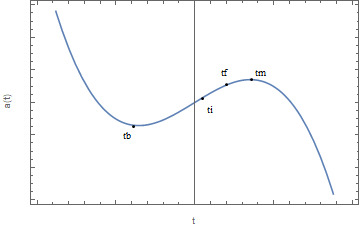
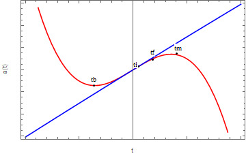
Figure 1: The scale factor of the pre-inflationary non-singular bounce evolution (left plot) and post-bounce inflationary part. In the left with red curve we present the same pre-inflationary non-singular bounce and with blue curve the pure quasi-de Sitter part of the non-singular bounce. In both cases, the matter perfect fluids are absent.

Basically, $t_{b}$ is the bouncing point which occurs before $t<0$, and $t_{m}$ would be the maximum of the scale factor after the bounce, if radiation and dark matter fluids were neglected. The physical scenario we propose is basically seen in Fig. 2. In the complete scenario, the Universe evolves from negative times, before $t_{b}$ in a contracting way, until it bounces off at the time instance $t_{b}$. After $t=0$, at the time instance $t_{i}$ the inflationary era commences which continues until $t_{f}$, in such a way that 60 $e$-foldings are accomplished. Between $t_{f}$ and $t_{i}$ the Universe is basically described by the quasi-de Sitter evolution $a(t)=a_{0}e^{H_{0}t-H_{i}^{2}t^{2}}$ and beyond that if radiation and matter fluids are ignored, the Universe’s scale factor would go to the maximum $t_{m}$ and then would decrease in a cubic exponential way. However, after inflation, the matter fluids cannot be ignored, therefore, the Universe will expand in a decelerating way following the red dashed curve.

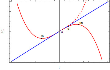
Figure 2: The scale factor of the pre-inflationary non-singular bounce evolution and post-bounce inflationary part (red curve), the pure quasi-de Sitter part of the non-singular bounce (blue curve) and the post-inflationary evolution (red dashed curve) in the presence of perfect matter fluids post-inflationary.

In this scenario, the curvature perturbations are generated during the quasi-de Sitter stage, in which the Hubble radius decreases, and the scalar quantum fluctuations are amplified thus providing the seeds for structure formation and the CMB temperature fluctuations. Before the quasi-de Sitter era, no scalar perturbations are produced, however it is interesting to note that the pre-inflationary era might affect the energy power spectrum of the primordial gravitational waves, giving an overall amplification per-inflationary amplification factor to the general relativistic waveform, as we show later on.

Interestingly enough, the scale factor (2) obeys an approximate string originating duality, namely the scale factor duality Veneziano:1991ek ; Gasperini:2007vw , which is,

$$a(t)=a^{-1}(-t)\,.$$ (3)

Indeed, when the $t^{2}$ term does not affect the evolution, the scale factor duality is satisfied by the scale factor (2), so the symmetry (3) is respected during the post-bouncing point and before the inflationary era, and after the inflationary era. It is known Gasperini:2007vw that string theories which respect this scale factor duality lead to an overall amplification of the primordial gravitational wave spectrum, and we shall examine this perspective in the context of $f(R)$ gravity.

Let us now investigate how the scale factor (2) can be realized in the context of vacuum $f(R)$ gravity. We shall be interested mainly in the quasi-de Sitter regime and the pre-inflationary regime in which the Universe evolves from the bouncing point until the beginning of the inflationary era. In the former case, the scale factor is approximately described by the quasi-de Sitter terms thus $a(t)\sim^{H_{0}t-H_{i}^{2}t^{2}}$, while in the latter case $a(t)\sim e^{-H_{b}^{3}t^{3}}$. In order to find which vacuum $f(R)$ gravity realizes these evolution patches, we shall use a well-known reconstruction technique developed in Nojiri:2009kx . To start with, we shall consider a vacuum $f(R)$ gravity theory with the following gravitational action,

$$\mathcal{S}=\frac{1}{2\kappa^{2}}\int\mathrm{d}^{4}x\sqrt{-g}f(R),$$ (4)

with $\kappa^{2}$ being as usual $\kappa^{2}=8\pi G=\frac{1}{M_{p}^{2}}$ and $M_{p}$ denotes the reduced Planck mass. The field equations are found by varying the action with respect to the metric tensor,

$$f_{R}(R)R_{\mu\nu}(g)-\frac{1}{2}f(R)g_{\mu\nu}-\nabla_{\mu}\nabla_{\nu}f_{R}(R)+g_{\mu\nu}\square f_{R}(R)=0\,,$$ (5)

where we introduced $f_{R}=\frac{\mathrm{d}f}{\mathrm{d}R}$. For the FRW metric of Eq. (1), the field equations of vacuum $f(R)$ gravity take the following form,

$$0= -\frac{f(R)}{2}+3\left(H^{2}+\dot{H}\right)f_{R}(R)-18\left(4H^{2}\dot{H}+H\ddot{H}\right)f_{RR}(R)\,,$$ (6)

$$0= \frac{f(R)}{2}-\left(\dot{H}+3H^{2}\right)f_{R}(R)+6\left(8H^{2}\dot{H}+4{\dot{H}}^{2}+6H\ddot{H}+\dddot{H}\right)f_{RR}(R)+36\left(4H\dot{H}+\ddot{H}\right)^{2}f_{RRR}\,,$$ (7)

where $f_{RR}=\frac{\mathrm{d}^{2}f}{\mathrm{d}R^{2}}$, and $f_{RRR}=\frac{\mathrm{d}^{3}f}{\mathrm{d}R^{3}}$. Now we can apply the reconstruction technique developed in Nojiri:2009kx , which is basically based on using the $e$-foldings number as a dynamical variable,

$$e^{-N}=\frac{a_{0}}{a}\,,$$ (8)

where $a_{0}$ in our case is the scale factor of the Universe at the bouncing point time instance $t_{b}$. Rewriting the Friedmann equation (6) in terms of $N$ we get,

$$-18\left[4H^{3}(N)H^{\prime}(N)+H^{2}(N)(H^{\prime})^{2}+H^{3}(N)H^{\prime\prime}(N)\right]f_{RR}+3\left[H^{2}(N)+H(N)H^{\prime}(N)\right]f_{R}-\frac{f(R)}{2}=0,$$ (9)

where the prime in the equation above, denotes differentiation with respect to $N$. Upon introducing the function $G(N)=H^{2}(N)$, the Ricci scalar takes the form,

$$R=3G^{\prime}(N)+12G(N)\,,$$ (10)

and from the above equation, by inverting it, we may obtain $N(R)$. In the case of the pure quasi-de Sitter evolution $a\sim e^{H_{0}t-H_{i}^{2}t^{2}}$, we have,

$$G(N)=H_{0}^{2}-4H_{i}^{2}N\,.$$ (11)

By combining Eqs. (10) and (11), the $e$-foldings number $N$ as a function of the Ricci scalar reads,

$$N=\frac{12H_{0}^{2}-12H_{i}^{2}-R}{48H_{i}^{2}}\,.$$ (12)

Eventually, we can rewrite the Friedmann equation as a function $G(N)$ as follows,

$$-9G(N(R))\left[4G^{\prime}(N(R))+G^{\prime\prime}(N(R))\right]F^{\prime\prime}(R)+\left[3G(N)+\frac{3}{2}G^{\prime}(N(R))\right]F^{\prime}(R)-\frac{F(R)}{2}=0,$$ (13)

with $G^{\prime}(N)=\mathrm{d}G(N)/\mathrm{d}N$ and $G^{\prime\prime}(N)=\mathrm{d}^{2}G(N)/\mathrm{d}N^{2}$. By using Eq. (12), the Friedmann equation takes the following form,

$$\left(12H_{i}^{2}\left(12H_{i}^{2}+R\right)\right)\frac{\mathrm{d}^{2}f(R)}{\mathrm{d}R^{2}}+\left(\frac{R}{4}-3H_{i}^{2}\right)R\frac{\mathrm{d}f(R)}{\mathrm{d}R}-\frac{f(R)}{2}=0,$$ (14)

which can be solved analytically and it yields the following $f(R)$ gravity solution,

$$f(R)=R+\frac{R^{2}}{72H_{i}^{2}}+2H_{i}^{2}-\frac{\mathcal{C}_{2}\left(144H_{i}^{4}+72H_{i}^{2}R+R^{2}\right)\left(\sqrt[4]{e}\sqrt{3\pi}\text{erf}\left(\frac{\sqrt{4H_{i}^{2}+\frac{R}{3}}}{4H_{i}}\right)+\frac{12H_{i}e^{-\frac{R}{48H_{i}^{2}}}\left(36H_{i}^{2}+R\right)\sqrt{12H_{i}^{2}+R}}{144H_{i}^{4}+72H_{i}^{2}R+R^{2}}\right)}{3981312H_{i}^{9}}\,,$$ (15)

where $\mathcal{C}_{2}$ is an integration constant with mass dimensions $[\mathcal{C}_{2}]=[M]^{7}$. The model (15) is a deformed $R^{2}$ model, and its phenomenology is proven to be similar to the $R^{2}$ model (this will be shown elsewhere). Specifically, for $N\sim 60$ it yields a spectral index of primordial scalar curvature perturbations $n_{s}\sim 0.967078$, irrespective of the values of the free parameters, which is very close to the value of the $R^{2}$ model, $n_{s}=0.966667$. Accordingly, the same applies for the tensor-to-scalar ratio and the tensor spectral index, which are approximately $r=0.00327846$ and $n_{T}\simeq-0.000135483$ irrespective of the values of the free parameters. The phenomenology of the model (15) is fully analyzed in another work by us, and it proves that the model is a slight deformation of the standard $R^{2}$ model. Now let us discuss which $f(R)$ gravity can realize the pre-inflationary evolution, and specifically its dominant part, namely $a(t)\sim e^{-H_{b}t^{3}}$. In this case we have,

$$G(N)\simeq 9H_{b}^{2}N^{4/3}\,,$$ (16)

at leading order in the $e$-foldings number. Again, by combining Eqs. (10) and (11), the $e$-foldings number $N$ as a function of the Ricci scalar reads,

$$N=\frac{R^{3/4}}{18\sqrt{2}\sqrt[4]{3}H_{b}^{3/2}}\,.$$ (17)

By using Eq. (12), the Friedmann equation in this case, takes the following form,

$$\left(-6\sqrt{2}\sqrt[4]{3}H_{b}^{11/2}R^{5/4}\right)\frac{\mathrm{d}^{2}f(R)}{\mathrm{d}R^{2}}+\frac{R}{4}\frac{\mathrm{d}f(R)}{\mathrm{d}R}-\frac{f(R)}{2}=0,$$ (18)

which can be solved analytically and it yields the following $f(R)$ gravity solution,

$$f(R)=\mathcal{C}_{3}\,{}_{1}F_{1}\left(-\frac{8}{3};-\frac{1}{3};\frac{R^{3/4}}{18\sqrt{2}\sqrt[4]{3}H_{b}^{11/2}}\right)-\mathcal{C}_{4}\frac{R\,_{1}F_{1}\left(-\frac{4}{3};\frac{7}{3};\frac{R^{3/4}}{18\sqrt{2}\sqrt[4]{3}H_{b}^{11/2}}\right)}{108H_{b}^{22/3}}\,,$$ (19)

where $\,{}_{1}F_{1}(a;b;z)$ is the Kummer confluent hypergeometric function, and $\mathcal{C}_{3}$, $\mathcal{C}_{4}$ are integration constants.

Having the $f(R)$ model which realizes the pre-inflationary part of the bounce, until the bouncing point, we shall now demonstrate that for the specific model, the energy spectrum of the primordial gravitational waves is overall amplified. The analysis of primordial gravitational waves in the context of $f(R)$ gravity was performed in detail in Odintsov:2021kup , so let us discuss in brief the essential features of the formalism here. For a perturbed FRW metric, the Fourier transformation of the tensor perturbation satisfies the following evolution equation,

$$\frac{1}{a^{3}f_{R}}\frac{{\rm}d}{{\rm d}t}\left(a^{3}f_{R}\dot{h}(k)\right)+\frac{k^{2}}{a^{2}}h(k)=0\,,$$ (20)

which can be cast in the following way,

$$\ddot{h}(k)+\left(3+\alpha_{M}\right)H\dot{h}(k)+\frac{k^{2}}{a^{2}}h(k)=0\,,$$ (21)

where the time-dependent parameter $\alpha_{M}$ for the $f(R)$ gravity case at hand is,

$$a_{M}=\frac{f_{RR}\dot{R}}{f_{R}H}\,.$$ (22)

The study of primordial gravitational waves evolution can be significantly simplified by adopting the WKB approach of Refs. Nishizawa:2017nef ; Arai:2017hxj , which we now describe in brief. We rewrite the evolution equation (21) of the tensor perturbations as follows,

$$h^{\prime\prime}(k)+\left(2+a_{M}\right)\mathcal{H}h^{\prime}(k)+k^{2}h(k)=0\,,$$ (23)

where the prime indicating this time differentiation with respect to the conformal time $\tau$, and $\mathcal{H}=\frac{a^{\prime}}{a}$. The WKB solution to the differential equation (23) has the following form,

$$h=e^{-\mathcal{D}}h_{GR}\,,$$ (24)

with $h_{GR}$ is the GR waveform solution of the differential equation (23) corresponding to $a_{M}=0$. Moreover, $\mathcal{D}$ is defined as follows,

$$\mathcal{D}=\frac{1}{2}\int^{\tau}a_{M}\mathcal{H}{\rm d}\tau_{1}=\frac{1}{2}\int_{0}^{z}\frac{a_{M}}{1+z^{\prime}}{\rm dz^{\prime}}\,.$$ (25)

The GR waveform produces the following energy spectrum of the primordial gravitational waves,

$$\Omega_{\rm gw}(f)=\frac{k^{2}}{12H_{0}^{2}}\Delta_{h}^{2}(k),$$ (26)

with $\Delta_{h}^{2}(k)$ being defined as Boyle:2005se ; Nishizawa:2017nef ; Arai:2017hxj ; Nunes:2018zot ; Liu:2015psa ; Zhao:2013bba ; Odintsov:2021kup ,

$$\Delta_{h}^{2}(k)=\Delta_{h}^{({\rm p})}(k)^{2}\left(\frac{\Omega_{m}}{\Omega_{\Lambda}}\right)^{2}\left(\frac{g_{*}(T_{\rm in})}{g_{*0}}\right)\left(\frac{g_{*s0}}{g_{*s}(T_{\rm in})}\right)^{4/3}\left(\overline{\frac{3j_{1}(k\tau_{0})}{k\tau_{0}}}\right)^{2}T_{1}^{2}\left(x_{\rm eq}\right)T_{2}^{2}\left(x_{R}\right),$$

and note that the “bar” in the Bessel function term, denotes the average taken over many periods. The details on the above parameters can be found in Boyle:2005se ; Nishizawa:2017nef ; Arai:2017hxj ; Nunes:2018zot ; Liu:2015psa ; Zhao:2013bba ; Odintsov:2021kup . Moreover, the term $\Delta_{h}^{({\rm p})}(k)^{2}$ denotes the primordial tensor power spectrum generated during the inflationary era, which is Boyle:2005se ; Nishizawa:2017nef ; Arai:2017hxj ; Nunes:2018zot ; Liu:2015psa ; Zhao:2013bba ; Odintsov:2021kup ,

$$\Delta_{h}^{({\rm p})}(k)^{2}=\mathcal{A}_{T}(k_{ref})\left(\frac{k}{k_{ref}}\right)^{n_{T}}\,,$$ (27)

and note that this is evaluated at the CMB pivot scale $k_{ref}=0.002$ Mpc^-1. Moreover, $n_{T}$ is the inflationary tensor spectral index and $\mathcal{A}_{T}(k_{ref})$ denotes the primordial amplitude of the tensor perturbations, which can be written in terms of the amplitude of the scalar perturbations $\mathcal{P}_{\zeta}(k_{ref})$ as follows,

$$\mathcal{A}_{T}(k_{ref})=r\mathcal{P}_{\zeta}(k_{ref})\,,$$ (28)

where $r$ is the tensor-to-scalar ratio, hence we finally have,

$$\Delta_{h}^{({\rm p})}(k)^{2}=r\mathcal{P}_{\zeta}(k_{ref})\left(\frac{k}{k_{ref}}\right)^{n_{T}}\,.$$ (29)

Combining the above, the energy spectrum for $f(R)$ gravity is,

$$\Omega_{\rm gw}(f)=e^{-2\mathcal{D}}\times\frac{k^{2}}{12H_{0}^{2}}r\mathcal{P}_{\zeta}(k_{ref})\left(\frac{k}{k_{ref}}\right)^{n_{T}}\left(\frac{\Omega_{m}}{\Omega_{\Lambda}}\right)^{2}\left(\frac{g_{*}(T_{\rm in})}{g_{*0}}\right)\left(\frac{g_{*s0}}{g_{*s}(T_{\rm in})}\right)^{4/3}\left(\overline{\frac{3j_{1}(k\tau_{0})}{k\tau_{0}}}\right)^{2}T_{1}^{2}\left(x_{\rm eq}\right)T_{2}^{2}\left(x_{R}\right)\,,$$

and recall that $\mathcal{D}$ is defined in Eq. (25). Thus what is required in order to reveal the effect of the $f(R)$ gravity, is to calculate the parameter $\mathcal{D}$ from $z=0$ up to redshift it is required. Now we are interested in ultrahigh redshifts corresponding to pre-inflationary times. In order to quantify our study, the calculation of the parameter $\mathcal{D}$ can be divided in two redshift eras, the era from present day up to redshifts corresponding to the end of inflation, and for redshifts corresponding to the end of inflation up to the bouncing point. For the calculation of the redshift, it is useful to have the relation between the redshift and the temperature of the Universe, which is approximately Garcia-Bellido:1999qrp ,

$$T=T_{0}(1+z)\,,$$ (30)

with $T_{0}$ being the present day temperature, which is 3 Kelvin, or $T_{0}=2.58651\times 10^{-4}$eV. With this relation, one can easily find the required redshifts for the calculation of the parameter $\mathcal{D}$ and subsequently the calculation of the energy power spectrum of the primordial gravitational waves. The parameter $\mathcal{D}$ will be numerically evaluated in the aforementioned redshift eras, and it is equal to,

$$\mathcal{D}=\frac{1}{2}\left(\int_{0}^{z_{f}}\frac{a_{M_{1}}}{1+z^{\prime}}{\rm dz^{\prime}}+\int_{z_{i}}^{z_{b}}\frac{a_{M_{2}}}{1+z^{\prime}}{\rm dz^{\prime}}\right)\,.$$ (31)

where $z_{f}$ is the redshift of the Universe at the end of inflation, while $z_{i}$ and $z_{b}$ denote the redshifts at the beginning of inflation and at the bouncing point. One may think that we can calculate the effects of the era before the bouncing point, however this is not possible. This is due to the fact that for the numerical calculation of the parameter $\mathcal{D}$ from present time, one uses the relation $1+z=\frac{1}{a}$, thus the scale factor at present time is unity and as the redshift increases, the scale factor decreases (we have set the present time scale factor equal to unity in order for the comoving and physical wavelengths and relevant quantities to coincide). The scale factor decreases from present time until the bouncing point, where it reaches its minimum value, and beyond the bouncing point, the scale factor increases again. Therefore the era before the bouncing point is not reachable by the present time era using $1+z=\frac{1}{a}$, it is an inaccessible era numerically. Note that the parameters $a_{M_{1}}$ and $a_{M_{1}}$ appearing in Eq. (31) both correspond to relation (22), but for different forms of the $f(R)$ gravity. Specifically, for the era between present time and the end of inflation, the $f(R)$ gravity is assumed to be described by,

$$f(R)=R+\frac{1}{M^{2}}R^{2}-\gamma\Lambda\Big{(}\frac{R}{3m_{s}^{2}}\Big{)}^{\delta}\,,$$ (32)

with $m_{s}$ in Eq. (32) being $m_{s}^{2}=\frac{\kappa^{2}\rho_{m}^{(0)}}{3}$, and $\rho_{m}^{(0)}$ is the energy density of cold dark matter today. The model (32) is basically the post-bouncing point $f(R)$ gravity plus a power-law correction term which does not affect the inflationary era, since $0<\delta<1$, but does seriously affect the late-time era. The complete lat-time study of the model (32) was performed in Ref. Odintsov:2021kup and it was shown that a viable dark energy era can be obtained and also the calculation of the the integral $\int_{0}^{z_{f}}\frac{a_{M_{1}}}{1+z^{\prime}}{\rm dz^{\prime}}$ yields the result $-0.004$, thus the amplification for this era is $\sim e^{0.00451304}=1.00452$. For the calculation of the term $\int_{z_{i}}^{z_{b}}\frac{a_{M_{2}}}{1+z^{\prime}}{\rm dz^{\prime}}$, which corresponds to the pre-inflationary and post-bouncing point era, the $f(R)$ gravity is basically that of Eq. (19). As it proves, the values of the parameters $\mathcal{C}_{3,4}$ and $H_{b}$ do not significantly affect the results, so we shall assume that $H_{b}\sim\mathcal{O}(M_{p})$ and $\mathcal{C}_{3,4}\sim\mathcal{O}(M_{p}^{2})$. Regarding the redshifts $z_{i}$ and $z_{b}$ we shall calculate them using Eq. (30). Specifically, for the redshift $z_{i}$ which corresponds to the beginning of inflation, we shall take the corresponding temperature to be the temperature of inflation, so $T_{inf}\sim 10^{15}$GeV, hence by using Eq. (30) $z_{i}$ is $z_{i}=3.86\times 10^{27}$. Regarding the bouncing point temperature, the bouncing point basically describes the most dense state in the Universe, so string theory effects should in principle be present. The classical description should also in principle fail, hence it would be inaccessible from us in the way we described above. However, for the shake of simplicity of the argument, we shall assume that we can reach it, because it proves that the final redshift does not affect significantly the calculation of the integral, at least it does not affect the result in a major and reportable way. Hence let us assume that the temperature of the bouncing point is the Planck temperature $T_{b}\sim 10^{19}$GeV hence $z_{b}\simeq 3.86\times 10^{31}$. Now the numerical calculation of the integral is easy and it yields $\int_{z_{i}}^{z_{b}}\frac{a_{M_{2}}}{1+z^{\prime}}{\rm dz^{\prime}}=-0.0338031$. Thus the overall amplification effect of the $f(R)$ gravity is $e^{-2\mathcal{D}}\sim e^{0.03831}=1.03906$. In Fig. 3 we present the $h^{2}$-scaled gravitational wave energy spectrum for pure $f(R)$ gravity and we also plot the sensitivity curves of the most important planned future gravitational waves experiments. The $f(R)$ gravity power spectrum is significantly below the sensitivity curves of the planned future experiments. Hence, although the pre-inflationary era leads to an amplification of the overall energy power spectrum, the signal is still undetectable. Thus if in future gravitational wave experiments some signal is detected in the high frequency range, this in principle will exclude $f(R)$ gravity models and all the slow-roll scalar field models, unless some exotic reheating era phenomenon takes place. Of course, the present result is model dependent and in principle some specific $f(R)$ gravity model may eventually yield a significant amplification, however it seems that $f(R)$ gravity in the presence of a scalar field might lead to a significant amplification of the primordial gravitational wave power spectrum. In Ref. Odintsov:2021kup we presented an example of that sort, however we used a Chern-Simons, however we have reportable theoretical evidence that even a simpler $f(R,\phi)$ theory can yield an amplified gravitational wave power spectrum. We shall report on this issue soon. In conclusion, amplification in $f(R)$ gravity will occur if in addition to the higher derivative terms, a scalar field is present.

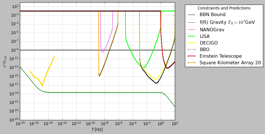
Figure 3: The $h^{2}$-scaled gravitational wave energy spectrum for pure $f(R)$ gravity.

III Conclusions

In this paper we studied an alternative evolution for our primordial Universe, which mainly consists of a non-singular bounce prior to inflation. Specifically, the Universe contracts prior to inflation until it reaches a minimum magnitude, where it bounces off and thereafter after a short period of time a quasi-de Sitter era commences. After the end of the inflationary era, the matter and radiation perfect fluids cannot be ignored, so the radiation era commences and the Universe decelerates as in ordinary post-inflationary scenarios. We investigated how these different evolution patches can be realized by vacuum $f(R)$ gravity, and we found the pre-inflationary description of the model, and in addition the inflationary quasi-de Sitter era phase, which is described by an $R^{2}$ gravity. The $R^{2}$ model in vacuum has unstable de Sitter vacua in the phase space Odintsov:2017tbc which allow a natural exit from inflation. The non-singular pre-inflationary bounce has some interesting features, for example it respects the scale factor duality during the pre-inflationary and post-inflationary era. In addition, motivated by string theory pre-inflationary scenarios which lead to an amplified gravitational wave energy spectrum, we examined whether the pre-inflationary bounce effects may lead to an amplification of the $f(R)$ gravity gravitational wave energy spectrum. As we showed in detail, indeed an overall amplification occurs for the $f(R)$ gravity theory, but the amplification is very small, and in effect, the resulting energy spectrum lies below the sensitivity curves of most future interferometer experiments. Although the result is somewhat model dependent, it seems that a pattern emerges for $f(R)$ gravity theories, in common ground with single scalar field theories, which indicates that these theories are not detectable if they are considered by themselves. Hence if a future interferometer verifies the existence of a stochastic gravitational wave background, this will indicate either that the physics are not controlled by single scalar field theory or $f(R)$ gravity, or that some exotic scenario for the reheating era takes place. Even so, one has to try hard to amplify the spectrum of $f(R)$ gravity and single scalar field theory by themselves. However, note that our conclusion about small amplification is valid only for specific pre-inflationary bounce under consideration. However, we have strong theoretical evidence which we will report soon, that a combination of higher curvature $f(R)$ gravity and non-minimally coupled scalar fields yields a considerable amplification of the gravitational wave energy spectrum, which eventually will be measurable by most, or even all the high frequency interferometer experiments. One example of this sort was reported in Odintsov:2021kup , but in the presence of exotic parity violating terms of Chern-Simons type. As we show in a future work, it is possible from a combined $f(R,\phi)$ to obtain a significant amplification for the energy spectrum of the primordial gravitational waves.

References

- (1) A. D. Linde, Lect. Notes Phys. 738 (2008) 1 [arXiv:0705.0164 [hep-th]].
- (2) D. S. Gorbunov and V. A. Rubakov, “Introduction to the theory of the early universe: Cosmological perturbations and inflationary theory,” Hackensack, USA: World Scientific (2011) 489 p;
- (3) A. Linde, arXiv:1402.0526 [hep-th];
- (4) D. H. Lyth and A. Riotto, Phys. Rept. 314 (1999) 1 [hep-ph/9807278].
- (5) K. N. Abazajian et al. [CMB-S4], [arXiv:1610.02743 [astro-ph.CO]].
- (6) M. H. Abitbol et al. [Simons Observatory], Bull. Am. Astron. Soc. 51 (2019), 147 [arXiv:1907.08284 [astro-ph.IM]].
- (7) S. Hild, M. Abernathy, F. Acernese, P. Amaro-Seoane, N. Andersson, K. Arun, F. Barone, B. Barr, M. Barsuglia and M. Beker, et al. Class. Quant. Grav. 28 (2011), 094013 doi:10.1088/0264-9381/28/9/094013 [arXiv:1012.0908 [gr-qc]].
- (8) J. Baker, J. Bellovary, P. L. Bender, E. Berti, R. Caldwell, J. Camp, J. W. Conklin, N. Cornish, C. Cutler and R. DeRosa, et al. [arXiv:1907.06482 [astro-ph.IM]].
- (9) T. L. Smith and R. Caldwell, Phys. Rev. D 100 (2019) no.10, 104055 doi:10.1103/PhysRevD.100.104055 [arXiv:1908.00546 [astro-ph.CO]].
- (10) J. Crowder and N. J. Cornish, Phys. Rev. D 72 (2005), 083005 doi:10.1103/PhysRevD.72.083005 [arXiv:gr-qc/0506015 [gr-qc]].
- (11) T. L. Smith and R. Caldwell, Phys. Rev. D 95 (2017) no.4, 044036 doi:10.1103/PhysRevD.95.044036 [arXiv:1609.05901 [gr-qc]].
- (12) N. Seto, S. Kawamura and T. Nakamura, Phys. Rev. Lett. 87 (2001), 221103 doi:10.1103/PhysRevLett.87.221103 [arXiv:astro-ph/0108011 [astro-ph]].
- (13) S. Kawamura, M. Ando, N. Seto, S. Sato, M. Musha, I. Kawano, J. Yokoyama, T. Tanaka, K. Ioka and T. Akutsu, et al. [arXiv:2006.13545 [gr-qc]].
- (14) A. Weltman, P. Bull, S. Camera, K. Kelley, H. Padmanabhan, J. Pritchard, A. Raccanelli, S. Riemer-Sørensen, L. Shao and S. Andrianomena, et al. Publ. Astron. Soc. Austral. 37 (2020), e002 doi:10.1017/pasa.2019.42 [arXiv:1810.02680 [astro-ph.CO]].
- (15) M. Kamionkowski and E. D. Kovetz, Ann. Rev. Astron. Astrophys. 54 (2016) 227 doi:10.1146/annurev-astro-081915-023433 [arXiv:1510.06042 [astro-ph.CO]].
- (16) A. Codello and R. K. Jain, Class. Quant. Grav. 33 (2016) no.22, 225006 doi:10.1088/0264-9381/33/22/225006 [arXiv:1507.06308 [gr-qc]].
- (17) S. Nojiri, S. D. Odintsov and V. K. Oikonomou, Phys. Rept. 692 (2017) 1 [arXiv:1705.11098 [gr-qc]].
-
(18)
S. Capozziello, M. De Laurentis,
Phys. Rept. 509, 167 (2011);
V. Faraoni and S. Capozziello, Fundam. Theor. Phys. 170 (2010). - (19) S. Nojiri, S.D. Odintsov, eConf C0602061, 06 (2006) [Int. J. Geom. Meth. Mod. Phys. 4, 115 (2007)].
- (20) S. Nojiri, S.D. Odintsov, Phys. Rept. 505, 59 (2011);
- (21) A. de la Cruz-Dombriz and D. Saez-Gomez, Entropy 14 (2012) 1717 [arXiv:1207.2663 [gr-qc]].
- (22) G. J. Olmo, Int. J. Mod. Phys. D 20 (2011) 413 [arXiv:1101.3864 [gr-qc]].
- (23) Y. Ema, Phys. Lett. B 770 (2017), 403-411 doi:10.1016/j.physletb.2017.04.060 [arXiv:1701.07665 [hep-ph]].
- (24) Y. Ema, K. Mukaida and J. Van De Vis, JHEP 02 (2021), 109 doi:10.1007/JHEP02(2021)109 [arXiv:2008.01096 [hep-ph]].
- (25) V. R. Ivanov and S. Y. Vernov, [arXiv:2108.10276 [gr-qc]].
- (26) S. Gottlober, J. P. Mucket and A. A. Starobinsky, Astrophys. J. 434 (1994), 417-423 doi:10.1086/174743 [arXiv:astro-ph/9309049 [astro-ph]].
- (27) A. de la Cruz-Dombriz, E. Elizalde, S. D. Odintsov and D. Sáez-Gómez, JCAP 05 (2016), 060 doi:10.1088/1475-7516/2016/05/060 [arXiv:1603.05537 [gr-qc]].
- (28) V. M. Enckell, K. Enqvist, S. Rasanen and L. P. Wahlman, JCAP 01 (2020), 041 doi:10.1088/1475-7516/2020/01/041 [arXiv:1812.08754 [astro-ph.CO]].
- (29) A. Karam, T. Pappas and K. Tamvakis, JCAP 02 (2019), 006 doi:10.1088/1475-7516/2019/02/006 [arXiv:1810.12884 [gr-qc]].
- (30) J. Kubo, J. Kuntz, M. Lindner, J. Rezacek, P. Saake and A. Trautner, JHEP 08 (2021), 016 doi:10.1007/JHEP08(2021)016 [arXiv:2012.09706 [hep-ph]].
- (31) D. Gorbunov and A. Tokareva, Phys. Lett. B 788 (2019), 37-41 doi:10.1016/j.physletb.2018.11.015 [arXiv:1807.02392 [hep-ph]].
- (32) X. Calmet and I. Kuntz, Eur. Phys. J. C 76 (2016) no.5, 289 doi:10.1140/epjc/s10052-016-4136-3 [arXiv:1605.02236 [hep-th]].
- (33) V. K. Oikonomou, Annals Phys. 432 (2021), 168576 doi:10.1016/j.aop.2021.168576 [arXiv:2108.04050 [gr-qc]].
- (34) S. Nojiri and S. D. Odintsov, Phys. Rev. D 68 (2003), 123512 doi:10.1103/PhysRevD.68.123512 [arXiv:hep-th/0307288 [hep-th]].
- (35) S. Capozziello, V. F. Cardone and A. Troisi, Phys. Rev. D 71 (2005), 043503 doi:10.1103/PhysRevD.71.043503 [arXiv:astro-ph/0501426 [astro-ph]].
- (36) J. c. Hwang and H. Noh, Phys. Lett. B 506 (2001), 13-19 doi:10.1016/S0370-2693(01)00404-X [arXiv:astro-ph/0102423 [astro-ph]].
- (37) G. Cognola, E. Elizalde, S. Nojiri, S. D. Odintsov and S. Zerbini, JCAP 02 (2005), 010 doi:10.1088/1475-7516/2005/02/010 [arXiv:hep-th/0501096 [hep-th]].
- (38) Y. S. Song, W. Hu and I. Sawicki, Phys. Rev. D 75 (2007), 044004 doi:10.1103/PhysRevD.75.044004 [arXiv:astro-ph/0610532 [astro-ph]].
- (39) T. Faulkner, M. Tegmark, E. F. Bunn and Y. Mao, Phys. Rev. D 76 (2007), 063505 doi:10.1103/PhysRevD.76.063505 [arXiv:astro-ph/0612569 [astro-ph]].
- (40) G. J. Olmo, Phys. Rev. D 75 (2007), 023511 doi:10.1103/PhysRevD.75.023511 [arXiv:gr-qc/0612047 [gr-qc]].
- (41) I. Sawicki and W. Hu, Phys. Rev. D 75 (2007), 127502 doi:10.1103/PhysRevD.75.127502 [arXiv:astro-ph/0702278 [astro-ph]].
- (42) V. Faraoni, Phys. Rev. D 75 (2007), 067302 doi:10.1103/PhysRevD.75.067302 [arXiv:gr-qc/0703044 [gr-qc]].
- (43) S. Carloni, P. K. S. Dunsby and A. Troisi, Phys. Rev. D 77 (2008), 024024 doi:10.1103/PhysRevD.77.024024 [arXiv:0707.0106 [gr-qc]].
- (44) S. Nojiri and S. D. Odintsov, Phys. Lett. B 657 (2007), 238-245 doi:10.1016/j.physletb.2007.10.027 [arXiv:0707.1941 [hep-th]].
- (45) N. Deruelle, M. Sasaki and Y. Sendouda, Prog. Theor. Phys. 119 (2008), 237-251 doi:10.1143/PTP.119.237 [arXiv:0711.1150 [gr-qc]].
- (46) S. A. Appleby and R. A. Battye, JCAP 05 (2008), 019 doi:10.1088/1475-7516/2008/05/019 [arXiv:0803.1081 [astro-ph]].
- (47) P. K. S. Dunsby, E. Elizalde, R. Goswami, S. Odintsov and D. S. Gomez, Phys. Rev. D 82 (2010), 023519 doi:10.1103/PhysRevD.82.023519 [arXiv:1005.2205 [gr-qc]].
- (48) R. H. Brandenberger, arXiv:1206.4196 [astro-ph.CO].
- (49) R. Brandenberger and P. Peter, arXiv:1603.05834 [hep-th].
- (50) D. Battefeld and P. Peter, Phys. Rept. 571 (2015) 1 doi:10.1016/j.physrep.2014.12.004 [arXiv:1406.2790 [astro-ph.CO]].
- (51) M. Novello and S. E. P. Bergliaffa, “Bouncing Cosmologies,” Phys. Rept. 463 (2008) 127 doi:10.1016/j.physrep.2008.04.006 [arXiv:0802.1634 [astro-ph]].
- (52) Y. F. Cai, Sci. China Phys. Mech. Astron. 57 (2014) 1414 doi:10.1007/s11433-014-5512-3 [arXiv:1405.1369 [hep-th]].
- (53) J. de Haro and Y. F. Cai, Gen. Rel. Grav. 47 (2015) no.8, 95 doi:10.1007/s10714-015-1936-y [arXiv:1502.03230 [gr-qc]].
- (54) S. D. Odintsov, T. Paul, I. Banerjee, R. Myrzakulov and S. SenGupta, Phys. Dark Univ. 33 (2021), 100864 doi:10.1016/j.dark.2021.100864 [arXiv:2109.00345 [gr-qc]].
- (55) I. Banerjee, T. Paul and S. SenGupta, JCAP 02 (2021), 041 doi:10.1088/1475-7516/2021/02/041 [arXiv:2011.11886 [gr-qc]].
- (56) A. A. Starobinsky, Phys. Lett. B 91 (1980), 99-102 doi:10.1016/0370-2693(80)90670-X
- (57) F. L. Bezrukov and M. Shaposhnikov, Phys. Lett. B 659 (2008), 703-706 doi:10.1016/j.physletb.2007.11.072 [arXiv:0710.3755 [hep-th]].
- (58) S. D. Odintsov and V. K. Oikonomou, Phys. Rev. D 96 (2017) no.10, 104049 doi:10.1103/PhysRevD.96.104049 [arXiv:1711.02230 [gr-qc]].
- (59) S. Nojiri, S. D. Odintsov and D. Saez-Gomez, Phys. Lett. B 681 (2009), 74-80 doi:10.1016/j.physletb.2009.09.045 [arXiv:0908.1269 [hep-th]].
- (60) G. Veneziano, Phys. Lett. B 265 (1991), 287-294 doi:10.1016/0370-2693(91)90055-U
- (61) M. Gasperini and G. Veneziano, Nuovo Cim. C 38 (2016) no.5, 160 doi:10.1393/ncc/i2015-15160-8 [arXiv:hep-th/0703055 [hep-th]].
- (62) B. E. Navascués and G. A. M. Marugán, JCAP 09 (2021), 030 doi:10.1088/1475-7516/2021/09/030 [arXiv:2104.15002 [gr-qc]].
- (63) P. R. Anderson, E. D. Carlson, T. M. Ordines and B. Hicks, Phys. Rev. D 102 (2020) no.6, 063528 doi:10.1103/PhysRevD.102.063528 [arXiv:2005.12370 [gr-qc]].
- (64) B. F. Li, P. Singh and A. Wang, Phys. Rev. D 100 (2019) no.6, 063513 doi:10.1103/PhysRevD.100.063513 [arXiv:1906.01001 [gr-qc]].
- (65) Y. Cai, Y. T. Wang and Y. S. Piao, Phys. Rev. D 92 (2015) no.2, 023518 doi:10.1103/PhysRevD.92.023518 [arXiv:1501.01730 [astro-ph.CO]].
- (66) Y. T. Wang and Y. S. Piao, Phys. Lett. B 741 (2015), 55-60 doi:10.1016/j.physletb.2014.12.011 [arXiv:1409.7153 [gr-qc]].
- (67) N. Kitazawa and A. Sagnotti, JCAP 04 (2014), 017 doi:10.1088/1475-7516/2014/04/017 [arXiv:1402.1418 [hep-th]].
- (68) M. Rinaldi, Class. Quant. Grav. 29 (2012), 085010 doi:10.1088/0264-9381/29/8/085010 [arXiv:1011.0668 [astro-ph.CO]].
- (69) S. D. Odintsov, V. K. Oikonomou and F. P. Fronimos, [arXiv:2108.11231 [gr-qc]].
- (70) A. Nishizawa, Phys. Rev. D 97 (2018) no.10, 104037 doi:10.1103/PhysRevD.97.104037 [arXiv:1710.04825 [gr-qc]].
- (71) S. Arai and A. Nishizawa, Phys. Rev. D 97 (2018) no.10, 104038 doi:10.1103/PhysRevD.97.104038 [arXiv:1711.03776 [gr-qc]].
- (72) L. A. Boyle and P. J. Steinhardt, Phys. Rev. D 77 (2008), 063504 doi:10.1103/PhysRevD.77.063504 [arXiv:astro-ph/0512014 [astro-ph]].
- (73) R. C. Nunes, M. E. S. Alves and J. C. N. de Araujo, Phys. Rev. D 99 (2019) no.8, 084022 doi:10.1103/PhysRevD.99.084022 [arXiv:1811.12760 [gr-qc]].
- (74) X. J. Liu, W. Zhao, Y. Zhang and Z. H. Zhu, Phys. Rev. D 93 (2016) no.2, 024031 doi:10.1103/PhysRevD.93.024031 [arXiv:1509.03524 [astro-ph.CO]].
- (75) W. Zhao, Y. Zhang, X. P. You and Z. H. Zhu, Phys. Rev. D 87 (2013) no.12, 124012 doi:10.1103/PhysRevD.87.124012 [arXiv:1303.6718 [astro-ph.CO]].
- (76) J. Garcia-Bellido, [arXiv:hep-ph/0004188 [hep-ph]].