On Complexity of Computing Bottleneck and Lexicographic Optimal Cycles in a Homology Class

Abstract

Homology features of spaces which appear in applications, for instance 3D meshes, are among the most important topological properties of these objects. Given a non-trivial cycle in a homology class, we consider the problem of computing a representative in that homology class which is optimal. We study two measures of optimality, namely, the lexicographic order of cycles (the lex-optimal cycle) and the bottleneck norm (a bottleneck-optimal cycle). We give a simple algorithm for computing the lex-optimal cycle for a 1-homology class in a closed orientable surface. In contrast to this, our main result is that, in the case of 3-manifolds of size $n^{2}$ in the Euclidean 3-space, the problem of finding a bottleneck optimal cycle cannot be solved more efficiently than solving a system of linear equations with an $n\times n$ sparse matrix. From this reduction, we deduce several hardness results. Most notably, we show that for 3-manifolds given as a subset of the 3-space of size $n^{2}$, persistent homology computations are at least as hard as rank computation (for sparse matrices) while ordinary homology computations can be done in $O(n^{2}\log n)$ time. This is the first such distinction between these two computations. Moreover, it follows that the same disparity exists between the height persistent homology computation and general sub-level set persistent homology computation for simplicial complexes in the 3-space.

1 Introduction

Topological features of a space are those features that remain invariant under continuous, invertible deformations of the space. Homology groups are one of the most important topological features which, while not a complete invariant of shape, nevertheless are computationally feasible and capture important structure, in the following sense. Let $\mathbb{K}$ denote our space, which we will assume is a simplicial complex. For any dimension $d$, there is a homology group $H_{d}(\mathbb{K})$ that captures the $d$-dimensional structure present. The zero dimensional group encodes the connected components of $\mathbb{K}$; the group $H_{1}(\mathbb{K})$ contains information about the closed curves in $\mathbb{K}$ which can not be “filled” in the space (often described as handles); and the group $H_{2}(\mathbb{K})$ captures the voids in the space that could not be filled, etc. For example, a hollow torus contains a single void and two classes of curves that are not “filled” in the space, and these features remain under continuous, invertible deformations of the shape.

Although the above intuitive description of the homology features is useful in many applications, in general, homology groups are algebraic objects defined for a simplicial complex (or a topological space) which do not easily translate to a canonical geometric feature. An element of a $d$-dimensional homology group is a homology class, and a homology class by definition contains a set of $d$-cycles, where cycles which are in the same class are called homologous to each other. Assume our complex $\mathbb{K}$ is a 3D mesh and $d=1$. A cycle under homology is a set of edges in the mesh, such that each vertex is incident to an even number of edges. A fixed cycle therefore corresponds to a fixed geometric feature of the mesh, while the homology class contains a large collection of these cycles. Cycles in the same class could be very different geometrically, see figure 1. Consequently, the knowledge of homology groups or Betti numbers (which are the dimensions of the homology groups) does not directly provide us with geometric features that lend themselves to interpretations that are necessary for many applications, especially in topological data analysis.

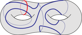
Figure 1: The blue cycle is homologous (with $\mathbb{Z}_{2}$ coefficients) to the red cycle.

Therefore, it is desirable to assign unique cycles, or those with known geometric features, to a homology class in a natural way. Much recent work has sought to define measures or weights on the cycles and then represent each homology class by some (ideally unique) cycle which optimizes that measure. This problem has been well-studied in the literature with many different measures proposed; see Section 1.2 for an overview of relevant results. Interestingly, sometimes optimizing the cycle is NP-hard and sometimes polynomial-time, depending on the measure, the classes of spaces one allows in the input, and the type of homology calculation. One of the more widely studied versions gives each edge a weight and then seeks the representative with minimum total length in the homology class. This problem is known as homology localization, and even its complexity varies widely depending on the space and the type of homology calculation. There is also a rich body of work that seeks to compute optimal cycles in persistent homology classes; again, we refer to Section 1.2 for details and citations.

In most of the paper we fix a simplicial complex $\mathbb{K}$, a fixed $d$, and a weight function given on $d$-simplices of $\mathbb{K}$. However, unlike traditional homology localization, for most of our work, it suffices to think of the weight function as an ordering of the simplices. We then consider two measures that this ordering induces on the set of $d$-cycles. The first, already defined and studied in Cohen-Steiner et al. [11], is the lexicographic ordering on the chains. The second is a minmax measure we call the bottleneck norm, which assigns to each chain the maximum weight of a simplex in it. We note that computing the lexicographic-optimal cycle is at least as hard as computing a bottleneck-optimal cycle in a given homology class, as the lexicographic-optimal cycle is always bottleneck-optimal (but the reverse is not always true). In the rest of the paper, we often shorten lexicographical-optimal to lex-optimal.

1.1 Contributions

It is proved in [11] that the persistent homology boundary matrix reduction can be used to compute the lex-optimal cycle in any given homology class in cubic time in the size of the complex, for any dimension. In this paper, we begin by presenting a new simple algorithm that, given a (closed orientable) surface and a 1-dimensional cycle, computes a lex-optimal cycle homologous to the input cycle in $O(m\log m)$ time, where $m$ is the size of a triangulation of the surface. We note that an algorithm with slightly better running-time ($O(n\alpha(n))$, where $\alpha(n)$ is the inverse Ackermann function) is also given in [11] although their algorithm only works for cycles which are homologous to a boundary and satisfy some other restrictions, see [11, Problem 17].

The simplest setting after surfaces is perhaps 3-manifolds embedded in Euclidean 3-space, for instance solid 3D meshes. For simplifying run-time comparisons, we denote the sizes of the complexes in $\mathbb{R}^{3}$ by $n^{2}$. Our main contribution in this paper is that given a system $Ax=b$ of linear equations with $A$ a sparse 0-1 matrix, it is possible to construct in $O(n^{2}\log n)$ time a 3-manifold embedded in $\mathbb{R}^{3}$ of size $O(n^{2})$ such that solving the system for a solution $x$ is equivalent to computing a bottleneck-optimal cycle in a given homology class. Our reductions remain true for integer homology and other fields $\mathbb{Z}_{p}$ (with an appropriate definition of optimal cycles), albeit with slight changes in the run-time of the reductions.

In [13], Dey presents an algorithm for computing the persistent diagram of a height function for a complex in $\mathbb{R}^{3}$ (of size $n^{2}$) in $O(n^{2}\log{n})$ time. In addition, in the same running time a set of generators can be computed. From our reduction, it follows that, if the given function on the complex (which is a mesh in $\mathbb{R}^{3}$) is not a height function, then these computations cannot be done faster than rank computation for a sparse 0-1 matrix. This gives a first answer to the main question asked in [13], asking if efficient algorithms exist for the non-height functions. In other words, our results show that there is a disparity between the efficiency of algorithms for computing sub-level-set persistence for 3D meshes of height and of general functions.

Ordinary Betti numbers for complexes in $\mathbb{R}^{3}$ (of size $n^{2}$) can be computed in $O(n^{2}\log n)$ time [12] (if a triangulation of the complement is also given). It follows from our reduction that computing persistence Betti numbers for an arbitrary function for complexes in $\mathbb{R}^{3}$ is as hard as computing the rank of a sparse 0-1 $n\times n$ matrix (even if a triangulation of the complement is given). To our knowledge, this is the first such distinction between persistent and ordinary homology computations.

We should also mention that the significance of the reductions, like the ones presented in Section 5, is not giving a lower bound for the problem in the complexity theoretic sense, as we have not done this, since we do not know if solving a sparse system has a non-trivial lower bound. Rather, the reductions show that the geometry of the problem does not help in improving trivial deterministic algorithms. For instance, one of our theorems tells a researcher of geometric methods that it is futile to try to find a deterministic $O(m\log{m})$ algorithm that computes persistent Betti numbers for meshes in 3D if that researcher is not interested in improving the best run-time for matrix rank computation for sparse matrices. As mentioned before, an $O(m\log(m))$ algorithm exists if we are interested only in height functions. Here, $m$ is size of the input mesh.

1.2 Related work

The Optimal Homologous Chain Problem (OHCP) is a well studied problem in computational topology, which specifies a particular cycle or homology class and asks for the “optimal” cycle in the same homology class. Similarly, the problem of homology localization [30] specifies a topological “feature” (usually a homology class, such as a handle or void), and asks for a representative of that class. Such representatives can be used for simplification, mesh parametrization, surface mapping, and many other problems.

Of course, computability and practicality often depend on the exact definition of “optimal”, with a wide range of variants. One natural notion of optimal is simply to assume the input complex has weights on the simplices, and to compute the representative of minimum length, area, or volume (depending on the dimension). Here, length (or area or volume) of a chain is computed as a weighted summation of the weights of its simplices; it then remains to specify the coefficients used when computing these objects, since the choice of coefficient can greatly affect the results. The resulting trade-offs can be quite subtle and surprising. For example, minimum length homologous cycles with $\mathbb{Z}$ coefficients in the homology class of highest dimension, if homology is torsion free, reduces to linear programming and hence is solvable in polynomial time [15, 7]. In contrast, with $\mathbb{Z}_{2}$ coefficients the problem is NP-hard to compute, even on 2-manifolds [6, 5]. In fact, homology localization is NP-hard to approximate for $\mathbb{Z}_{2}$ coefficients within a constant factor even when the Betti number is constant [9], and APX-Hard but fixed parameter tractable with respect to the size of the optimal cycle [2, 3]. When coefficients are over $\mathbb{Z}_{k}$, the problem becomes Unique Games Conjecture hard to approximate [22]. Homology localization has also been studied under the lens of parameterized complexity, where it is fixed parameter tractable in treewidth of the underlying complex [1].

There has been considerable followup work on different variants of homology localization. One major line of work focuses on persistent homology generators, which are often related to homology localization but seek generators in a filtration which realize a particular persistent homology class [8, 4, 25, 28, 13, 17, 16]; again, there is high variance on notions of optimality for these generators and on input assumptions, both of which affect complexity. More directly related to this paper, as noted in the introduction, lexicographic minimum cycles under some ordering on the simplices have also been studied [11].

Hardness of computing ordinary homology for complexes in Euclidean spaces is discussed in [19], where a reduction to rank computation of sparse matrices is presented; the results of this paper thus in a sense extend those of [19].

We note that there are randomized and probabilistic algorithms for sparse matrix operations in almost quadratic time [29, 10]. As a result, our reductions do not apply for these types of algorithms, since they take $O(n^{2}\log(n))$ time for a matrix with $O(n)$ non-zeros. It is natural to ask for a reduction that is linear in the size of the input $A$; indeed, this presents an interesting direction of future research.

2 Background

We begin with a brief overview of terminology and background; for more detailed coverage on these topics, we refer the reader to textbooks on topology [27] and computational topology [18, Oudot2015, DeyWang2021].

Simplicial complex

Let $V$ be a finite set. A (abstract) simplicial complex $\mathbb{K}$ is a set of subsets of $V$ such that if $\sigma\in\mathbb{K}$ and $\tau\subseteq\sigma$, then $\tau\in\mathbb{K}$. An element of $\mathbb{K}$ is called an abstract simplex. If $\sigma\in\mathbb{K}$ has $d+1$ elements then it is $d$-dimensional. The dimension of a simplicial complex is the maximum dimension of its simplices. A 0-dimensional simplex is called a vertex, a 1-dimensional simplex an edge, 2-dimensional simplex a triangle, 3-dimensional simplex a tetrahedron. The size or the complexity of a complex is the number of its simplices.

A simplex $\tau$ is called a proper face of a simplex $\sigma$ if $\tau\subset\sigma$. For a simplex $\tau\in\mathbb{K}$, the star of $\tau$ is the set of simplices $\sigma\in\mathbb{K}$ such that $\tau\subset\sigma$ and the closed star, $S(\tau)$, additionally also includes all faces of the simplices in the star. Therefore, the closed star is a simplicial complex, whereas the star is not. The link of a simplex $\tau$ is defined as $L(\tau)=\{\sigma-\tau,\sigma\in S(\tau)\}$. The link of a simplex is also a simplicial complex.

A geometric $d$-simplex is a convex hull of $d+1$ affinely independent points $\{p_{0},\ldots,p_{d}\}$ in $\mathbb{R}^{d}$. Affinely independent means that the set $\{p_{i}-p_{0},1\leq i\leq d\}$ is an independent set of vectors. We say any geometric $d$-simplex realizes an abstract $d$-simplex. Note that a face of a $d$-simplex is realized in the boundary of the geometric $d$-simplex. A simplicial complex $\mathbb{K}$ uniquely determines a topological space called its underlying space and denoted $|\mathbb{K}|$. If the complex has $n$ vertices, then all simplices of $\mathbb{K}$ are realized simultaneously in the boundary of an $(n-1)$-simplex $\Delta$. We can define $|\mathbb{K}|$ to be the union of the geometric realizations of the simplices in $\mathbb{K}$ on the boundary of $\Delta$.

The $k$-skeleton of a simplicial complex $\mathbb{K}$ is the simplicial complex which is the set of simplices of $\mathbb{K}$ of dimension at most $k$. Moreover, we note by $\mathbb{K}_{d}$ the set of $d$-simplices of $\mathbb{K}$.

A simplex-wise linear function $f:|\mathbb{K}|\rightarrow\mathbb{R}$ is a function determined by the value which it assigns to any vertex. In the relative interior of any geometric simplex the function linearly interpolates between the vertex values. Alternatively, $f$ is simplex-wise linear if the restriction of it to any geometric simplex of $|\mathbb{K}|$ is linear. We call such a function generic if the values of vertices are distinct.

We say that a simplicial complex $\mathbb{K}$ is realized in $\mathbb{R}^{3}$ or is given as a subset of $\mathbb{R}^{3}$ if there a simplex-wise linear function $f:|\mathbb{K}|\rightarrow\mathbb{R}^{3}$ which is one-to-one. Note that such a function is uniquely determined by giving the three coordinates of any vertex of $\mathbb{K}$ in $\mathbb{R}^{3}$. So, 3D meshes used in visualisation, computer graphics, etc. are simplicial complexes realized in $\mathbb{R}^{3}$.

Manifold

A (topological) $d$-manifold $M$ is a nice enough (i.e. second countable, compact, and Hausdorff) topological space with the property that every point in the space has a neighborhood that is homeomorphic to a $d$-dimensional Euclidean space or a half-space. The boundary of the manifold, $\partial M$, is the set of points of the second type.

In this paper, we work with manifolds which are underlying spaces of simplicial complexes. Such a simplicial complex is called a combinatorial manifold. For a combinatorial manifold we write $|\mathbb{K}|=M$. Intuitively, for a 2-manifold, we thus have an embedding of a the complex $\mathbb{K}$ on a some underlying surface, such that vertices are mapped to distinct points and edges are mapped to non-crossing curves. More precisely, in a 2-dimensional combinatorial manifold, $\mathbb{K}$ is mapped onto the underlying surface such that the link of a vertex is a 1-dimensional complex, i.e., a graph, and the link of an edge is a set of vertices. A simplicial complex is a combinatorial 2-manifold if and only if:

• the link of every vertex is either a simple circle or a simple path,

• the link of an edge is a pair of vertices or a single vertex.

Those vertices and edges whose links are paths and a single vertex define a subcomplex which is a combinatorial 1-manifold, whose underlying space is the boundary of the manifold $M$.

A system of loops on a 2-manifold $M$ is a set of pairwise disjoint simple loops $L$ with a common base point such that $M\setminus L$ is a topological disk. On an orientable 2-manifold, any system of loops contains exactly $2g$ loops, $g$ being the genus of $M$, and $M\setminus L$ is a $4g$-gon where each loop appears as two boundary edges; this $4g$-gon is called the polygonal schema associated with $L$. We define a cut graph of the complex $\mathbb{K}$ as a subgraph $G$ of the 1-skeleton of $\mathbb{K}$ such that $\mathbb{K}\setminus G$ is homeomorphic to a disk. Cut graphs are generalizations of the cut locus, which is essentially the geodesic medial axis of a single point. As we note above, every system of loops trivially forms a cut graph, as its removal generates a polygonal schema, but there may be many different cut graph in general.

Algorithmic approaches on combinatorial 2-manifolds are often approached via a tool called the tree-cotree decomposition [20], which is a partition of the edges of the 2-complex $\mathbb{K}$ into three sets, $T\cup Q^{*}\cup L$, where $T$ is a spanning tree of the graph, $Q^{*}$ are the dual edges of a spanning tree $Q$ of the dual graph, and $L$ is the set of leftover edges of $\mathbb{K}$. Here, a spanning tree is a tree formed by a subset of the edges in $\mathbb{K}$ such that all vertices of $\mathbb{K}$ are included. A cotree is a tree in the dual graph. The dual graph of $\mathbb{K}$ has a vertex for each triangle in $\mathbb{K}$ and two vertices are joined by an edges if the two corresponding triangles share an edge. Euler’s formula implies that $|L|=2g$. In fact, each $\ell\in L$ creates a cycle when added to $T$, and the collection of such cycles forms a system of loops, which in turn generates a polygonal schema.

A combinatorial 3-manifold $M$ is a 3-dimensional simplicial complex such that:

• the link of every vertex is a combinatorial 2-sphere or a 2-ball,

• the link of every edge is a circle or a half-circle,

• the link of every triangle is a pair of vertices or a single vertex.

Again the simplices of the second type define a combinatorial 2-manifold which is the boundary of $M$.

Homology

Consider a simplicial complex $\mathbb{K}$. A $d$-chain over the coefficient field $\mathbb{Z}_{2}$ is a formal sum of $d$-simplices: $\sum_{i}t_{i}\sigma_{i}$, where $t_{i}\in\mathbb{Z}_{2}$ and $\sigma_{i}\in\mathbb{K}_{d}$. The set of $d$-chains $C_{d}(\mathbb{K})$ is called the $d$-dimensional chain group, where we add the chains by adding coefficients. A chain can also be viewed as a set of simplices, where the simplex $\sigma_{i}$ is in the set whenever $t_{i}=1$. Under this view, addition of $d$-chains is the same as taking the symmetric difference of the simplices in each chain.

The boundary operator $\partial_{d}:C_{d}\rightarrow C_{d-1}$ is a linear transformation that to each $d$-simplex $\sigma$ assigns the set of $d-1$-simplices on its boundary. This defines $\partial_{d}$ uniquely on all the chains by linearity. A chain is called a cycle if its boundary is zero. The $d$-cycles also form a vector space which we denote by $Z_{d}(\mathbb{K})\subset C_{d}(\mathbb{K})$. A $d$-chain is called a boundary if it lies in the image of $\partial_{d+1}$. We denote the $d$-boundaries by $B_{d}(\mathbb{K})$. The most important property of the boundary operator is that for all $d\geq 0$, $\partial_{d-1}\partial_{d}=0$. This relation implies that $B_{d}(\mathbb{K})\subset Z_{d}(\mathbb{K})$. Therefore we can define the quotient

$$H_{d}(\mathbb{K})=\faktor{Z_{d}(\mathbb{K})}{B_{d}(\mathbb{K})}.$$

$H_{d}(\mathbb{K})$ is called the $d$-dimensional homology group of $\mathbb{K}$. It is also a vector space and its dimension is called the $d$-th ($\mathbb{Z}_{2}$) Betti number, denoted $\beta_{d}(\mathbb{K})$. Observe that homology classes partition the cycles. If $z\in Z_{d}(\mathbb{K})$ is a cycle we denote by $[z]\in H_{d}(\mathbb{K})$ its homology class. Two chains $c$ and $c^{\prime}$ are called homologous if $c+c^{\prime}$ is a boundary chain. Homologous cycles belong to the same homology class.

Knots and Links

A knot is a simple closed curve in $\mathbb{R}^{3}$, and a link is a set of disjoint knots in $\mathbb{R}^{3}$. Such objects are often represented and studied via link diagrams, or projections of the link to $\mathbb{R}^{2}$ which are injective except for finitely many crossings, labeled to indicate which strand is crossing over the other. See Figure 2 for a link example.

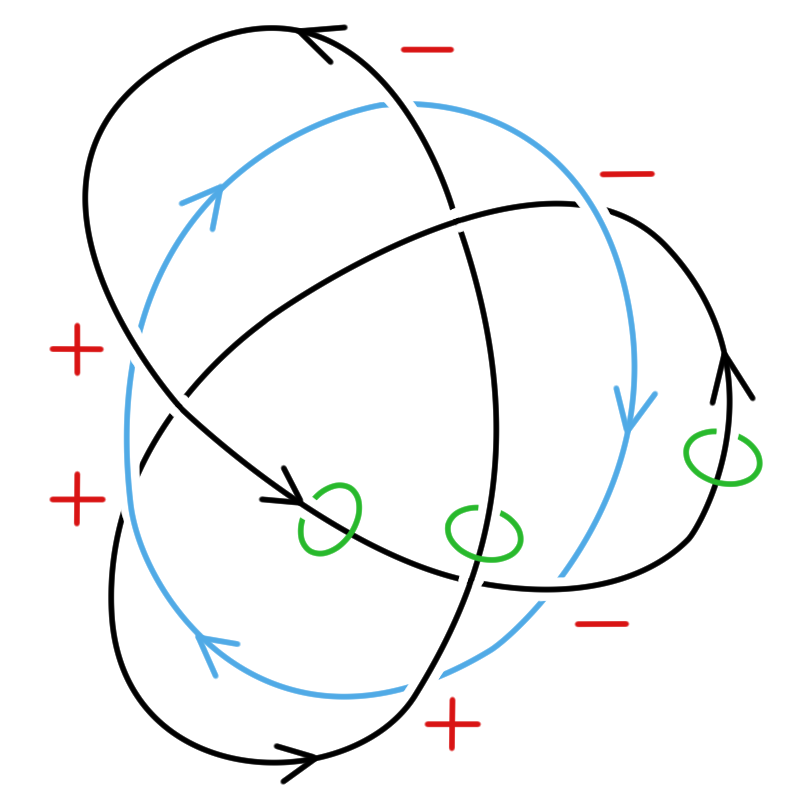
Figure 2: An example of a link diagram, with the crossing number values shown in red for each crossing; the crossing number of this knot is 0. Three meridians of the same link component of the diagram are also indicated in green.

Given a link (or knot) $L$, a tubular neighborhood is an embedding $t:L\times D^{2}\rightarrow S^{3}$ so that $t(x,0)=x$ for $x\in L$ and $D^{2}$ is an open unit disk; intuitively, this is simply a small thickening of the link that does not introduce any intersections between strands. The knot complement of $L$ is $S^{3}$ minus the tubular neighborhood. The meridian of a spatial knot is a small circle that goes around the knot. Note that regardless of where we draw meridians, they are all homologous to each other in the complement of the knot; again, see Figure 2.

The integer linking number is an invariant to quantify the linking between two closed knots, which intuitively measures the number of times that the curves wind around each other. It is not a complete invariant: Any two unlinked curves have linking number zero, but two curves with linking number zero may still be linked. These can be formalized in several different ways; see e.g. [RICCA2011], although we use a simple combinatorial characterization here: we label each crossing of the diagram as positive or negative, according to the classification shown in Figure 3. Then, the total number of positive crossings minus the total number of negative crossings is equal to twice the linking number of the diagram. This defines the integer linking number. The $\mathbb{Z}_{2}$ linking number is just the parity of the absolute value of the integer linking number, so it is either 0 or 1.

By a spatial knot or a spatial link, we mean a simple closed curve or a collection of disjoint simple closed curves respectively, in some standard 3-ball. The $\mathbb{Z}_{2}$ linking number between two spatial knots can simply be defined as follows. Take any singular disk bounded by one curve and count the intersections of the disk with the other curve. The parity of this number is the $\mathbb{Z}_{2}$ linking number.

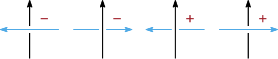
Figure 3: To compute the crossing number, each over/under crossing is labeled as shown; the crossing number is the sum of all crossing labels divided by two.

3 Bottleneck and lex-optimal cycles

Let $\mathbb{K}$ be a simplicial complex and $\mathbb{K}_{d}=\{\sigma_{0},\ldots,\sigma_{m}\}$ be the set of $d$-dimensional simplices of $\mathbb{K}$. A weight function $w$ on $\mathbb{K}_{d}$ is an arbitrary function $w:\mathbb{K}_{d}\rightarrow\mathbb{R}_{>0}=\{r\in\mathbb{R}\mid r>0\}$. Thus $w$ is defined on the generators of the chain group $C_{d}(\mathbb{K})$. For simplicity, we assume that $w$ is injective, i.e., simplices have distinct weights. For our purposes, such a weight function is equivalent to one with co-domain $\mathbb{N}-\{0\}$, or a total ordering of the simplices. If the weight function is not injective, then the edges with the same weight have exactly the same potential to appear in the optimal cycle and adding some small perturbations to their weights to distinguish them will not affect the consistency of the end result.

We extend $w$ to the function $b_{w}:C_{d}(\mathbb{K})\rightarrow\mathbb{N}$ as follows: for a chain $c\in C_{d}(\mathbb{K})$ of the form $c=\sum_{i=0}^{m}t_{i}\sigma_{i}$, where, $\forall i$, $t_{i}\in\mathbb{Z}_{2}$, we set

$$b_{w}(c)=\begin{cases}\max_{\begin{subarray}{c}0\leqslant i\leqslant m\\ t_{i}=1\end{subarray}}\{w(\sigma_{i})\}&\text{if $c\neq 0$}\\ 0&\text{if $c=0$}.\end{cases}$$

In other words, if we view a chain $c\in C_{d}(\mathbb{K})$ as a set of simplices, $b_{w}$ assigns to $c$ the maximum weight of a simplex in $c$. We call $b_{w}$ the bottleneck norm on $C_{d}(\mathbb{K})$.

By the maximum simplex, we mean the simplex with the largest weight in the chain.

Although $C_{d}(\mathbb{K})$ is a finite vector space, the function $b_{w}$ has properties analogous to a norm. First, it is non-negative. Second, assume $x$ and $y$ are chains and $\sigma_{x}$ and $\sigma_{y}$ are their maximum simplices. The maximum simplex of $x+y$ has weight at most $\max\{w(\sigma_{x}),w(\sigma_{y})\}\leq w(\sigma_{x})+w(\sigma_{y})$. Hence $b_{w}$ satisfies the triangle inequality. And third, clearly if $b_{w}(c)=0$ then $c=0$.

One can also define a lexicographic ordering on the $d$-chains based on the given weight function $w$, see also [11]. For this purpose, we order the $d$-simplices such that $\sigma<\sigma^{\prime}$ if and only if $w(\sigma)<w(\sigma^{\prime})$. We assume that the subscript of the $\sigma_{i}$ respects the order. Let $c=\sum t_{j}\sigma_{j}$ and $c^{\prime}=\sum t^{\prime}_{j}\sigma_{j}$. We define $c<_{L}c^{\prime}$ if there exists an index $j_{0}$ such that for $j>j_{0}$, $t_{j}=1$ if and only if $t^{\prime}_{j}=1$, and $t_{j_{0}}=0$, $t^{\prime}_{j_{0}}=1$. We write $c\leq_{L}c^{\prime}$ if $c<_{L}c^{\prime}$ or $c=c^{\prime}$.

3.1 Problem definitions

In this section, we give formal definitions for our two main problems, the Bottleneck-Optimal Homologous Cycle Problem (Bottleneck-OHCP) and the Lexicographic-Optimal Homologous Cycle Problem (Lex-OHCP) [11], as well as defining optimal bases for homology groups.

Bottleneck-OHCP

Given a weight function $w$ on $\mathbb{K}_{d}$, and a cycle $\zeta\in Z_{d}(\mathbb{K})$, compute a cycle $z_{*}$ such that $[z_{*}]=[\zeta]$ and such that $z_{*}$ minimizes the bottleneck norm. More formally, find $z_{*}$ such that $b_{w}(z_{*})=\min\{b_{w}(z)\mid z\in Z_{d}(\mathbb{K}),\exists c\in C_{d+1}(\mathbb{K}),z+\zeta=\partial c\}$.

In other words, the weight of the maximum simplex in $z_{*}$ is minimized in the homology class of $\zeta$. Therefore, we can also define the bottleneck weight function $b^{*}_{w}:H_{d}(\mathbb{K})\rightarrow\mathbb{R}_{\geq 0}$ on the homology classes by using the minimum $[\zeta]\mapsto b_{w}(z_{*})$. Thus the problem can also be formulated as computing the cycle which achieves $b^{*}_{w}(h)$ given any representative of the homology class $h$.

Lex-OHCP

Given a weight function $w$ on $\mathbb{K}_{d}$, and a cycle $\zeta\in Z_{d}(\mathbb{K})$, compute the cycle $z_{*}$ such that $[z_{*}]=[\zeta]$ and for any $d$-cycle $y$, if $[y]=[\zeta]$ then $z_{*}\leq_{L}y$.

We note that by our convention on the weight function, the lex-optimal cycle is always unique. Moreover, the lex-optimal cycle is also bottleneck-optimal, however, the converse is not true. Our reductions and hardness results are formulated for the bottleneck norm. Counter-intuitively, considering this intermediate problem simplifies our reductions and hardness proofs.

Optimal basis

For any suitable measure or weight function on the cycles we can define the corresponding optimal basis. Let $\leq_{p}$ be some pre-order on the set of $d$-cycles $Z_{d}(\mathbb{K})$ such that every subset $A\subset Z_{d}(\mathbb{K})$ has some chain $a$, such that $\forall z\in A,a\leq_{p}z$.

With respect to this pre-order, we define the optimal basis for $d$-homology, as a set of cycles $B\subset Z_{d}(\mathbb{K})$, representing the homology classes generating $H_{d}(\mathbb{K})$, as follows. Put the smallest non-zero element of $Z_{d}(\mathbb{K})$ in $B$. Now, repeat the following until $B$ is a representative basis for $d$-homology: let $A$ be the union of the cycles in the classes that are not in the subspace generated by the classes represented in $B$. Put the smallest cycle of $A$ in $B$.

In Section 4, we will describe a simple algorithm for computing the lex-optimal basis for the 1-dimensional homology of a surface.

3.2 The Sub-level bottleneck weight function

We defined the bottleneck weight function $b^{*}_{w}:H_{d}(\mathbb{K})\rightarrow\mathbb{N}$ on homology classes using a weight function on $d$-simplices for some fixed dimension $d$. Here we give a second, more natural definition of a generalization of this weight function. Let $\omega:|\mathbb{K}|\rightarrow\mathbb{R}$ be a generic simplex-wise linear function. The sub-level set of a value $r\in\mathbb{R}$ is the set $|\mathbb{K}|_{\leq r}=\{x\in|\mathbb{K}|\mid\omega(x)\leq r\}$. For any $d$-cycle $\zeta\in Z_{d}(\mathbb{K})$, define $b_{\omega}(\zeta):=\min\{r\in\mathbb{R}\mid\exists z\in Z^{s}_{d}(\mathbb{K}_{\leq r}),\;\exists y\in C^{s}_{d+1}(\mathbb{K}),\;\zeta+z=\partial y\},$ where $C^{s}_{\bullet}$ denotes the singular chain complex. Intuitively, $b_{\omega}(\zeta)$ is the smallest value of $r$ such that a chain homologous to $\zeta$ in $\mathbb{K}$ appears in the sub-level-set. This value of course depends only on the homology class of $\zeta$. Thus, we have a weight function $b^{*}_{\omega}:H_{d}(\mathbb{K})\rightarrow\mathbb{R}$.

Lemma 3.1.

For any weight function $w$ on $d$-simplices of $\mathbb{K}$, there is a generic simplex-wise linear function $\omega$ on the barycentric subdivision of $\mathbb{K}$, such that for any homology class $h\in H_{d}(\mathbb{K})$, $b^{*}_{\omega}(h^{\prime})=b^{*}_{w}(h)$, where $h^{\prime}$ is the image of $h$ in the subdivision.

Proof 3.2.

Let $\mathbb{K}^{\prime}$ denote the subdivision of $\mathbb{K}$. Recall that for each simplex $\sigma$ of $\mathbb{K}$ there is a vertex $v(\sigma)$ in $\mathbb{K}^{\prime}$. If $\sigma$ is a $d$-simplex, we set $\omega(v(\sigma))=w(\sigma)$. For all other vertices $v$ of $\mathbb{K}^{\prime}$ we define $b_{\omega}(v)$ to be a very small positive number. We then replace these weights with positive integers while maintaining their order. It is easy to check that our function satisfies the statement of the lemma.

Note that we use the barycentric subdivision simply to give a finer level of granularity on the sub-level sets. This subdivision appears to be necessary for the construction of the function $\omega$.

3.3 Bottleneck weight function and persistent homology

A homology class $h\in H(\mathbb{K})$ is a set of cycles such that the difference of any two of the cycles is a boundary chain. Homology classes are intuitively referred to as homological features. Persistent homology tries to measure the importance of these features. For details see [18].

Let the set of simplices of $\mathbb{K}$ be ordered such that for each simplex $\sigma$, the simplices on the boundary of $\sigma$ appear before $\sigma$ in the ordering. For instance, this ordering can be given by the time that a simplex is added, if we are building the complex $\mathbb{K}$ by adding a simplex at a time. Of course, we need the boundary of a simplex to be present before adding it. Let

$$\varnothing=\mathbb{K}_{0}\subset\mathbb{K}_{1}\cdots\subset\mathbb{K}_{n-1}\subset\mathbb{K}_{n}=\mathbb{K}$$

be the sequence of complexes such that $\mathbb{K}_{i}$ consists of the first $i$ simplices in the ordering. Such a sequence is called a filtration. For $j\geq i$, let $f^{i,j}:\mathbb{K}_{i}\subset\mathbb{K}_{j}$ be the inclusion and $f^{i,j}_{\sharp}$ the induced homomorphism on the chain groups. The homology groups $H_{d}(\mathbb{K}_{i})$ change as we add simplices. We want to track homology features during these additions.

For $0\leq i\leq j\leq n$, the $d$-dimensional persistent homology group $H^{i,j}_{d}$ is the quotient

$$H_{d}^{i,j}=\frac{f^{i,j}_{\sharp}(Z_{d}(\mathbb{K}_{i}))}{B_{d}(\mathbb{K}_{j})\cap f^{i,j}_{\sharp}(Z_{d}(\mathbb{K}_{i}))}.$$

In words, this is the group of those homology classes of $H_{d}(\mathbb{K}_{j})$ which contain cycles already existing in $\mathbb{K}_{i}$.

We give now an alternate description of the persistent homology classes. The cycles representing homology features allow us to relate the classes of different spaces to each other. We will consider, in each $\mathbb{K}_{i}$, a basis of homology and assign to each homology class in these bases a cycle which we call a p-representative cycle. Consider $\mathbb{K}_{i}$ and let $\sigma$ be a $d$-simplex such that $\mathbb{K}_{i}\cup\{\sigma\}=\mathbb{K}_{i+1}$. There are two possibilities for the change that adding $\sigma$ causes in the homology groups of $\mathbb{K}_{i}$.

1. $[\partial_{d}(\sigma)]=0$ in $\mathbb{K}_{i}$. This implies there is a $d$-chain $b$ such that $\partial_{d}(b)=\partial_{d}(\sigma)$. Therefore, $\partial_{d}(b+\sigma)=0$. It is easily seen that the cycle $z=b+\sigma$ is not a boundary in $\mathbb{K}_{i+1}$. We say that the cycle $b+\sigma$ and the class $h=[b+\sigma]$ are born at time $i+1$ or at $\mathbb{K}_{i+1}$. It follows that $H_{k}(\mathbb{K}_{i+1})=H_{k}(\mathbb{K}_{i})$ for $k\neq d$ and $H_{d}(\mathbb{K}_{i+1})=H_{d}(\mathbb{K}_{i})\oplus([z])$, where $(x)$ means the $\mathbb{Z}_{2}$-vector space generated by $x$. We take the cycle $z$ to be the p-representative for the class $h$ in $\mathbb{K}_{i+1}$. Moreover, If $z^{\prime}$ is a (inductively defined) p-representative for a homology class of $\mathbb{K}_{i}$ we transfer it to be the p-representative of its class in $\mathbb{K}_{i+1}$.

2. $[\partial_{d}(\sigma)]\neq 0$ in $\mathbb{K}_{i}$. In this case, adding the simplex $\sigma$ causes the class $h=[\partial(\sigma)]$ to become trivial. In other words, each $z\in[\partial(\sigma)]$ is now a boundary and this class is merged with the class $0$. Since the p-representatives form a basis of homology, $h$ can be written as a summation of these. The Elder Rule tells us that we declare that the youngest p-representative in this representation dies entering $\mathbb{K}_{i+1}$. Any other class still can be written as summation of existing p-representatives. Note that each p-representative now represents a possibly larger class.

For $0\leq i\leq j\leq n$, the $d$-dimensional persistent homology group $H^{i,j}_{d}$ consists of the classes, in $H_{d}(\mathbb{K}_{j})$, of those $d$-dimensional p-representatives which are born at or before $\mathbb{K}_{i}$. Therefore, the p-representatives persist through the filtration. At any $i$, they form a basis of the homology groups of $\mathbb{K}_{i}$, and their lifetime can be depicted using barcodes. The persistence diagram encodes the birth and death indices of p-representatives. Note that the non-trivial homology classes of $\mathbb{K}$ are born at some index but never die. From the above explanation the following can be observed. We omit the proof.

Proposition 3.3.

Let $h\in H_{d}(\mathbb{K}_{i})$ be a homology class and assume $h=\sum t_{j}[z_{j}]$ where $t_{j}\in\mathbb{Z}_{2}$ and the $z_{j}$ are p-representatives. Then $\sum t_{j}z_{j}$ is a bottleneck optimal cycle for $h$ (with respect to the ordering giving rise to the filtration).

Notice that there is a choice of $b$ in the first case of the case analysis above. In general, the p-representatives are not lex-optimal cycles. However, if we choose $b$ to be lex-optimal the p-representatives form a lex-optimal basis. This set of basis elements can be computed using the persistent homology boundary matrix reduction algorithm [18], as shown in [11]. This algorithm runs in $O(m^{2}\ell)$ time where $\ell$ is the number of $d$-simplices and $m$ is the number of $d+1$ simplices. Also using this basis, a lex-optimal cycle can be computed in any given class in $O(\ell^{2})$ time [11]. Of course, these algorithms also compute a bottleneck optimal cycle for any given homology class.

4 An efficient algorithm for 2-dimensional manifolds

In this section, we present a simple algorithm that, given a combinatorial 2-manifold $\mathbb{K}$, weights on the edges, and a 1-dimensional homology class, computes a lex-optimal representative cycle in the given class. For simplicity, we consider only orientable manifolds without boundary.

Our input $\mathbb{K}$ is an edge-weighted, orientable combinatorial 2-manifold, therefore, $S:=|\mathbb{K}|$ is an orientable surface without boundary. Let $m$ be the complexity of $\mathbb{K}$. Let $z$ be an input cycle on the 1-skeleton. Note that if we want an input cycle $z^{S}$ in $S$ and not in $\mathbb{K}$, i.e. the cycle is not on the 1-skeleton, then we can compute an homologous cycle $z$ on the 1-skeleton with less than $m$ edges in $O(\ell)$ time, where $\ell$ is the number of intersections of $z^{S}$ with the edges of $\mathbb{K}$.

We first construct a minimum spanning tree $T$ of the 1-skeleton of $\mathbb{K}$ with respect to the given weights. Let $G$ be the dual graph of the 1-skeleton of $\mathbb{K}$. The weight of an edge in $G$ is equal to the weight of its corresponding dual in $\mathbb{K}$. Let $Q$ be the maximum spanning co-tree of $\mathbb{K}$ in $G$ and let $Q^{*}$ be the edges of $\mathbb{K}$ whose duals are in $Q$. As shown in [20, Lemma 1] $T$ and $Q^{*}$ are disjoint. Let $L$ be the edges that are not in $T$ nor in $Q^{*}$, and recall that the triple $(T,Q,L)$ determines a polygonal schema $P$ of $4g$ sides for $S$, where $g$ is the genus of the surface. See Figure 4 as example. This means that if we cut the surface at $T\cup L$ we obtain a disk $D$, and there is an identification map $g:D\rightarrow S$ which will “re-glue” the disk into a surface. Each edge of $T\cup L$ appears twice around the disk, and each edge of $Q^{*}$ is a diagonal of this disk, connecting two vertices of the disk. The cutting of the edges of $T\cup L$ and computing the disk $D$ can be done in linear time. The two vertices of the disk that the edges in $Q^{*}$ connect can also be computed in linear time, using previous work on computing the minimal homotopic paths [14, 21].

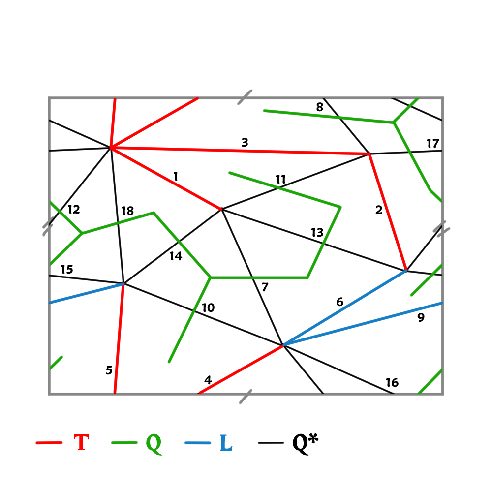
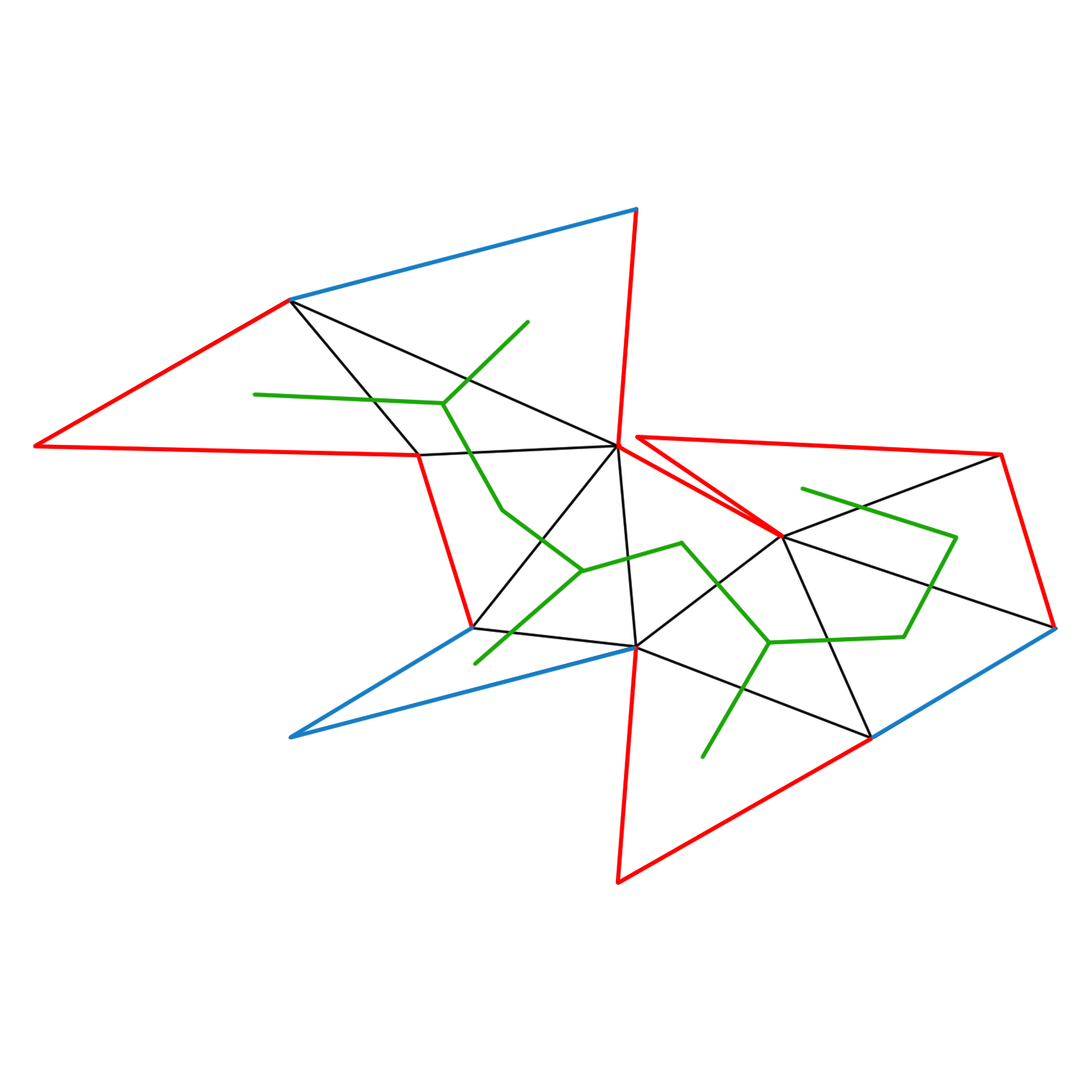
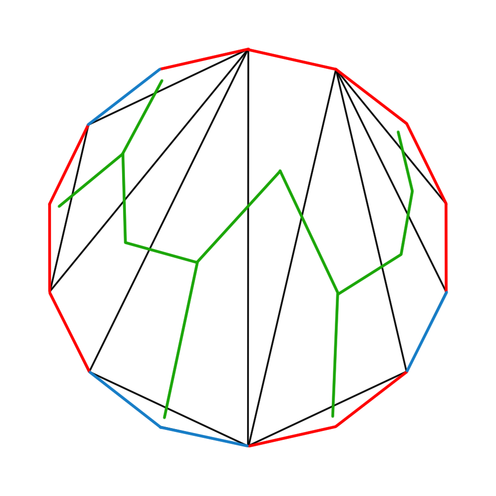
Figure 4: From left to right: a tree co-tree decomposition of a weighted, triangulated torus (with spanning tree shown in red, co-tree shown in green, and the set $L$ in blue); the same torus cut along $T\cup L$; a redrawing of the resulting polygon.

During our algorithm, we maintain a data structure $\mathcal{Z}$ which stores a circular list of elements of $\mathbb{Z}_{2}$. The circular list contains a node for each boundary edge of the disk $D$. Note that any edge of $T\cup L$ corresponds to two edges on the boundary of $D$ and thus two nodes of $\mathcal{Z}$.

Algorithm

We compute the lex-optimal cycle $z^{*}$ in the homology class of the input cycle $z$ as follows: We start with every node of $\mathcal{Z}$ at value $0$. Then, for every edge $e$ in $z$ in $T\cup L$, we set one of the two nodes corresponding to $e$ to $1$ and keep the other one at $0$. Finally, for all remaining edges $e$ in $z$, which therefore are in $Q^{*}$, let $a(e)$ be one vertex and $b(e)$ be the other vertex which $e$ connects in $D$. We add $1$ to any node whose corresponding edge of $\partial D$ is between $a(e)$ and $b(e)$ in clockwise order. At the end, we define the cycle $z^{*}$ to be the cycle consisting of edges whose two corresponding nodes in $\mathcal{Z}$ sum to $1$.

Implementation of $\mathcal{Z}$

The data structure $\mathcal{Z}$ has a single modifying operations: adding a value $1$ to any node between two given nodes (inclusive) in clockwise order. In brief, to get a constant-per-operation run-time we accumulate the operations and update the data structure in a single pass. We give now more detail. $\mathcal{Z}$ consists of an array $A$, whose cells are denoted by ‘nodes’ to avoid any confusion with complex cells. Each node represents an edge of the boundary $\partial D$ of $D$ in the right order. For any edge $e$ of $z$ in $Q^{*}$, let $a^{\prime}(e)$ be the first edge on the clockwise path between $a(e)$ and $b(e)$ in $\partial D$ and $b^{\prime}(e)$ the last edge. Additionally to a 0-1 value, each node $c$ in $A$ stores two values $s(c)$ and $f(c)$, where $s(c)$ resp. $f(c)$ is the number of edges $e$ of $z$ in $Q^{*}$ whose $a^{\prime}(e)$ resp. $b^{\prime}(e)$ corresponds to $c$. For each $e$, the cost of updating these two numbers is constant. The final cycle can be computed by first computing the value of the first node $A[0]$ and then walking along $A$ and updating the value as $A[i]=A[i-1]+s(A[i])-f(A[i-1])$.

Correctness

Let $L=\{\ell_{1},\ldots,\ell_{2g}\}$, where the $\ell_{i}$’s are sorted by increasing weight. Each edge $\ell_{i}$ defines a unique cycle when added to the tree $T$, let these cycles be denoted by $\Lambda=\{\lambda_{1},\ldots,\lambda_{2g}\}$. The following lemma is the key to our algorithm’s correctness.

lemmaqedges Let $q\in Q^{*}$. Then there is a 1-chain $c<_{L}q$ in $T\cup L$, and a 2-chain $d$ such that $\partial d=q+c$.

Proof 4.1.

The union of the edges in $T$ and $L$ form a cut graph $G$ of the surface, in the sense that the closure of $S-|G|$ is a topological disk $D$. Every edge of $T\cup L$ appears twice on the boundary of $D$, and any $q\in Q^{*}$ is a diagonal in the polygon $D$. Let $p_{1}$ and $p_{2}$ be the two arcs such that $\partial D=p_{1}\cup p_{2}$ and the endpoints of $p_{1}$ and $p_{2}$ coincide with those of $q$. Let $\tilde{p}_{i}\in C_{1}(\mathbb{K})$ be the 1-chain corresponding to $p_{i}$, $i=1,2$, i.e., $\tilde{p}_{i}=g_{\sharp}(p_{i})$. Recall that $g_{\sharp}$ is the induced map on chain groups. Let $d_{1}$ be the 2-chain bounded by $p_{1}$ and $q$ and let $\tilde{d}_{1}=g_{\sharp}(d_{1})$. We have $\partial\tilde{d}=q+\tilde{p}_{1}$, where by $q$ we denote this edge in $D$ and $S$. We now claim that every edge in $\tilde{p}_{1}$ is smaller than $q$. Note that $\tilde{p}_{1}$ is a chain of $T\cup L$. We consider two cases. First, assume $\tilde{p}_{1}$ consists only of edges of $T$. In this case, it equals the unique path in $T$ defined by the endpoints of $q$. Since $T$ is a minimum spanning tree our claim is proved.

Second, assume that $\tilde{p}_{1}$ is not entirely in $T$. In this case we argue as follows. Let $\ell\in L$ and let $\ell_{1}$ and $\ell_{2}$ be the two copies of $\ell$ on $\partial D$. We claim that if $\ell_{1}$ and $\ell_{2}$ are on both of the arcs $p_{1}$ and $p_{2}$ (that is, if $\ell_{1}\in p_{1}$ and $\ell_{2}\in p_{2}$ or $\ell_{2}\in p_{1}$ and $\ell_{1}\in p_{2}$) then $\ell<q$. Assume for the sake of contradiction that $\ell>q$. Under these conditions, if we remove the dual of $q$ from $Q$ and add the dual of $\ell$, we have reconnected the spanning co-tree split by removing $q$ (since the effect of removing $q$ from $Q$ is adding it to $L$ and thus cutting the disk $D$ at $q$ while the effect of adding $\ell$ to $Q-\{q\}$ is merging the resulting disks at $\ell_{1}$ and $\ell_{2}$, thus again forming a single disk). Thus we have increased the weight of the spanning co-tree which is not possible. Therefore, $\ell<q$ or the two copies of $\ell$ appear on one of $p_{1}$ or $p_{2}$. It follows that every edge of $L$ (which appears once) in $\tilde{p}_{1}$ is smaller than $q$ (since appearing twice cancels an edge). To finish the proof in this case, we claim that for every edge $t\in T\cap\tilde{p}_{1}$ there is an edge $\ell\in L\cap\tilde{p}_{1}$ such that $t<\ell$. It then follows that $\tilde{p}_{1}<q$.

To prove the claim we argue as follows. $T\cup L$ is a graph on the 1-skeleton of $K$ and it is standard and easy to show that any homology class $0\neq h\in H_{1}(K)$ contains exactly one cycle of $T\cup L$. Let $z=q+x$ be the cycle formed by adding $q$ to $T$, where $x$ is the path on $T$. We have $z+\partial{\tilde{d}_{1}}=z+\tilde{p}_{1}+q=\tilde{p}_{1}+x=:z^{\prime}$ and $z^{\prime}$ is a non-empty cycle in $T\cup L$ (If $z^{\prime}$ were empty then $\tilde{p}_{1}=x$, this is not possible since $x$ is in $T$ and $\tilde{p}_{1}$ is not in $T$ by assumption). Thus $z^{\prime}$ can also be written as a non-empty summation of the $\lambda_{i}$. Each $\lambda_{i}$ has the property that its unique edge $\ell_{i}\in L$ is larger than its edges in $T$. Since these $\ell_{i}$ are never cancelled, it follows that for each edge $t\in z^{\prime}\cap T$ there is an edge $\ell\in z^{\prime}\cap L$ such that $t<\ell$. Since the $L$-edges are in $\tilde{p}_{1}$ and not in $x$ our claim is proved.

With some abuse of notation we also denote the chain on $\partial D$ defined by the nodes of $\mathcal{Z}$ with value 1 by $\mathcal{Z}$. Note that in the beginning of the algorithm $g_{\sharp}({\mathcal{Z}})=z$. The algorithm then repeatedly updates $\mathcal{Z}$ by adding the chain $p_{1}$ returned by the above lemma to $\mathcal{Z}$ and adding the chain $\tilde{p}_{1}=g_{\sharp}(p_{1})$ to $z$. It updates $\mathcal{Z}$ such that at any time $g_{\sharp}({\mathcal{Z}})=z$. To finish the proof of correctness, it remains to show that the final cycle, namely the unique cycle $z_{*}$ of $T\cup L$ in the class of $z$, is indeed the lex-min cycle. To see this, assume on the contrary that there is a cycle $y$ such that $[y]=[z]$ and $y<z_{*}$. Since there is a unique cycle of any class in $T\cup L$, $y$ has to contain an edge of $Q^{*}$ hence can be made smaller, which contradicts minimality of $y$. Therefore, the cycles of $T\cup L$ are indeed the lex-min representatives of homology classes.

theoremlexoptalg Let $\mathbb{K}$ be a simplicial complex which is a closed orientable combinatorial 2-manifold and let $m$ be its number of simplices. There is an algorithm that computes a lex-optimal basis for the 1-dimensional homology of $\mathbb{K}$ in $O(m\log(m))$ time. Moreover, we can compute a lex-optimal representative for any given 1-homology class within the same run-time.

Proof 4.2.

We have proved that the algorithm correctly computes the lex-optimal cycle homologous to $z$. We show that the basis $\Lambda$ is lex-optimal basis. First note that by Lemma 4 every non-trivial cycle $y$ is homologous to a cycle $y^{\prime}\leq_{L}y$ such that $y^{\prime}$ is a subset of $T\cup L$. Since these must contain some $\ell_{i}$, it follows that the smallest non-trivial cycle contains only $\ell_{1}$ and edges of $T$, and hence is $\lambda_{1}$.

Assume inductively that $\Lambda_{i}=\{\lambda_{1},\ldots,\lambda_{i}\}$ is a lex-optimal basis for the vector space $(\Lambda_{i})\subset H_{1}(\mathbb{K})$. We claim that $\lambda_{i+1}$ is the smallest cycle in classes in the set $H_{1}-(\Lambda_{i})$. Consider any non-trivial cycle $y$ and decrease it to $y^{\prime}$ as above. To see that $\lambda_{i+1}$ is the smallest cycle, note that $y^{\prime}\cap L$ must contain some $l_{j}$ larger than $\lambda_{i}$, since otherwise $[y]\in(\Lambda_{i})$; the smallest cycle with this property is $\lambda_{i+1}$.

Constructing $T$, the dual graph and $Q$ takes at most $O(m\log m)$ time. Since we perform one update operation on $\mathcal{Z}$ per edges of $Q$ the total running time is $O(m\log m)$.

5 Reductions

In this section, we first reduce solving a system of linear equation $Ax=b$, with $A$ sparse, to computing the bottleneck-optimal homologous cycle problem for a 3-manifold given as a subset of the Euclidean 3-space. We then use this reduction to deduce hardness results for similar homological computations for 3-manifolds and 2-complexes in 3-space. Due to space constraints, some proofs of this section can only be found in the full version of the paper.

Let $A=(a_{ij})$, $i,j\in\{1,\ldots,n\}$, be an $n\times n$ square matrix with values in $\mathbb{Z}_{2}$. Let $A_{i}$ denote the $i$-th column, and $A^{t}_{i}$ denote the $i$-the row of $A$. Let $x=(x_{1},\ldots,x_{n})$ be the vector of the $n$ variables of the system $Ax=b$, and $b=(b_{1},\ldots,b_{n})$.

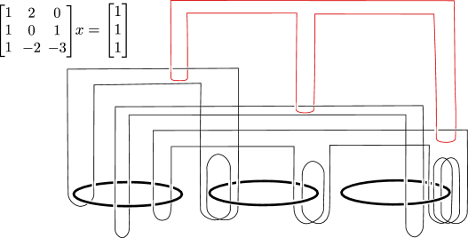
Figure 5: This figure is a link diagram for the reduction of the indicated linear system. The thick round circles are the $\lambda_{i}$, and the link components are drawn in thin black and red. For all of the crossings between ${\mathcal{L}}_{i}$, the vertical strand goes over the horizontal strand. In other words, these are not linked with each other. Note that in this example we are using integer matrix and integer linking number to showcase how the reduction works for integers. In the text we are concerned with 0-1 matrices. One also sees here how the need for generating large linking numbers (in absolute value) increases the complexity of the reduction.

From the given system $Ax=b$, we first construct a link diagram ${\mathcal{L}}^{\prime}$. We start by drawing $n$ round circles in the plane, whose collection we denote by $\Lambda^{\prime}=\{\lambda^{\prime}_{1},\ldots,\lambda^{\prime}_{n}\}$; see the thick circles in the Figure 5 for an illustration. For each row $A^{t}_{i}$ of $A$, we draw a component of the link ${\mathcal{L}}^{\prime}$, denoted $L^{\prime}_{i}$, such that its linking number is non-zero with $\lambda^{\prime}_{j}$ if and only if $a_{ij}=1$; this can be accomplished simply by linking $L_{i}^{\prime}$ appropriately with $\lambda^{\prime}_{i}$ depending on the value of $a_{ij}$. As we wish the $L_{i}$’s to not link with each other, any crossings between a fixed $L_{i}$ and $L_{j}$ are simply set to be all over (or all under), so that they will remain unlinked. Again, we refer to Figure 5, where example knots $L^{\prime}_{1},L_{2}^{\prime}$, and $L_{3}^{\prime}$ are depicted by thin black lines. We add one final knot, which we denote as $\zeta^{\prime}$, to the link ${\mathcal{L}}^{\prime}$ so that its linking number with $\lambda_{i}^{\prime}$ is non-zero if and only if $b_{i}=1$; this can be accomplished by linking $\zeta^{\prime}$ once with each $L_{i}^{\prime}$. See the top knot shown in red in Figure 5 for an illustration.

lemmalinkcrossings Let $A$ be such that each row of $A$ has at most $c$ non-zero entries. Then the link diagram ${\mathcal{L}}^{\prime}$ has $O(cn^{2})$ crossings.

In the next step, we construct a spatial link ${\mathcal{L}}$ from the link diagram ${\mathcal{L}}^{\prime}$, such that the knots appear in the 1-skeleton of a triangulation of a 3-ball. This is standard and can be done in $O(m\log(m))$-time where $m$ is the number of crossings of the link diagram ${\mathcal{L}}^{\prime}$ [23, Lemma 7.1]. The resulted space has complexity $O(m)$. Our diagram has $O(n^{2})$ many crossings, therefore this construction takes $O(n^{2}\log{n})$ time and we obtain triangulation of a ball with complexity $O(n^{2})$. The spatial link ${\mathcal{L}}$ corresponding to ${\mathcal{L}}^{\prime}$ is a set of disjoint simple closed curves in the 1-skeleton of a triangulation of a 3-ball $B^{3}$. We denote the spatial knots corresponding to $L^{\prime}_{i}$ by $L_{i}$, and analogously we name other components of ${\mathcal{L}}$.

Consider the sub-link $\mathcal{N}$ of ${\mathcal{L}}$ consisting of the components $L_{i}$. We define the manifold $M$ to be the link-complement of the link $\mathcal{N}$. This link-complement, by definition, is obtained by removing the interior of a thin polyhedral tubular neighborhood of each component of $\mathcal{N}$. This construction is again standard, and a triangulation of $M$ can be constructed in linear time form the spatial link [23]. Therefore, the 3-manifold $M$ is a subset of a 3-ball $B^{3}$, and has $n$ boundary components. By extra subdivisions, if necessary, we can make sure that in the interior of $M$, $\zeta$, $\lambda_{i}$ and $b$ are simple, disjoint, closed curves in the 1-skeleton. To do this, it is enough to make sure this property holds in every tetrahedron.

The cycle $\zeta$ is the input cycle in our instance of the bottleneck-optimal homologous cycle problem. We still need to define our edge weights, which will be based on an ordering of the edges of $M$. Let $\{e_{ij}\}$ be the set of edges in the cycle $\lambda_{i}$. First, we make sure that every edge not in some $\lambda_{i}$ is larger than any $e_{ij}$. Second, if $i<i^{\prime}$, we make sure that, for all $j,j^{\prime}$, $e_{ij}$ is smaller than $e_{i^{\prime}j^{\prime}}$. This finishes construction of our problem instance.

Let $\mu_{i}$, $i\in\{1,\ldots,n\}$, be meridians of the knots $L_{i}$ in $M$. This is a circle on the boundary component of $M$ corresponding to $L_{i}$. It is well-known that the homology group $H_{1}(M)$ is a $\mathbb{Z}_{2}$-vector space with the basis $\{[\mu_{1}],\ldots,[\mu_{n}]\}$ isomorphic to $\mathbb{Z}_{2}^{n}$.

lemmareduction The following hold:

1. If there is a vector $x\in\mathbb{Z}_{2}^{n}$ such that $Ax=b$ then any bottleneck-optimal cycle in the class $[\zeta]$ is a summation of the cycles $\lambda_{j}$.

2. If there exists a bottleneck-optimal cycle $z_{*}$ in the class $[\zeta]$ such that $z_{*}=\sum_{i=1}^{n}x_{i}\lambda_{i}$ then the vector $x=(x_{1},\ldots,x_{n})^{t}$ is a solution to $Ax=b$.

Proof 5.1.

First, observe that for the class $[\lambda_{j}]$ we have $[\lambda_{i}]=\sum_{j=1}^{n}a_{ji}[\mu_{j}]$. The left of Figure 6 depicts a 2-chain realizing this relation. If we map the basis element $[\mu_{j}]$ to the $j$-th standard basis element $e_{j}$, then we have defined an isomorphism $H_{1}(M)\cong\mathbb{Z}_{2}^{n}$ in which the class $[\lambda_{i}]$ maps to the column $A_{i}$. Second, note that, with a similar argument, $[\zeta]=\sum_{i=1}^{n}b_{j}[\mu_{j}]$, see Figure 6 right. Thus $[\zeta]$ maps to $b$ under the isomorphism. It follows that $Ax=b$ if and only if $\sum x_{j}[\lambda_{j}]=[\zeta]$. The second statement follows.

If $x$ is a solution to $Ax=b$, then the cycle $z=\sum x_{j}\lambda_{j}$ belongs to the class $[\zeta]$. Any cycle which is not entirely a subset of the edges of the $\lambda_{i}$’s, and hence a summation of the $\lambda_{i}$, contains some edge which is larger than all the edges of the $\lambda_{i}$’s and therefore has weight more than $z$. It follows that any bottleneck-optimal cycle is a summation of the $\lambda_{i}$ or, a subset of them, since these are disjoint simple cycles. This proves the first statement.

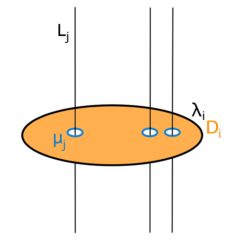
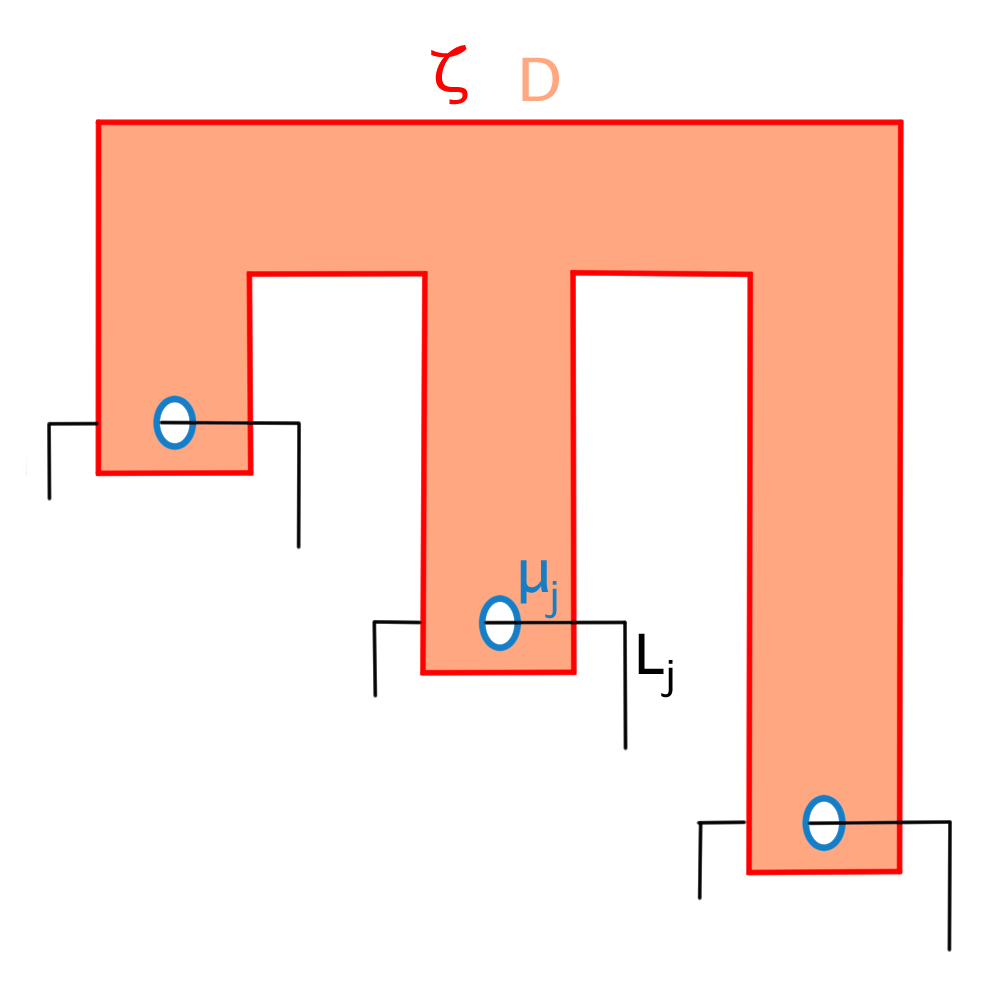
Figure 6: $\partial D_{i}=\lambda_{i}+\sum_{j}a_{ji}\mu_{j}$ (left), $\partial D=\zeta+\sum_{j}b_{j}\mu_{j}$ (right).

theoremsparsematrix Solving the system of equations $Ax=b$ where $A$ is a sparse $\mathbb{Z}_{2}$-matrix reduces in $O(n^{2}\log n)$ time to the bottleneck-optimal homologous cycle problem with $\mathbb{Z}_{2}$-coefficients for a 3-manifold of size $O(n^{2})$ given as a subset of $\mathbb{R}^{3}$.

Proof 5.2.

Given the system $Ax=b$ we have already constructed our instance. If the bottleneck-optimal cycle $z_{*}$ returned by any algorithm that solves the Bottleneck-OHCP problem uses only edges in $\bigcup\lambda_{i}$, then the second statement of Lemma 5 implies that we can find a solution by determining which $\lambda_{i}$ appear in $z_{*}$. This can be done in linear time. On the other hand, if $z_{*}$ uses some edge not in $\bigcup\lambda_{i}$, then there is no solution to the system by the first statement of Lemma 5.

Although we have not defined the integer homology groups, it is almost immediate that the above reduction works also with $\mathbb{Z}$-coefficients.

Corollary 5.3.

The (1-dimensional) lex-optimal homologous cycle problem for 3-manifolds in $\mathbb{R}^{3}$ of size $n^{2}$ cannot be solved more efficiently than the time required to solve a system of equations $Ax=b$ with $A$ a sparse $n\times n$ matrix, if the latter time is $\Omega(n^{2}\log(n))$.

As noted before, the persistent boundary reduction algorithm can compute a lex-optimal cycle in $O(lm^{2})$ time [11], where $m$ is the number of $d+1$-simplices and $l$ is the number of $d$-simplices. Although a set of persistent generators can be computed in matrix multiplication time [26], we do not know that the lex-optimal cycle can be found in matrix multiplication time, as it is unclear if the divide and conquer strategy from [26] would work on our problem.

corollarymmtime A set of sub-level-set persistent homology generators for a 3-manifold $M$ or a 2-complex $\mathbb{K}$ of size $n^{2}$ in $\mathbb{R}^{3}$ and a generic simplex-wise linear function $f:M\rightarrow\mathbb{R}$ cannot be computed more efficiently than the time required to compute a maximal set of independent columns in an $n\times n$ sparse matrix $A$, if the latter time is $\Omega(n^{2}\log(n))$.

Proof 5.4.

Recall that in our reduction above, the cycles $\lambda_{i}$ correspond to columns of the matrix $A$. After a subdivision, we can define a simplex-wise linear function such that bottleneck weight function equals the sub-level set bottleneck weight function, by Lemma 3.1. With respect to this function, the (subdivision of the) cycles $\lambda_{i}$ are the first cycles in their homology classes that appear in a sub-level set. Only an independent set of these cycles will remain until the end. These cycles therefore determine a subset of the columns of $A$ which are independent.

For the 2-complex $\mathbb{K}$, we can simply take the 2-skeleton of the manifold in the reduction. There will be no change in 1-dimensional persistent homology groups.

As noted in the introduction, the above results are in a strong contrast with the results of Dey [13]. In other words, if the complex is of size $O(n^{2})$ and the given function on the simplicial complex $\mathbb{K}$ is a height function then one can compute the generators in $O(n^{2}\log n)$ time, whereas, for a general function, one cannot do better than computing a maximal set of independent columns for a given sparse matrix $A$ of size $n$. To the best of our knowledge, the best deterministic algorithm for this operation takes at least $O(n^{\omega})$ time, where $\omega$ is the exponent of matrix multiplication.

corollarythreemanifold The persistence diagram for a 2-complex or a 3-manifold of size $n^{2}$ in $\mathbb{R}^{3}$ and a generic simplex-wise linear function $f:|\mathbb{K}|\rightarrow\mathbb{R}$ cannot be computed more efficiently than the time required to compute the rank of a sparse $n\times n$ matrix $A$, if the latter time is $\Omega(n^{2}\log(n))$.

Proof 5.5.

The number of 1-dimensional points with infinite death times and which correspond to the $\lambda_{i}$ is the number of independent columns of $A$. We can determine if a point belongs to a $\lambda_{i}$ by checking its birth time. The point represents some $\lambda_{i}$ if and only if the birth time is smaller than the weight of edges not contained in these cycles.

Again the above theorem should be compared with results of [13], where the persistence is computed in $O(n^{2}\log n)$ time for a 2-complex in 3-space of size $n^{2}$ and a height function.

References

- [1] Nello Blaser and Erlend Raa Vågset. Homology localization through the looking-glass of parameterized complexity theory, 2020. \hrefhttp://arxiv.org/abs/2011.14490 \patharXiv:2011.14490.
- [2] Glencora Borradaile, William Maxwell, and Amir Nayyeri. Minimum bounded chains and minimum homologous chains in embedded simplicial complexes. In Proceedings of the 36th International Symposium on Computational Geometry (SoCG 2020). Schloss Dagstuhl-Leibniz-Zentrum für Informatik, 2020.
- [3] Oleksiy Busaryev, Sergio Cabello, Chao Chen, Tamal K. Dey, and Yusu Wang. Annotating simplices with a homology basis and its applications. In Fedor V. Fomin and Petteri Kaski, editors, Algorithm Theory – SWAT 2012, pages 189–200, 2012.
- [4] Oleksiy Busaryev, Tamal K. Dey, and Yusu Wang. Tracking a generator by persistence. In My T. Thai and Sartaj Sahni, editors, Computing and Combinatorics, pages 278–287, 2010.
- [5] Erin W. Chambers, Jeff Erickson, Kyle Fox, and Amir Nayyeri. Minimum cuts in surface graphs, 2019. \hrefhttp://arxiv.org/abs/1910.04278 \patharXiv:1910.04278.
- [6] Erin W. Chambers, Jeff Erickson, and Amir Nayyeri. Minimum cuts and shortest homologous cycles. In Proceedings of the 25th International Symposium on Computational Geometry (SoCG 2009). ACM Press, 2009. \hrefhttps://doi.org/10.1145/1542362.1542426 \pathdoi:10.1145/1542362.1542426.
- [7] Erin W. Chambers and Mikael Vejdemo-Johansson. Computing minimum area homologies. Computer Graphics Forum, 34(6):13–21, November 2014. \hrefhttps://doi.org/10.1111/cgf.12514 \pathdoi:10.1111/cgf.12514.
- [8] Chao Chen and Daniel Freedman. Measuring and computing natural generators for homology groups. Computational Geometry, 43(2):169–181, 2010. Special Issue on the 24th European Workshop on Computational Geometry (EuroCG’08). \hrefhttps://doi.org/10.1016/j.comgeo.2009.06.004 \pathdoi:10.1016/j.comgeo.2009.06.004.
- [9] Chao Chen and Daniel Freedman. Hardness results for homology localization. Discrete & Computational Geometry, 45(3):425–448, January 2011. \hrefhttps://doi.org/10.1007/s00454-010-9322-8 \pathdoi:10.1007/s00454-010-9322-8.
- [10] Ho Yee Cheung, Tsz Chiu Kwok, and Lap Chi Lau. Fast matrix rank algorithms and applications. Journal of the ACM, 60(5), October 2013. \hrefhttps://doi.org/10.1145/2528404 \pathdoi:10.1145/2528404.
- [11] David Cohen-Steiner, André Lieutier, and Julien Vuillamy. Lexicographic Optimal Homologous Chains and Applications to Point Cloud Triangulations. In 36th International Symposium on Computational Geometry (SoCG 2020), pages 32:1–32:17. Schloss Dagstuhl–Leibniz-Zentrum für Informatik, 2020. \hrefhttps://doi.org/10.4230/LIPIcs.SoCG.2020.32 \pathdoi:10.4230/LIPIcs.SoCG.2020.32.
- [12] Cecil Jose A. Delfinado and Herbert Edelsbrunner. An incremental algorithm for Betti numbers of simplicial complexes on the 3-sphere. Computer Aided Geometric Design, 12(7):771–784, 1995. \hrefhttps://doi.org/10.1016/0167-8396(95)00016-Y \pathdoi:10.1016/0167-8396(95)00016-Y.
- [13] Tamal K. Dey. Computing height persistence and homology generators in efficiently. In Proceedings of the 30th Annual ACM-SIAM Symposium on Discrete Algorithms (SODA 2019), page 2649–2662, USA, 2019. Society for Industrial and Applied Mathematics.
- [14] Tamal K. Dey and Sumanta Guha. Transforming curves on surfaces. Journal of Computer and System Sciences, 58(2):297–325, 1999. \hrefhttps://doi.org/doi.org/10.1006/jcss.1998.1619 \pathdoi:doi.org/10.1006/jcss.1998.1619.
- [15] Tamal K. Dey, Anil N. Hirani, and Bala Krishnamoorthy. Optimal homologous cycles, total unimodularity, and linear programming. SIAM Journal on Computing, 40(4):1026–1044, January 2011. \hrefhttps://doi.org/10.1137/100800245 \pathdoi:10.1137/100800245.
- [16] Tamal K. Dey, Tao Hou, and Sayan Mandal. Persistent 1-cycles: Definition, computation, and its application, 2018. \hrefhttp://arxiv.org/abs/1810.04807 \patharXiv:1810.04807.
- [17] Tamal K. Dey, Tao Hou, and Sayan Mandal. Computing minimal persistent cycles: Polynomial and hard cases. In Proceedings of the 31st Annual ACM-SIAM Symposium on Discrete Algorithms (SODA 2020), page 2587–2606, USA, 2020. Society for Industrial and Applied Mathematics.
- [18] Herbert Edelsbrunner and John Harer. Computational Topology: an Introduction. American Mathematical Society, 2010.
- [19] Herbert Edelsbrunner and Salman Parsa. On the computational complexity of betti numbers: Reductions from matrix rank. In Proceedings of the 25th Annual ACM-SIAM Symposium on Discrete Algorithms (SODA 2014), pages 152–160. Society for Industrial and Applied Mathematics, 2014. \hrefhttps://doi.org/10.1137/1.9781611973402.11 \pathdoi:10.1137/1.9781611973402.11.
- [20] David Eppstein. Dynamic generators of topologically embedded graphs. In Proceedings of the 14th Annual ACM-SIAM Symposium on Discrete Algorithms (SODA 2003), pages 599–608. Society for Industrial and Applied Mathematics, 2003.
- [21] Jeff Erickson and Kim Whittlesey. Transforming curves on surfaces redux. In Proceedings of the 24th Annual ACM-SIAM Symposium on Discrete Algorithms (SODA 2013). Society for Industrial and Applied Mathematics, January 2013. \hrefhttps://doi.org/10.1137/1.9781611973105.118 \pathdoi:10.1137/1.9781611973105.118.
- [22] Joshua A. Grochow and Jamie Tucker-Foltz. Computational topology and the unique games conjecture. In Proceedings of 34th International Symposium on Computational Geometry (SoCG 2018). Schloss Dagstuhl-Leibniz-Zentrum fuer Informatik, 2018.
- [23] Joel Hass, Jeffrey C. Lagarias, and Nicholas Pippenger. The computational complexity of knot and link problems. Journal of the ACM (JACM), 46(2):185–211, 1999.
- [24] A. Hatcher. Algebraic Topology. Cambridge University Press, 2002. URL: \urlhttps://pi.math.cornell.edu/ hatcher/AT/AT.pdf.
- [25] Yasuaki Hiraoka, Takenobu Nakamura, Akihiko Hirata, Emerson G. Escolar, Kaname Matsue, and Yasumasa Nishiura. Hierarchical structures of amorphous solids characterized by persistent homology. Proceedings of the National Academy of Sciences, 113(26):7035–7040, June 2016. \hrefhttps://doi.org/10.1073/pnas.1520877113 \pathdoi:10.1073/pnas.1520877113.
- [26] Nikola Milosavljević, Dmitriy Morozov, and Primoz Skraba. Zigzag persistent homology in matrix multiplication time. In Proceedings of the 27th International Symposium on Computational Geometry (SoCG 2011), page 216–225, New York, NY, USA, 2011. ACM. \hrefhttps://doi.org/10.1145/1998196.1998229 \pathdoi:10.1145/1998196.1998229.
- [27] James R. Munkres. Elements of algebraic topology. CRC press, 2018.
- [28] Ippei Obayashi. Volume-optimal cycle: Tightest representative cycle of a generator in persistent homology. SIAM Journal on Applied Algebra and Geometry, 2(4):508–534, January 2018. \hrefhttps://doi.org/10.1137/17m1159439 \pathdoi:10.1137/17m1159439.
- [29] Douglas H. Wiedemann. Solving sparse linear equations over finite fields. IEEE Transactions on Information Theory, 32(1):54–62, 1986. \hrefhttps://doi.org/10.1109/TIT.1986.1057137 \pathdoi:10.1109/TIT.1986.1057137.
- [30] Afra Zomorodian and Gunnar Carlsson. Localized homology. Computational Geometry, 41(3):126–148, November 2008. \hrefhttps://doi.org/10.1016/j.comgeo.2008.02.003 \pathdoi:10.1016/j.comgeo.2008.02.003.