Alpaqa: A matrix-free solver for nonlinear MPC and large-scale nonconvex optimization

Abstract

This paper presents alpaqa, an open-source C++ implementation of an augmented Lagrangian method for nonconvex constrained numerical optimization, using the first- order panoc algorithm as inner solver. The implementation is packaged as an easy-to-use library that can be used in C++ and Python. Furthermore, two improvements to the panoc algorithm are proposed and their effectiveness is demonstrated in NMPC applications and on the cutest benchmarks for numerical optimization. The source code of the alpaqa library is available at https://github.com/kul-optec/alpaqa and binary packages can be installed from https://pypi.org/project/alpaqa.

I Introduction

I-A Background and motivation

Large-scale optimization problems arise naturally in many areas of science and engineering. As the models used in these different application domains are becoming increasingly complex, the need arises for solvers that can handle large, nonconvex optimization problems. For instance, in the field of systems and control, the demand for improved autonomy in dynamical, complex and uncertain environments have boosted the importance of optimal control under nonlinear dynamics and long prediction horizons. This in turn yields nonconvex and large-scale optimization problems.

One of the core motivations for the present work is the requirement for real-time solution of nonconvex optimization problems in the context of nonlinear model predictive control (NMPC). The real-time requirement, and often limited hardware capabilities available on embedded devices, result in a need for efficient solvers, both in terms of computation and memory.

Classical techniques for solving NMPC problems include sequential quadratic programming (SQP) and interior point (IP) methods. An advantage of SQP is that the solver can be warm-started using (a shifted version of) the solution of the previous time step, and techniques like real-time iteration (RTI) require the solution of just a single QP at each time step. Interior point methods are popular general-purpose solvers, and state-of-the-art implementations such as Ipopt [1] are fast and easy to use. A disadvantage of interior point methods for model predictive control is that they cannot easily be warm-started, although some techniques do exist [2].

Another family of algorithms for constrained optimization that saw increased interest in the past decade are Augmented Lagrangian methods (ALM) [3]. These methods involve the successive minimization of the augmented Lagrangian function, an exact penalty function for the original constrained optimization problem. The minimization problems in the inner loop of the ALM algorithm have simpler constraints than the original problem (often box constraints), and can be solved using a wide range of existing solvers. Thanks to the use of a penalty function, ALM can cope with large numbers of constraints. Moreover, by repeatedly solving similar problems, ALM naturally takes advantage of warm-starting the inner solver. These properties render it particularly suitable for MPC applications, where a good initial guess is typically available.

In this work, ALM is used to tackle general nonconvex constraints, and the recently developed method called panoc (Proximal Averaged Newton-type method for Optimal Control) [4] is used as an inner solver. Panoc is a quasi-Newton-accelerated first-order method, which – despite its simple, inexpensive iterations – enjoys locally superlinear convergence, without requiring the manipulation of large Jacobian or Hessian matrices. Applying ALM and penalty-based methods combined with panoc has recently proven successful within several applications in NMPC [5, 6] and the Optimization Engine (OpEn) software [7], which shares some of its algorithmic foundations with the present work, although it is tailored more heavily towards embedded systems applications.

I-B Contributions

The main contribution of this paper is alpaqa (Augmented Lagrangian Proximal Averaged Quasi-Newton Algorithms), an open-source software package that provides efficient C++ implementations of an augmented Lagrangian method and different variants of panoc. The solvers can be used both directly from C++ and from Python through a user-friendly interface based on CasADi [8].

Furthermore, we propose two modifications to panoc that significantly improve the practical performance and robustness of the algorithm: Section III exploits the structure of the derivatives of the objective function when applied to box-constrained problems, and Section IV introduces an alternative line search condition to help reject poor quasi-Newton steps that harm the practical convergence. In Section V, the effectiveness of these modifications is demonstrated by applying the alpaqa implementation to an NMPC problem and a subset of the cutest benchmark collection.

Notation

Let $[a,b]$ denote the closed interval from $a$ to $b$. $\N_{[i,j]}\triangleq[i,j]\cap\N$ is the inclusive range of natural numbers from $i$ to $j$. The set of extended real values is denoted as $\overline{\Re}\triangleq\Re\cup\{+\infty\}$. Uppercase calligraphic letters are used for index sets. $x_{i}$ refers to the $i$’th component of $x\in\Re^{n}$. Given an index set $\mathcal{I}=\{i_{1},\,\dots,\,i_{m}\}\subseteq\N_{[1,n]}$, we use the shorthand $x_{\mathcal{I}}=(x_{i_{1}},\,\dots,\,x_{i_{m}})$. For $u,v\in\Re^{n}$, let $u\leq v$ denote the component-wise comparison. Given a positive definite matrix $\Sigma$, define the $\Sigma$-norm as $\|x\|_{\Sigma}\triangleq\sqrt{x^{\!\top}\Sigma\,x}$, and the distance in $\Sigma$-norm of a point $x$ to a set $C$ as $\operatorname{dist}_{\Sigma}(x,C)\triangleq\min\left\{\|x-v\|_{\Sigma}\;\mid\;v\in C\right\}$. The proximal operator of function $h:\Re^{n}\rightarrow\overline{\Re}$ is defined as $\operatorname{prox}_{\gamma h}(x)\triangleq\min_{w}\big{\{}h(w)+\tfrac{1}{2\gamma}\left\|w-x\right\|^{2}\big{\}}$, and the Moreau envelope of $h$ is defined as the value function of $\operatorname{prox}_{\gamma h}$, $h^{\gamma}(x)\triangleq\inf_{w}\big{\{}h(w)+\tfrac{1}{2\gamma}\left\|w-x\right\|^{2}\big{\}}$ [9, Def. 1.22].

II Problem statement and preliminaries

We propose a numerical optimization solver for general nonconvex nonlinear programs of the form

$$\underset{x}{\text{minimize}} f(x)$$ (P)

subject to $$\underline{x}\leq x\leq\overline{x}$$

$$\underline{z}\leq g(x)\leq\overline{z},$$

with the objective function $f:\Re^{n}\rightarrow\Re$ and the constraints function $g:\Re^{n}\rightarrow\Re^{m}$ possibly nonconvex.

Define the rectangular sets $C$ and $D$ as the cartesian products of one-dimensional closed intervals, $C_{i}\triangleq[\underline{x}_{i},\overline{x}_{i}],\;C\triangleq C_{1}\times\dots\times C_{n}$ and $D_{i}\triangleq[\underline{z}_{i},\overline{z}_{i}],\;D\triangleq D_{1}\times\dots\times D_{m}$, such that the constraints of Problem (P) can be written as $x\in C$ and $g(x)\in D$.

For completeness, we briefly review the augmented Lagrangian method and the panoc algorithm [3, 4], including a minor modification to the ALM penalty factor, following [10]. The methods described in this section serve as the algorithmic foundation for alpaqa. In Sections III and IV, we subsequently describe included improvements to these basic methods.

II-A Augmented Lagrangian method

The general constraints $g(x)\in D$ in Problem (P) are relaxed by introducing a slack variable $z$ and by applying an augmented Lagrangian method to the following problem:

$$\underset{x\in C,\;z\in D}{\text{minimize}} f(x)$$ (P-ALM)

subject to $$z=g(x).$$

Given a diagonal, positive definite $m$-by-$m$ matrix $\Sigma$, define the augmented Lagrangian function $\operatorname{\mathcal{L}}_{\Sigma}:\Re^{n}\times\Re^{m}\times\Re^{m}\rightarrow\Re$ with penalty factor $\Sigma$ as

$$\operatorname{\mathcal{L}}_{\Sigma}(x,z,y)\,\triangleq\,\operatorname{\mathcal{L}}(x,z,y)+\tfrac{1}{2}\left\|g(x)-z\right\|^{2}_{\Sigma},$$ (1)

where $\operatorname{\mathcal{L}}(x,z,y)=f(x)+\langle y,g(x)-z\rangle$ denotes the standard Lagrangian.

The augmented Lagrangian method for solving Problem (P-ALM) then consists of repeatedly (1) minimizing $\operatorname{\mathcal{L}}_{\Sigma}$ with respect to the decision variables $x$ and the slack variables $z$ (2) updating the Lagrange multipliers $y$ (3) increasing the penalty factors $\Sigma_{ii}$ corresponding to constraints with high violation. This procedure is shown in Algorithm 1. The minimization problem in step (1) is solved up to a tolerance $\varepsilon^{\nu}$ with $\lim_{\nu\rightarrow\infty}\varepsilon^{\nu}=0$ such that $\left\|x^{\nu}-\Pi_{C}\big{(}x^{\nu}-\nabla_{\!x}\!\operatorname{\mathcal{L}}_{\Sigma}(x^{\nu},z^{\nu},y^{\nu})\big{)}\right\|_{\infty}\leq\varepsilon^{\nu}$, with $x^{\nu}\in C,\,z^{\nu}\in D$. The solution $(x^{\nu},\,y^{\nu})$ is returned when the termination criteria $\left\|g(x^{\nu})-z^{\nu}\right\|_{\infty}\leq\delta$ and $\varepsilon^{\nu}\leq\varepsilon$ are satisfied, for given tolerances $\varepsilon$ and $\delta$.

Algorithm 1 Augmented Lagrangian Method

procedure ALM($x^{0}$, $y^{0}$, $\Sigma^{0}$)

    for $\nu=1,2,\dots$ do

        $(x^{\nu},z^{\nu})\leftarrow\underset{x\in C,\;z\in D}{\text{{argmin}}}\quad\operatorname{\mathcal{L}}_{\Sigma^{\nu-1}}(x,\,z;\,y^{\nu-1})$ $\triangleright$ (1)

        $y^{\nu}\leftarrow\Pi_{Y}\left(y^{\nu-1}+\Sigma^{\nu-1}\left(g(x^{\nu})-z^{\nu}\right)\right)$ $\triangleright$ (2)

        $\Sigma^{\nu}\leftarrow$ Update_$\Sigma$$(x^{\nu},\,z^{\nu},\,x^{\nu-1},\,z^{\nu-1},\,\Sigma^{\nu-1}$)$\triangleright$ (3)     

function Update_$\Sigma$($x^{\nu}$, $z^{\nu}$, $x^{\nu-1}$, $z^{\nu-1}$, $\Sigma^{\nu-1}$)

    $e^{\nu}\leftarrow g(x^{\nu})-z^{\nu}$

    $e^{\nu-1}\leftarrow g(x^{\nu-1})-z^{\nu-1}$

    $\Sigma^{\nu}\leftarrow\Sigma^{\nu-1}$

    for $i=1,2,\dots,m$ do

        if $|e^{\nu}_{i}|>\theta|e^{\nu-1}_{i}|$ then

           $\Sigma^{\nu}_{ii}\leftarrow\Sigma^{\nu-1}_{ii}\,\max\left\{1,\;\Delta\dfrac{|e^{\nu}_{i}|}{\|e^{\nu}\|_{\infty}}\right\}$             

    return $\Sigma^{\nu}$

The use of a diagonal matrix $\Sigma$ as penalty factor – with a separate penalty factor for each constraint, rather than a single scalar for all constraints – was inspired by the qpalm solver [10]. Qpalm uses the same heuristic to update the penalty factors, where the increase in the penalty for a given constraint depends on the violation of that constraint relative to the total constraint violation.

II-B Panoc

The inner minimization problem in step (1) of Algorithm 1 will be solved by the panoc algorithm [4]. Panoc solves problems of the form:

$$\underset{x}{\text{minimize}} \psi(x)+h(x),$$ (P-PANOC)

where $\psi:\Re^{n}\rightarrow\Re$ is real-valued and $h:\Re^{n}\rightarrow\overline{\Re}$ allows efficient computation of the proximal operator. Recall that in (1), our aim is to solve

$$\min_{x\in C,\,z\in D}\operatorname{\mathcal{L}}_{\Sigma}(x,z,y) =\min_{x\in C}\big{\{}\psi_{\Sigma}(x;y)\big{\}}-\tfrac{1}{2}\lVert y\rVert_{\Sigma^{-1}}^{2},$$ (2)

where

$$\psi_{\Sigma}(x;y) \triangleq f(x)+\min_{z\in D}\left\{\tfrac{1}{2}\left\|z-\left(g(x)+\Sigma^{-1}y\right)\right\|_{\Sigma}^{2}\right\}$$ (3)

$$=f(x)+\tfrac{1}{2}\text{dist}_{\Sigma}^{2}\left(g(x)+\Sigma^{-1}y,\ D\right).$$

The minimizer $z^{\nu}=\Pi_{D}\left(g(x^{\nu})+\Sigma^{-1}y\right)$ can be computed directly. Setting $\psi(x)=\psi_{\Sigma}(x;y)$ and $h=\delta_{C}$, the indicator function of $C$, it is clear that panoc is indeed applicable to the problem at hand.

The main idea behind panoc is to select the next iterate as a convex combination of a proximal gradient step and a quasi-Newton step: Iteration using proximal gradient steps is slow, but convergence to a stationary point can be guaranteed, whereas the quasi-Newton steps are faster, but only convergent close to a local minimum. A line search is used as a globalization strategy, preserving the global convergence of the proximal gradient algorithm, while preferring quasi-Newton steps whenever possible to speed up the algorithm. A popular quasi-Newton method is limited-memory BFGS (L–BFGS) [11, Algorithm 2].

To set the stage for the proposed improvements in the following sections, we now introduce the necessary details regarding panoc. Let the forward-backward operator $T_{\gamma}:\Re^{n}\rightrightarrows\Re^{n}$ denote the set of proximal gradient steps in $x$, i.e.,

$$T_{\gamma}(x) \triangleq\operatorname{prox}_{\gamma h}\big{(}x-\gamma\nabla\psi(x)\big{)}$$ (4)

$$=\operatorname*{\arg\!\min}_{w}\left\{h(w)+\tfrac{1}{2\gamma}\left\|x-\gamma\nabla\psi(x)-w\right\|^{2}\right\}.$$

Local solutions of (P-PANOC) are fixed points of $T_{\gamma}$, and roots of the fixed-point residual $R_{\gamma}(x)\triangleq\frac{1}{\gamma}\left(x-T_{\gamma}(x)\right)$. Let $H_{k}$ be an operator that is in some sense close to the inverse Jacobian of the fixed-point residual $R_{\gamma}(x)$. Then for a given step size $\gamma$, the next panoc iterate is computed as

$$\hat{x}^{k} \in T_{\gamma}(x^{k})$$ (5a)

$$p^{k} =\hat{x}^{k}-x^{k}$$ (5b)

$$q^{k} =-H_{k}R_{\gamma}(x^{k})=-\gamma^{-1}H_{k}p^{k}$$ (5c)

$$x^{k+1} =x^{k}+(1-\tau)\,p^{k}+\tau\,q^{k}.$$ (5d)

The parameter $\tau\in[0,1]$ is selected using a backtracking line search over the forward-backward envelope (FBE) [13], an exact, continuous, real-valued penalty function for the inner problem (P-PANOC). More specifically, let the parameter $\sigma\in\left(0,\;\tfrac{1-\gamma L}{2\gamma}\right),$ where the step size $\gamma$ and the parameter $L\in\left(0,\gamma^{-1}\right)$ are chosen such that the following quadratic upper bound is satisfied:

$$\psi(\hat{x}^{k})\leq\psi(x^{k})+\nabla\psi(x^{k})^{\top}(\hat{x}^{k}-x^{k})+\tfrac{L}{2}\lVert\hat{x}^{k}-x^{k}\rVert^{2}.$$ (6)

Then, panoc uses the sufficient decrease condition

$$\varphi_{\gamma}(x^{k+1})\leq\varphi_{\gamma}(x^{k})-\sigma\lVert p^{k}\rVert^{2},$$ (7)

where $\varphi_{\gamma}:\Re^{n}\rightarrow\Re$ is the FBE defined as

$$\varphi_{\gamma}(x) \triangleq\psi(x)-\tfrac{\gamma}{2}\|\nabla\psi(x)\|^{2}+h^{\gamma}(x-\gamma\nabla\psi(x)),$$ (8)

and $p^{k}$ is the proximal gradient step as defined in (5b).

When these conditions hold, it can be shown that when $\tau=0$ or $x^{k+1}=\hat{x}^{k}$, the line search condition (7) is satisfied, and global convergence of the algorithm can be demonstrated by telescoping equation (7) [4, Thm. III.3].

At each iterate, condition (6) is satisfied using the procedure outlined in Algorithm 2. If the gradient of $\psi$ is $L_{\psi}$-Lipschitz continuous, then the while loop will terminate, because condition (6) holds whenever $L\geq L_{\psi}$. If $\nabla\psi$ is only locally Lipschitz and if the domain is bounded, then the maximum value of $L$ can be bounded as well, again implying the termination of Algorithm 2. [4, Remark III.4] The original panoc algorithm is listed in Algorithm 3.

Algorithm 2 Step size selection

function update_step_size($x$, $\gamma$, $L$)

    $\hat{x}\leftarrow T_{\gamma}(x)$,    $p\leftarrow\hat{x}-x$

    while  $\psi(\hat{x})>\psi(x)+\nabla\psi(x)^{\top}p+\tfrac{L}{2}\lVert p\rVert^{2}$  do

        $\gamma\leftarrow\gamma/2$,    $L\leftarrow 2L$

        $\hat{x}\leftarrow T_{\gamma}(x)$,    $p\leftarrow\hat{x}-x$     

    return $\gamma$, $L$

Algorithm 3 panoc

1:procedure panoc($x^{0}$, $\gamma_{0}$, $L_{0}$)

2:    for $k\leftarrow 0,1,2,\dots$ do

3:        $p^{k}\leftarrow T_{\gamma_{k}}(x^{k})-x^{k}$ $\triangleright$ Proximal gradient step

4:        $q^{k}\leftarrow-\gamma^{-1}H_{k}p^{k}$ $\triangleright$ Quasi-Newton step

5:        $\tau\leftarrow 1$

6:        do$\triangleright$ Line search

7:           $x^{k+1}\leftarrow x^{k}+(1-\tau)\,p^{k}+\tau\,q^{k}$

8:           $\tau\leftarrow\tau/2$

9:        while $\varphi_{\boldsymbol{\gamma_{k}}}(x^{k+1})>\varphi_{\gamma_{k}}(x^{k})-\sigma_{k}\lVert p^{k}\rVert^{2}$

10:        $\gamma_{k+1}$, $L_{k+1}$ $\leftarrow$ update_step_size($x^{k+1}$, $\gamma_{k}$, $L_{k}$)     

III Structured panoc

In the original panoc algorithm, $h$ was essentially allowed to be any proximable mapping. Since for our purposes, $h$ in (P-PANOC) is taken to be the indicator of $C$, its proximal operator reduces to a projection onto the box, i.e., $\operatorname{prox}_{\gamma\delta_{C}}(x)=\operatorname*{\arg\!\min}_{w\in C}\big{\{}\tfrac{1}{2\gamma}\left\|w-x\right\|^{2}\big{\}}=\Pi_{C}(x)$. This results in an inexpensive component-wise operation and furthermore induces some additional structure, which we may exploit to replace line 4 in Algorithm 3, which was originally implemented using a general L–BFGS strategy. This results in a more efficient variant of panoc, which is better tailored to our particular purpose.

To this end let us first define the set of indices corresponding to active box constraints on $x$ after a gradient step,

$$\mathcal{K}(x) \triangleq\left\{\;i\in\N_{[1,n]}\;\left|\;\begin{aligned} &x_{i}-\gamma\nabla_{x_{i}}\psi(x)\leq\underline{x}_{i}\\ \;\;\vee\;\;&\overline{x}_{i}\leq x_{i}-\gamma\nabla_{x_{i}}\psi(x)\end{aligned}\right.\right\}$$ (9)

and its complement $\mathcal{J}(x)\triangleq\N_{[1,n]}\setminus\mathcal{K}(x)$ (inactive constraint indices). For ease of notation, let $P_{\mathcal{K}\mathcal{J}}$ denote a row permutation matrix that reorders all rows with indices $k\in\mathcal{K}(x)$ before the rows with indices $j\in\mathcal{J}(x)$.

A straightforward calculation reveals that if $\nabla\psi$ and the fixed-point residual $R_{\gamma}=\gamma^{-1}(I-T_{\gamma})$ are differentiable at $x$, the Jacobian $\jac R_{\gamma}(x)$ is given by

$$\jac R_{\gamma}(x)=P_{\mathcal{K}\mathcal{J}}^{\top}\begin{pmatrix}\gamma^{-1}I&0\\ \nabla^{2}_{\!x_{\mathcal{J}}x_{\mathcal{K}}}\!\psi(x)&\nabla^{2}_{\!x_{\mathcal{J}}x_{\mathcal{J}}}\!\psi(x)\end{pmatrix}P_{\mathcal{K}\mathcal{J}},$$ (10)

using which we may apply a semismooth Newton method to the problem of finding roots of $R_{\gamma}$, replacing the quasi-Newton step $q^{k}=-H_{k}R_{\gamma}(x^{k})$. The Newton step $q$ is computed as the solution to the system of equations

$$\begin{pmatrix}\gamma^{-1}I&0\\ \nabla^{2}_{\!x_{\mathcal{J}}x_{\mathcal{K}}}\!\psi(x)&\nabla^{2}_{\!x_{\mathcal{J}}x_{\mathcal{J}}}\!\psi(x)\end{pmatrix}\;P_{\mathcal{K}\mathcal{J}}\,q=-P_{\mathcal{K}\mathcal{J}}\,R_{\gamma}(x).$$ (11)

Defining $\begin{pmatrix}q_{\mathcal{K}}\\ q_{\mathcal{J}}\end{pmatrix}\triangleq P_{\mathcal{K}\mathcal{J}}\,q$, this can be written as

$$q_{\mathcal{K}} =x_{\mathcal{K}}-T_{\gamma}(x)_{\mathcal{K}}$$ (12a)

$$\nabla^{2}_{\!x_{\mathcal{J}}x_{\mathcal{J}}}\!\psi(x)\,q_{\mathcal{J}} =-\nabla_{\!x_{\mathcal{J}}}\psi(x)-\nabla^{2}_{\!x_{\mathcal{J}}x_{\mathcal{K}}}\!\psi(x)\,q_{\mathcal{K}}.$$ (12b)

Here, the Hessian of $\psi$ is given by

$$\nabla^{2}\psi(x)= \nabla^{2}f(x)+\sum_{i\in\mathcal{A}(x)}\nabla^{2}g_{i}(x)\,\hat{y}_{i}(x)$$ (13)

$$\phantom{\nabla^{2}f(x)}+\sum_{i\in\mathcal{A}(x)}\Sigma_{ii}\,\nabla g_{i}(x)\nabla g_{i}(x)^{\top}$$

where

$$\mathcal{A}(x)=\left\{\;i\in\N_{[1,m]}\;\left|\;\begin{aligned} &g_{i}(x)+\Sigma_{ii}^{-1}y_{i}<\underline{z}_{i}\\ \;\;\vee\;\;&\overline{z}_{i}<g_{i}(x)+\Sigma_{ii}^{-1}y_{i}\end{aligned}\right.\right\}$$ (14)

is the set of indices of the active (nonlinear) constraints, and
$\hat{y}(x)\triangleq\Sigma\,\left(g(x)+\Sigma^{-1}y-\Pi_{D}\left(g(x)+\Sigma^{-1}y\right)\right).$

Equation (12a) can be computed without any additional work, because these components of the Newton step are equal to the projected gradient step, $q_{\mathcal{K}}=p_{\mathcal{K}}$.
Equation (12b) on the other hand requires the solution of a (smaller) linear system using part of the Hessian of the augmented Lagrangian function, $\nabla^{2}_{\!x_{\mathcal{J}}x_{\mathcal{J}}}\!\psi$.

Sections III-A and III-B present different strategies for solving the system (12b).

III-A Direct solution using the Hessian of the augmented Lagrangian

A first approach to compute the step $q_{\mathcal{J}}$ in equation (12b) is to solve it directly using standard techniques such as $LDL^{\top}$ or Cholesky factorization. If the block $\nabla^{2}_{\!x_{\mathcal{J}}x_{\mathcal{J}}}\!\psi(x)$ of the Hessian is not positive definite, a modified Cholesky factorization [14], or a conjugate gradients method [15, §7] can be used.

A disadvantage of this approach is that, in general, the Hessian of the augmented Lagrangian $\nabla^{2}\psi$ could be dense, even if the Hessian of the Lagrangian $\nabla^{2}_{\!xx}\!\operatorname{\mathcal{L}}$ is sparse, because of the rightmost term in equation (13). For large-scale optimization problems, computing, storing and factorizing this dense Hessian is often prohibitively expensive.

III-B Solution using the Hessian of the Lagrangian and the Jacobian of the constraints

Using the equation (13), the Hessian of the augmented Lagrangian can be written in terms of the Hessian of the Lagrangian and the Jacobian of the constraints, with the goal of exploiting the sparsity of these matrices.

For ease of notation, define the matrices
$H_{\!\mathcal{J}}\triangleq\Big{.}\nabla_{\!x_{\mathcal{J}}x_{\mathcal{J}}}^{2}\!\operatorname{\mathcal{L}}(x,y)\Big{|}_{\big{(}x,\,\hat{y}(x)\big{)}}\;\text{and}\;\;G_{\!\mathcal{J}}\triangleq\nabla_{\!{x_{\!\mathcal{J}}}}g_{\mathcal{A}}(x).$
Then (12b) is equivalent to the following linear system

$$\begin{pmatrix}H_{\!\mathcal{J}}&G_{\!\mathcal{J}}\\ G_{\!\mathcal{J}}^{\top}&-\Sigma_{\!\mathcal{A}}^{-1}\end{pmatrix}\begin{pmatrix}q_{\mathcal{J}}\\ v\end{pmatrix}=-\begin{pmatrix}\nabla_{x_{\!\mathcal{J}}}\!f(x)+\nabla^{2}_{\!{x_{\!\mathcal{J}}}{x_{\!\mathcal{K}}}}\!\psi(x)\,q_{\mathcal{K}}\\ \Sigma_{\!\mathcal{A}}^{-1}\,\hat{y}_{\mathcal{A}}(x)\end{pmatrix},$$

where $v=\Sigma_{\!\mathcal{A}}\,G_{\!\mathcal{J}}^{\top}\,q_{\mathcal{J}}+\hat{y}_{\mathcal{A}}(x)$. This system is larger than (12b), but its sparsity pattern consists of the sparsity of the Hessian of the Lagrangian and the Jacobian of the constraints. It can be solved using symmetric indefinite (sparse) linear solvers, such as MA57 [16].

III-C Approximate solution using quasi-Newton methods

In the spirit of the original panoc algorithm, one could use a quasi-Newton method such as L–BFGS to approximate the inverse of $\nabla^{2}_{\!x_{\mathcal{J}}x_{\mathcal{J}}}\!\psi(x)$ instead of explicitly solving a linear system. Since the set of active constraints $\mathcal{K}(x)$ may change at any iteration, the L–BFGS algorithm [15, Algorithm 7.4] has to be updated to account for this: The full vectors $s^{k}\triangleq x^{k+1}-x^{k}\in\Re^{n}$ and $y^{k}=\nabla\psi(x^{k+1})-\nabla\psi(x^{k})\in\Re^{n}$ are stored, and when the L–BFGS estimate is applied to a vector, only the components of $s^{k}$ and $y^{k}$ with indices in the index set $\mathcal{J}(x^{k})$ are used. However, this means that the curvature condition $y^{k\top}_{\!\mathcal{J}}\!s^{k}_{\!\mathcal{J}}>0$ that ensures positive definiteness of the L–BFGS Hessian estimate [15, Eq. 6.7] cannot be verified when the vectors $s^{k}$ and $y^{k}$ are added, the condition has to be checked later when applying the estimate.

The last term of equation (12b), the Hessian-vector product $\nabla^{2}_{\!x_{\mathcal{J}}x_{\mathcal{K}}}\!\psi(x)\,q_{\mathcal{K}}$ can be computed using algorithmic differentiation, by computing finite differences of $\nabla\psi$, or left out entirely. By leaving out this term, the method becomes equivalent to applying L–BFGS to the problem of minimizing $\psi$ without box constraints, but only applied to the components of the decision variable for which the box constraints of the original problem are inactive.

The strategies from Sections III-A and III-B give rise to second-order methods and require specialized linear solvers. For this reason, alpaqa implements the quasi-Newton method from Section III-C.

IV Improved line search

A practical issue that occurs with the original panoc algorithm is that when L–BFGS produces a step $q^{k}$ of low quality (i.e., a step that results in a significant increase of the objective function and/or constraint violation), it is sometimes accepted by the line search procedure. The reason for this counterintuitive acceptance is that the quadratic upper bound of equation (6) is not necessarily satisfied between at $x^{k+1}\!,$ and as a result, the FBE $\varphi_{\gamma}$ cannot be bounded from below [17, Proposition 2.1]. This means that the FBE might decrease significantly by accepting the step $q^{k}\!,$ even when the original objective $\psi+h$ increases. This phenomenon does not affect the global convergence of the algorithm. However, in the interest of practical performance, it is beneficial to reject these low-quality L–BFGS steps, as two problems arise when such steps are accepted: (1) it is likely that the next iterate will be (much) farther away from the optimum than before (2) the local curvature of $\psi$ might be much larger at $x^{k+1}$, demanding a significant reduction of the step size $\gamma$ in the next iteration in order to satisfy equation (6). The combined effect of ending up far away from the optimum and having to advance with small steps is detrimental for performance.

IV-A An improved, stricter line search condition

The solution proposed here is to update the step size at the candidate iterate $x^{k+1}=x^{k}+(1-\tau)\,p^{k}+\tau\,q^{k}$ using Algorithm 2 before evaluating the line search condition, and to use this new step size $\gamma_{k+1}$ in the left-hand side of the line search condition (7), rather than the old step size $\gamma_{k}$. As a consequence, candidate steps that would result in a significant reduction of the step size are penalized by the new line search. If the candidate $x^{k+1}$ does not require step size reduction, $\gamma_{k+1}$ is equal to $\gamma_{k}$ and the modified algorithm is equivalent to the original panoc algorithm.

Specifically, the modified line search accepts the candidate iterate $x^{k+1}=x^{k}+(1-\tau)\,p^{k}+\tau\,q^{k}$ if

$$\varphi_{\gamma_{k+1}}(x^{k+1})\leq\varphi_{\gamma_{k}}(x^{k})-\sigma\lVert p^{k}\rVert^{2},$$ (15)

where the step sizes $\gamma$ and the parameters $L\in\left(0,\gamma^{-1}\right)$ are chosen such that the following quadratic upper bounds are satisfied in the current iterate $x^{k}$ and in the candidate iterate $x^{k+1}$:

$$\psi(\hat{x}^{k}) \leq\psi(x^{k})+\nabla\psi(x^{k})^{\top}p^{k}+\tfrac{L_{k}}{2}\lVert p^{k}\rVert^{2},$$

$$\psi(\hat{x}^{k+1}) \leq\psi(x^{k+1})+\nabla\psi(x^{k+1})^{\top}p^{k+1}+\tfrac{L_{k+1}}{2}\lVert p^{k+1}\rVert^{2},$$

with the usual definitions of $\hat{x}^{k}\triangleq T_{\gamma_{k}}(x^{k})$, $p^{k}\triangleq\hat{x}^{k}-x^{k}$ and $\hat{x}^{k+1}\triangleq T_{\gamma_{k+1}}(x^{k+1})$, $p^{k+1}\triangleq\hat{x}^{k+1}-x^{k+1}$.

The pseudocode for the panoc algorithm with this modified line search is listed in Algorithm 4; compare the location of the call to update_step_size to the original version in Algorithm 3.

Algorithm 4 panoc with improved line search condition

1:procedure panoc($x^{0}$, $\gamma_{0}$, $L_{0}$)

2:    for $k\leftarrow 0,1,2,\dots$ do

3:        $p^{k}\leftarrow T_{\gamma_{k}}(x^{k})-x^{k}$ $\triangleright$ Proximal gradient step

4:        $q^{k}\leftarrow-\gamma^{-1}H_{k}p^{k}$ $\triangleright$ Quasi-Newton step

5:        $\tau\leftarrow 1$

6:        do$\triangleright$ Line search

7:           if $\tau<\tau_{\text{min}}$ then

8:               $\tau\leftarrow 0$            

9:           $x^{k+1}\leftarrow x^{k}+(1-\tau)\,p^{k}+\tau\,q^{k}$

10:           $\gamma_{k+1}$, $L_{k+1}$ $\leftarrow$ update_step_size($x^{k+1}$, $\gamma_{k}$, $L_{k}$)

11:           $\tau\leftarrow\tau/2$

12:        while $\varphi_{\boldsymbol{\gamma_{k+1}}}(x^{k+1})>\varphi_{\gamma_{k}}(x^{k})-\sigma_{k}\lVert p^{k}\rVert^{2}$ and $\tau\neq 0$     

IV-B Convergence of panoc with improved line search

The line search condition presented in the previous section is stricter than the original one because of the following trivial property of the FBE:

$$\gamma_{k+1}\leq\gamma_{k}\;\Rightarrow\;\varphi_{\gamma_{k+1}}\geq\varphi_{\gamma_{k}}.$$ (16)

Since the new line search condition implies the original one, the global convergence results carry over to this improved algorithm.

One caveat is that proving termination of the line search loop is no longer possible, because it is not necessarily the case that $\varphi_{\gamma_{k+1}}(\hat{x}^{k})\leq\varphi_{\gamma_{k}}(x^{k})-\sigma\lVert p^{k}\rVert^{2}$. Fortunately, this is not an issue in practice, since one could simply enforce termination after a finite number of line search iterations and accept the proximal gradient iterate $\hat{x}^{k}$ regardless of whether it satisfies condition (15). Given that $\hat{x}^{k}$ necessarily satisfies condition (7), this does not affect the global convergence. In fact, practical implementations of the original panoc algorithm already limit the number of line search iterations for performance reasons and to avoid numerical issues that might cause the line search not to terminate in practice. For example, in Algorithm 4, this is achieved by setting $\tau$ equal to zero when it reaches a certain threshold $\tau_{\text{min}}\in(0,1)$.

V Applications and experimental results

In this section, the alpaqa library is applied to different nonconvex optimization problems, and a comparison is made of the performance and robustness of the proposed modifications.

V-A NMPC of a hanging chain

The hanging chain model from [18] is used as a benchmark: six balls are connected using seven springs. The first ball is connected to the origin using a spring, and the last ball is connected to an actuator using another spring. The origin remains fixed, the actuator can be moved through three-dimensional space with a maximum velocity of $1\,\mathrm{m}/\mathrm{s}$ in each of the three components. The model is discretized using a fourth-order Runge-Kutta method with a time step of $T_{s}=0.05\,\mathrm{s}$. The springs have a spring constant $D=1.6\,\mathrm{N/m}$, a rest length $L=0.0055\,\mathrm{m}$ and the balls have a mass $m=0.03\,\mathrm{kg}$. Additionally, the positions of the balls and the actuator are constrained by $x_{z}\geq c\,(x_{x}-a)^{3}+d\,(x_{x}-a)+b$ with $a=0.6,b=-1.4,c=5,d=2.2$. After setting up the balls equidistantly between 0 and 1 on the $x$-axis, the system is perturbed by an input of $u=(-0.5,\,0.5,\,0.5)$ for three time steps. An optimal control problem of horizon 40 is formulated, using $L(x,u)=\alpha\,\|x_{\text{actuator}}-x_{\text{end}}\|_{2}^{2}+\beta\sum_{i=1}^{6}\|\dot{x}^{(i)}\|_{2}^{2}+\gamma\,\|u\|_{2}^{2}$ as the stage cost function, with $x_{\text{actuator}}$ the position vector of the actuator, $x_{\text{end}}$ the target position for the actuator, $\dot{x}^{(i)}$ the velocity vector of the $i$-th ball, and $u$ the velocity of the actuator, which is the input to the system. The goal of the MPC controller is to drive the system to the equilibrium state with the actuator at $x_{\text{end}}=(1,\,0,\,0)$. The specific weighting factors used are $\alpha=25\,\mathrm{s}^{-2},\beta=1$ and $\gamma=0.01$. A single-shooting formulation is used, using ALM for the general state constraints and panoc for the box constraints on the actuator velocity. Fig. 1 shows a schematic representation of the chain and the constraints.

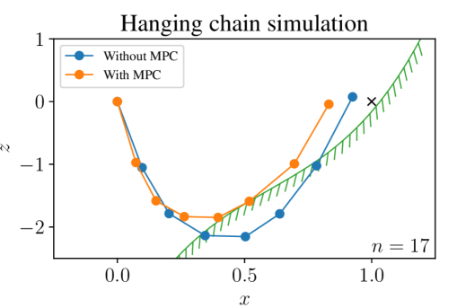
Figure 1: Snapshot of the MPC simulation of the hanging chain at time step 17, projected along the $y$-axis. The cubic state constraint is shown in green.

V-B Improvements to panoc

A total of six different solver configurations are compared: three solvers – the original panoc solver as described in [4], structured panoc using L–BFGS with inclusion of the Hessian-vector product in equation (12b), and structured panoc using L–BFGS without the rightmost term in (12b) – are all tested with the original line search condition and with the improved line search condition. The NMPC controller is simulated for 10 time steps, and the total number of function and gradient evaluations, the number of panoc iterations, and the run time are reported. A first experiment investigates the performance of the solvers when an initial guess of all zeros is used at each time step, whereas in a second experiment, the solver is warm-started using the solution and the Lagrange multipliers from the previous time step, shifted by one time step. The results are shown in Fig. 2.

Figure 2: Experimental results of the six solvers over 10 NMPC time steps of the chain model, first without warm-starting (top) and then warm-started using the shifted solution from the previous time step (bottom).

In most cases, the improved line search condition from Section IV reduces the number of function evaluations, the number of iterations, and the runtime. This is especially noticeable when the solver is cold-started.

When cold-started, the structured panoc solver with the Hessian-vector product of equation (12b) performs significantly better than standard panoc in terms of the number of iterations. However, the run time is similar. The reason for this is the Hessian-vector term in (12b), which requires an additional gradient evaluation in each iteration when using finite differences to compute this product. In the ideal case, standard panoc requires one gradient evaluation per iteration, whereas structured panoc with finite differences requires at least two, and this results in a higher run time per iteration.

The last two solvers approximate (12b) by dropping the Hessian-vector term entirely. This eliminates one gradient evaluation per iteration, which can clearly be seen in the figures. The number of iterations is very close to that of structured panoc with the Hessian-vector term, so dropping this term results in a significant reduction of the run time.

When warm-starting, the differences in the number of iterations between the six solvers are much smaller, but structured panoc without the Hessian-vector term still outperforms standard panoc. When including the Hessian-vector term, the number of gradient evaluations increases by almost a factor of two, as described above, resulting in a significantly worse run time.

V-C Comparison to Ipopt

In the following two experiments, the alpaqa implementation of structured panoc with the improved line search condition without Hessian-vector products (the best panoc-based solver from the previous subsection) is compared to the popular interior point solver Ipopt [1].

The tolerances used for alpaqa are $\varepsilon=\delta=10^{-3}$. For Ipopt, the tol and constr_viol_tol options are both set to $10^{-3}$. Three different configurations of Ipopt are used: (1) the default configuration with the exact Hessian without just-in-time compilation, (2) limited-memory Hessian approximation without just-in-time compilation, and (3) limited-memory Hessian approximation with just-in-time compilation. The four solvers are applied to the same hanging chain MPC problem as before and simulated for 30 time steps. In a first experiment, the solvers are not warm-started (initial guesses set to zero), and in a second experiment, all solvers are warm-started using the shifted solution and multipliers from the previous time step. The results are shown in Figure 3.

Figure 3: Comparison of the run time of alpaqa (approximate structured panoc with improved line search) and Ipopt (exact Hessian, limited memory Hessian, and limited memory with JIT compilation) for 30 optimal control problems (with and without warm starting).

It is clear that the alpaqa solver benefits from the warm start, being up to an order of magnitude faster compared to a cold start. Ipopt also converges slightly more quickly when warm-started, but the difference is not as substantial. Another observation is that the run time for Ipopt is relatively consistent across time steps, whereas the performance of alpaqa depends on the constraints: in the first iterations of the simulation, many state constraints are active, and more ALM iterations are required to satisfy them, at the end of the simulation, this is no longer the case, and alpaqa converges more quickly.

For smaller tolerances, Ipopt with the exact Hessian does have an advantage over the first-order alpaqa methods, but very precise solutions are usually not required in real-time MPC applications.

V-D Performance on the cutest benchmarks

When applied to a collection of 219 problems (excluding QPs) from the cutest benchmarks, the original panoc solver solves 148 problems, panoc with the improved line search condition solves 153, and structured panoc with the improved line search condition manages to solve 158. The latter is not only more robust, it also solves the problems more quickly than the original panoc solver, as shown in Figure 4.

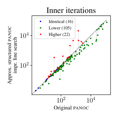
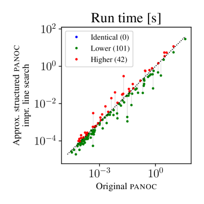
Figure 4: Comparison between the number of iterations and run time for the original panoc solver and the structured panoc solver with the improved line search, applied to cutest benchmarks.

VI Conclusion and further research

We presented the alpaqa library for nonconvex constrained optimization, and applied it to several benchmark problems. An attractive property of the augmented Lagrangian method and the panoc algorithm is that it can be warm-started, making it competitive with state-of-the-art solvers such as Ipopt in MPC applications. The use of first-order methods opens the door to large-scale problems and embedded environments.

The alpaqa library also implements two improvements to the original panoc algorithm: a way to compute the quasi-Newton steps while exploiting the structure of the box-constrained inner problems, and a stricter line search condition that can reject low-quality quasi-Newton steps. These modifications were shown to improve both the performance and the robustness of panoc.

Possible further work includes adding support for the quadratic penalty method for handling non-smooth constraints, implementing the second-order solution strategies covered in Sections III-A and III-B, and exploitation of the specific structure that arises from MPC problems.

References

- [1] Andreas Wächter and Lorenz T. Biegler “On the implementation of an interior-point filter line-search algorithm for large-scale nonlinear programming” In Mathematical Programming 106.1, 2006, pp. 25–57
- [2] Hande Y Benson and David F Shanno “Interior-point methods for nonconvex nonlinear programming: regularization and warmstarts” In Computational optimization and applications 40.2 Boston: Springer US, 2008, pp. 143–189
- [3] E.. Birgin and J.. Martínez “Practical Augmented Lagrangian Methods for Constrained Optimization” SIAM, 2014
- [4] L. Stella, A. Themelis, P. Sopasakis and P. Patrinos “A simple and efficient algorithm for nonlinear model predictive control” In 2017 IEEE 56th Annual Conference on Decision and Control (CDC), 2017, pp. 1939–1944 arXiv:1709.06487
- [5] Ajay Sathya et al. “Embedded nonlinear model predictive control for obstacle avoidance using PANOC” In 2018 European Control Conference (ECC), 2018, pp. 1523–1528 arXiv:1904.10546
- [6] Elias Small et al. “Aerial Navigation in Obstructed Environments with Embedded Nonlinear Model Predictive Control” In 2019 18th European Control Conference (ECC), 2019, pp. 3556–3563 arXiv:1812.04755
- [7] Pantelis Sopasakis, Emil Fresk and Panagiotis Patrinos “OpEn: Code Generation for Embedded Nonconvex Optimization” 21st IFAC World Congress In IFAC-PapersOnLine 53.2, 2020, pp. 6548–6554 arXiv:2003.00292
- [8] Joel A.. Andersson et al. “CasADi – A software framework for nonlinear optimization and optimal control” In Mathematical Programming Computation 11.1 Springer, 2019, pp. 1–36
- [9] R. Rockafellar and Roger J.-B. Wets “Variational analysis”, Grundlehren der mathematischen Wissenschaften 317 Berlin: Springer, 2004
- [10] Ben Hermans, Andreas Themelis and Panagiotis Patrinos “QPALM: A Proximal Augmented Lagrangian Method for Nonconvex Quadratic Programs”, 2020 arXiv:2010.02653
- [11] Dong C. Liu and Jorge Nocedal “On the limited memory BFGS method for large scale optimization” In Mathematical Programming 45.1-3 Springer-Verlag GmbHCo. KG, 1989, pp. 503–528
- [12] J.. Dennis and Jorge J. Moré “A Characterization of Superlinear Convergence and Its Application to Quasi-Newton Methods” In Mathematics of Computation 28.126 American Mathematical Society, 1974, pp. 549–560
- [13] Panagiotis Patrinos and Alberto Bemporad “Proximal Newton methods for convex composite optimization” In 52nd IEEE Conference on Decision and Control IEEE, 2013, pp. 2358–2363
- [14] Haw-Ren Fang and Dianne P O’Leary “Modified Cholesky algorithms: a catalog with new approaches” In Mathematical programming 115.2 Berlin/Heidelberg: Springer-Verlag, 2008, pp. 319–349
- [15] Jorge Nocedal and Stephen J. Wright “Numerical Optimization” New York: Springer, 2006
- [16] Iain Duff “MA57—a code for the solution of sparse symmetric definite and indefinite systems” In ACM transactions on mathematical software 30.2 NEW YORK: ACM, 2004, pp. 118–144
- [17] Andreas Themelis, Lorenzo Stella and Panos Patrinos “Forward-backward envelope for the sum of two nonconvex functions: further properties and nonmonotone line-search algorithms” In Siam Journal On Optimization 28.3 Society for IndustrialApplied Mathematics, 2018, pp. 2274–2303 arXiv:1606.06256
- [18] Leonard Wirsching, Hans Bock and Moritz Diehl “Fast NMPC of a chain of masses connected by springs” In Proceedings of the IEEE International Conference on Control Applications, 2006, pp. 591–596