Modeling ion beams, kinetic instabilities, and waves observed by the Parker Solar Probe near perihelia

Abstract

Recent in-situ observations from the Parker Solar Probe (PSP) mission in the inner heliosphere near perihelia show evidence of ion beams, temperature anisotropies, and kinetic wave activity, which are likely associated with kinetic heating and acceleration processes of the solar wind. In particular, the proton beams were detected by PSP/SPAN-I and related magnetic fluctuation spectra associated with ion-scale waves were observed by the FIELDS instrument. We present the ion velocity distribution functions (VDFs) from SPAN-I and the results of 2.5D and 3D hybrid-particle-in-cell (hybrid-PIC) models of proton and $\alpha$ particle super-Alfvénic beams that drive ion kinetic instabilities and waves in the inner-heliospheric solar wind. We model the evolution of the ion VDFs with beams, ion relative drifts speeds, and ion temperature anisotropies for solar wind conditions near PSP perihelia. We calculate the partition of energies between the particles (ions) along and perpendicular to the magnetic field, as well as the evolution of magnetic energy and compare to observationally deduced values. We conclude that the ion beam driven kinetic instabilities in the solar wind plasma near perihelia are important components in the cascade of energy from fluid to kinetic scale, an important component in the solar wind plasma heating process.

1 Introduction

It is well established that the dissipation of magnetized fluctuations in the solar wind occur at small kinetic scales below the ‘break point’ of the fluid-scale MHD turbulent cascade (see, e.g., recently Matteini et al., 2020; Bowen et al., 2020a) at frequencies near the proton gyro-resonance frequency. The ion kinetic instabilities in the inner heliospheric ($\leq 1$ AU) solar wind plasma could be driven by ion temperature anisotropy and ion beams in multi-ion solar winds (SW) plasma, as deduced in the past from the analysis of spacecraft data such as Wind (e.g., Kasper et al., 2008; Maruca et al., 2011, 2012; Alterman et al., 2018; Alterman & Kasper, 2019; Kasper & Klein, 2019), Helios (e.g., Marsch et al., 1982a, b; Hellinger et al., 2013; Ďurovcová et al., 2019b). Recent Parker Solar Probe observations substantiate this claim; for example, PSP Solar Wind Electrons Alphas & Protons (SWEAP) (Kasper et al., 2016) /Solar Probe Analyzers-Ions (SPAN-I) (Livi et al., 2021) VDFs and FIELDS (Bale et al., 2016) electromagnetic waves instrument observations show evidence that ion beams, kinetic instabilities and ion-scale waves play an important role in the dynamics of the SW plasma at never before explored perihelia regions (e.g. Verniero et al., 2020; Bowen et al., 2020a, b; Klein et al., 2021; Vech et al., 2021). The ion kinetic instabilities as evident from the non-Maxwellian ion VDFs, and the wave dispersion and dissipation, provide evidence in support for the heating at the dissipation scale as expected from the turbulent energy cascade theory from MHD fluid to small (kinetic) scales (e.g., Zank et al., 2018, 2021; Adhikari et al., 2021).

In coronal holes associated with the sources of the fast solar wind, the protons and ions are observed to be hotter than electrons and anisotropic, demonstrating the importance of anisotropic proton and heavier ion heating (e.g., Kohl et al., 1997; Cranmer et al., 1999; Hahn & Savin, 2013; Jeffrey et al., 2018). Moreover, $\alpha$ particles are typically hotter and faster than protons in the fast SW (e.g., Marsch et al., 1982b; Borovsky & Gary, 2014; Ďurovcová et al., 2019b, a) and could indicate the SW source regions (Ofman, 2004; Giordano et al., 2007; Ofman & Kramar, 2010; Abbo et al., 2016; Moses et al., 2020). The relative abundance of $\alpha$ particles in the solar wind varies considerably with the wind type and the solar cycle (e.g., Kasper et al., 2007; Ďurovcová et al., 2017; Alterman & Kasper, 2019). Analysis of spectroscopic observations shows that the heavy ion population may also become hotter and anisotropic in coronal streamers (e.g. Frazin et al., 2003; Abbo et al., 2016; Cranmer, 2020; Zhao et al., 2021) relevant to PSP measurements of the slow SW in the ecliptic plane.

In the present study we employ the well-established 2.5D and 3D hybrid modeling approach to study ion beams and related instabilities in electron-proton-$\alpha$ solar wind-like plasma developed by Ofman (2010) and Ofman et al. (2019), expanding on past methods (see Section 3 for details). The ion instabilities, nonlinear wave-particle interactions, and kinetic processes associated with the heating of ions are well described by the hybrid modeling approach, and the numerical noise is reduced to orders of magnitude below the modeled physical process level with adequate number of numerical particles, resolution, and well-tested numerical noise reduction techniques. Naturally, the purpose of the hybrid models is to focus on the SW parameter space where electrons can still be treated as a fluid. The nonlinear hybrid modeling approach uses the Particle-In-Cell (PIC) method for the ions, while electrons are treated as a background fluid through a generalized Ohms’ law. The model enables investigation of the observed self-consistent non-equilibrium ion VDFs, ion-scale wave spectra and the nonlinear dispersion relation. The advantage of this approach over other methods such as full-PIC is the computational cost effectiveness that is crucial for computationally demanding 3D modeling, where only ion kinetic timescales need to be resolved.

The hybrid models were used recently to model related multi-ion plasma instabilities in the SW; for example, the acceleration of protons and $\alpha$ particles by large amplitude Alfvén waves in the SW plasma was demonstrated using 1.5D hybrid model by Maneva et al. (2013). The effects of proton-$\alpha$ super-Alfvénic drift in inhomogeneous expanding solar wind was studied recently using 2.5D (Ofman et al., 2014; Maneva et al., 2015; Ozak et al., 2015; Ofman et al., 2017), as well as turbulence in solar wind at ion scales (Roberts & Ofman, 2019). Several 3D hybrid models of SW plasma were recently developed and applied primarily to study turbulence cascade to ion scales in SW plasma (e.g. Vasquez, 2015; Vasquez et al., 2020; Cerri et al., 2017; Franci et al., 2018; Hellinger et al., 2019; Markovskii et al., 2020). Recently, the nonlinear evolution of the proton-$\alpha$ drift instability and the $\alpha$ particle temperature anisotropy driven instability were modeled using the full 3D hybrid model (Ofman et al., 2019) for the expected parameters close to the Sun ($\sim 10R_{s}$), a region to be explored by PSP at perihelia (Encounters 22-24 in the years 2024-2025).

The present paper is the first multi-dimensional hybrid modeling nonlinear study of super-Alfvénic proton and the $\alpha$ particle beams and related instabilities in SW plasma. The paper is organized as follows. In Section 2 we discuss the PSP/SPAN-I and FIELDS instrument observation near perihelia that provide the observational motivation for our numerical study. In Section 3 we present the detail of the hybrid model. Section 4 is devoted to the numerical results, and Section 5 contains the discussion and conclusions, including the implications for PSP observations near perihelia.

2 Observational Motivations

The observational motivation for the present study is provided from PSP by the SPAN-I (Livi et al., 2021; Kasper et al., 2016) and FIELDS (Bale et al., 2016) instrument data. SPAN-I is a top-hat electrostatic analyzer that measures 3D ion velocity-space distributions and can separate protons from other heavy ions, such as $\alpha$ particles. Figure 1 shows an example wave event during PSP Encounter 4 (E4) at $\sim 36R_{s}$ on 26-Jan-2020 for the time period 13:50-14:55 UT. Panel (a) shows that the magnetic field B was nearly quiet and radially aligned. Wavelet analysis revealed in (b) that in the spacecraft frame, there was coherent ion-scale wave activity at $\sim$3 Hz (slightly above the proton gyrofrequency at $\sim 1$ Hz marked by the white dashed line), with a change in circular polarization signature from left-handed (blue) to right-handed (red) in panel (c). The waves appear at frequencies slightly larger than the proton gyro-frequency due to the (uncomputed) Doppler-shift from the plasma frame to the spacecraft frame. Note that the Doppler shift was not calculated due to previously discussed unresolved ambiguity (Verniero et al., 2020; Bowen et al., 2020b). The quantity $<S_{p}>$ indicates the degree of circular polarization, and $P_{tot}/P_{k}$ is the wave power normalized by background magnetic field fluctuations power. To extract wave power and polarization properties, we employ the Morlet wavelet transform to the FIELDS magnetometer data (Verniero et al., 2020; Bowen et al., 2020a; Torrence & Compo, 1998). Double bi-Maxwellian fits in (d) of the proton VDFs reveal that the beam-core drift speed (normalized by the Alfvén speed, $V_{A}$) may be regulating the wave-particle energy transfer process, as well as the proton temperature anisotropy of the core (red) and beam (blue) in (e). Other quantities that appear to qualitatively correlate with wave features are the preliminary plasma parameters obtained by the SPAN-I $\alpha$ particle moments, such as (f) $\alpha$-proton parallel (blue) and perpendicular (red) temperatures, (g) $\alpha$-proton drift speed normalized by $V_{A}$, and (h) $\alpha$-proton density ratio. To mitigate error due to SPAN-I partial field of view (FOV) obstruction by the heat shield, the $\alpha$ temperature anisotropy in Figure 1f was obtained by transforming the $\alpha$ particle temperature tensor to field-aligned-coordinates and extracting the perpendicular and parallel components. Here the overall $\alpha$ particle population produces $T_{\parallel}>T_{\perp}$, indicating a secondary $\alpha$ particle beam is present, as can be seen by the blue 1D VDF in Figure 2.

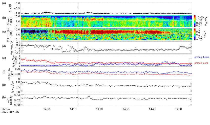
Figure 1: Example wave event at 36$R_{s}$ featuring a change in polarization from LH (blue) to RH (red). Shown is the (a) ratio of radial magnetic field component to total field magnitude, (b) wave power of B, (c) perpendicular polarization of B, (the white dash lines in (b) and (c) indicate the proton resonant frequency at $\sim 1$ Hz) (d) proton fits of beam-core drift speed, normalized by $V_{A}$, (e) proton temperature anisotropy fits of the core (red) and beam (blue), (f) $\alpha$ particle parallel (red) and perpendicular (blue) temperatures, (g) $\alpha$-proton drift speed, normalized by $V_{A}$, and (h) $\alpha$-proton density ratio.

From the SWEAP-I data it was found that most of the time $T_{\perp}/T_{\parallel}>1$ using bi-Maxwellian fits, as evident in Figure 1e. In the analysis of the VDF data, where the beam is subject to the beam instability and velocity space diffusion, the ion core and beam populations cannot be fully separated and evidently the fits provide larger $T_{\parallel}$ (than $T_{\perp}$) of the combined ion populations. In the hybrid model discussed below we model initially isotropic beam and core populations, and our model allows separating the populations unambiguously, following the time-dependent evolution of the beam and core VDFs and calculating the temperature anisotropies unambiguously using moments of the VDFs throughout the simulations.

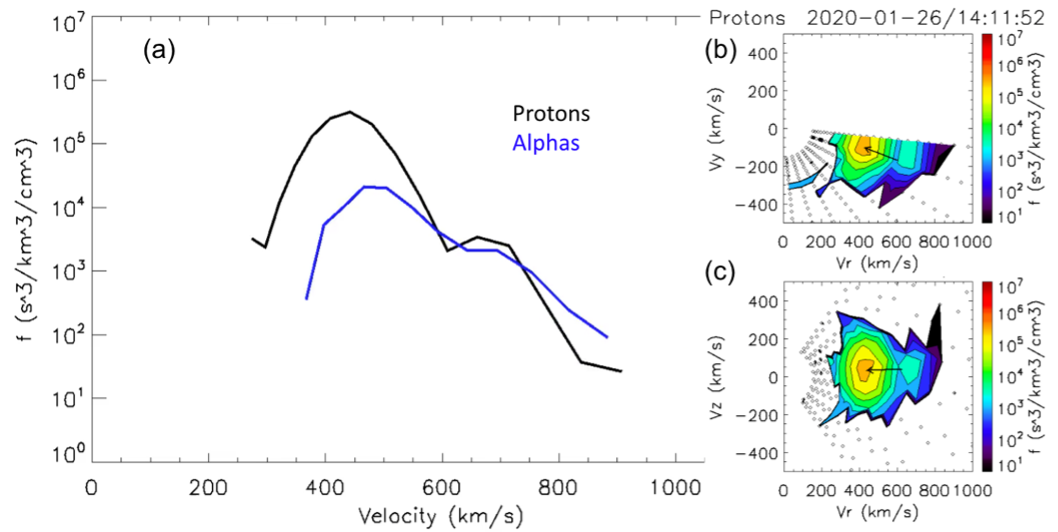
Figure 2: Example proton and $\alpha$ VDFs during wave event at time indicated by dashed black line in Figure 1. (a) VDF of protons (black) and $\alpha$ particles (blue), where all angles were summed and collapsed over energy. (b) Proton VDF contour elevation summed and collapsed onto azimuthal plane. (c) Proton VDF contour elevations summed and collapsed onto meridional plane. The black arrow indicates the direction of the magnetic field, where the arrowhead is at the solar wind velocity and the length is $V_{A}$.

Figure 2 shows an example of proton and $\alpha$ particle VDFs at the time indicated by the dashed black line in Figure 1. Shown in 2a are the 1D VDFs of protons (black) and $\alpha$ particles (blue) where the protons are exhibiting evidence of a bump-on-tail VDF. Panel 2b shows proton VDF contours in the azimuthal plane of the instrument, showing that the core of the distribution is sufficiently in the SPAN-I FOV. Panel 2c shows the VDF contours in the meridional plane, where we see two resolvable peaks in velocity space. Additional examples of proton beam VDFs at Encounters 4-8 can be found in Verniero et al. (2021), that show strong perpendicular spreading of the proton beam VDFs.

3 Hybrid-PIC Model, Boundary, and Initial Conditions

We use our recently developed parallelized 2.5D and 3D hybrid codes, based on the same principles as the 1D hybrid code originally developed by Winske & Omidi (1993), and later expanded to a 2.5D hybrid code (Ofman & Viñas, 2007) and parallelized by Ofman (2010) to model the proton-$\alpha$, magnetized SW plasma, recently extended to full 3D hybrid model (Ofman et al., 2019) (see the above references for details of the method of solution and the normalization). Here we mention briefly that the velocities are normalized by the proton Alfvén speed, $V_{A}$, the distances by the proton inertial length $\delta_{p}=c/\omega_{pp}$, where $\omega_{pp}$ is the proton plasma frequency), and the time is normalized by the inverse proton gyroresonat frequency $\Omega_{p}^{-1}$, where $\Omega_{p}=eB/m_{p}c$, where $B$ is the background magnetic field strength with $\mbox{\bf B}=B\mbox{\bf\^{x}}$, $m_{p}$ is the proton mass, and $c$ is the speed of light. Quasi-neutrality of the plasma is assumed, i.e., $n_{p}+2n_{\alpha}=n_{e}$, where $n_{p}$ is the proton number density, $n_{\alpha}$ is the $\alpha$ particle number density, and $n_{e}$ is the electron number density.

Ion kinetic dissipation scale is determined by the thermal proton gyroradius $r_{p}=V_{th,p}/\Omega_{p}$ or the ion inertial length $\delta_{p}$. These scales are typically of order $\lesssim$10 km in the solar wind at the distance of 36$R_{s}$ from the Sun using the measurements from PSP at E4 (e.g., Verniero et al., 2021). For example, the proton density at E4 was $\sim$1000 cm^-3, resulting in $\delta_{p}\sim 7$ km, while for proton temperature of 20 eV the thermal proton gyroradius is $r_{p}\sim 4$ km. The kinetic wave dissipation wavelength scale is typically an order of magnitude larger than $\delta_{p}$, as evident from the dispersion relation. The proton gyration is well resolved with the time step $0.02\Omega_{p}^{-1}$, and a ‘thermal’ proton travels $\sim 0.1\delta_{p}$ in one time step. The electron fluid equation in the model, i.e., the generalized Ohm’s law has the capability to include the resistive term. However, no resistivity was used in present model. Test with normalized empirical resistivity coefficient of $\eta=0.001$ did not affect the results.

The 2.5D hybrid codes solves three components of about $3.4\times 10^{7}$ particle velocities that are used to calculate the currents and the fields on the 2D spatial grid of $256\times 256$ cells with 512 particles per cell (ppc) and grid size 0.75$\delta_{p}$. Thus, the size of the computational domain is $(192\delta_{p})^{2}$. In the present study the 3D hybrid code uses $128^{3}$ cells with up to 128 ppc and grid size 1.5$\delta_{p}$ providing the 3D domain of $(192\delta_{p})^{3}$. We note that each numerical super-particle is modeled by a Gaussian charge distribution that is spread over several cells and represents many physical particles. In warm multi-ion plasma, the shortest length-scales to be resolved are determined by the ion kinetic dissipation scale. The solution of the Vlasov linear dispersion relation (e.g., Xie et al., 2004; Ofman & Viñas, 2007; Maneva et al., 2015; Verniero et al., 2020) shows that the proton and ion cyclotron waves are heavily damped at normalized $|k_{\parallel}|\gtrsim 1$ (normalized by $\delta_{p}^{-1}$). It is also evident from the linear Vlasov’s dispersion relation analysis (see, e.g., Stix, 1992; Verniero et al., 2020, Figure 9) that the fastest growing mode is well resolved. In Figure 3 we show the solution of the linear Vlasov’s dispersion relation for the proton beam parameters of Case 3 (see Table 1) for electron-proton plasma and parallel propagation. It is evident that the fastest growing mode is at $k_{\parallel,\gamma_{max}}=0.76$, and the corresponding growth rate is $\gamma_{max}=0.105\Omega_{p}^{-1}$. Thus, the linear growth stage of the instability is on the order of tens of gyroperiods. Increasing the beam relative density results in faster growth rate with somewhat shorter $k_{\parallel,\gamma_{max}}$ in the linear dispersion.

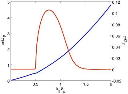
Figure 3: The linear Vlasov’s dispersion relation for the proton beam parameters in Case 3 (beam velocity magnitudes $V_{b,p}=2V_{A}$). The normalized real frequency $\omega$ (blue), and the growth rate $\gamma$ (red) dependence on $k_{\parallel}$ are shown. The fastest growing mode with $\gamma=0.105\Omega_{p}^{-1}$ is at $k_{\parallel}=0.76$.

Thus, our code resolves well the corresponding length scales down to the dissipation range and below, and the largest scale is more than an order of magnitude larger than the dissipation scale. The required number of particles per cell is determined by the limitation on the overall statistical noise, and the velocity space resolution which is typically a function of ion $\beta_{i}$. A numerical convergence test and total energy conservation monitoring were used to determine that the noise level is below the physical fluctuations level in the hybrid codes. The equation of the hybrid model and the details of the method of solution can be found in our past studies (Ofman & Viñas, 2007; Ofman et al., 2011, 2019). In the present study we employ periodic boundary conditions in an initially homogeneous $e-p-\alpha$ plasma. The hybrid model computes the self-consistent evolution of the ion VDFs and includes the nonlinear effects of wave-particle interactions without further simplifying assumptions and is well suited to describe the nonlinear saturated state and relaxation of the magnetized plasma ion kinetic instabilities. In the present study we have used the expanding box model (Grappin & Velli, 1996; Liewer et al., 2001) to model the solar wind gradual expansion with the expansion rate parameter $\epsilon=10^{-4}$, consistent with our previous studies (see, e.g., Ofman et al., 2011, 2017, 2019, for the expanding box model description, implemented in our 2.5D and 3D hybrid codes).

A self-consistent kinetic wave spectrum, produced by initially unstable (i.e., due to super-Alfvénic beams) plasma VDFs, is produced by the hybrid model (see below). Initial Maxwellian drifting ion populations lead to the drift instability for super-Alfvénic drift, resulting in non-Maxwellian VDFs in the nonlinear relaxed state in the nearly collisionless SW plasma. In Table 1 we list the various plasma parameters of the modeled cases in the present study.

Table 1: Plasma parameters of the numerical model runs for the various cases in the present study. The initial beam-core drift speed $V_{d0,p}$ for protons, the initial beam-core drift speed for $\alpha$ particles $V_{d0,\alpha}$, the initial proton core density $n_{p,c}$, the initial proton beam density $n_{p,b}$, the initial $\alpha$ core density $n_{\alpha,c}$, the initial $\alpha$ beam density $n_{\alpha,b}$, the $\beta$’s of the ion populations (defined in terms of $n_{e}$).

Case #	$V_{d0,p}$	$V_{d0,\alpha}$	$n_{p,c}$	$n_{p,b}$	$n_{\alpha,c}$	$n_{\alpha,b}$	$\beta_{p,c}$	$\beta_{p,b}$	$\beta_{\alpha,c}$	$\beta_{\alpha,b}$
1	2	2	0.819	0.091	0.03	0.015	0.429	0.0916	0.429	0.0916
2	2	2	0.728	0.182	0.03	0.015	0.429	0.0916	0.429	0.0916
3	2	0	0.9	0.1	0.045	-	0.429	0.0916	0.429	-
4	2.5	0	0.9	0.1	-	-	0.429	0.0916	-	-

In Figure 4 we show the initial state of the VDFs in the $V_{x}-V_{z}$ phase space plane for protons (Figure 4a-b) and $\alpha$ particles (Figure 4c-d) for Case 1. The cut along $V_{x}$ through the peak of the VDFs is shown in the lower panels. In all cases the proton and $\alpha$ particle beams are lower density and lower $\beta_{i}$ compared to the core ion populations, in qualitative agreement with examples of PSP SPAN-I observations. The super-Alfvénic drift speed between the beam and core is evident from the location of the peaks, the perpendicular temperatures and the relative number densities of the cores and beams are also evident from plots (1D cuts) of the 3D VDFs.

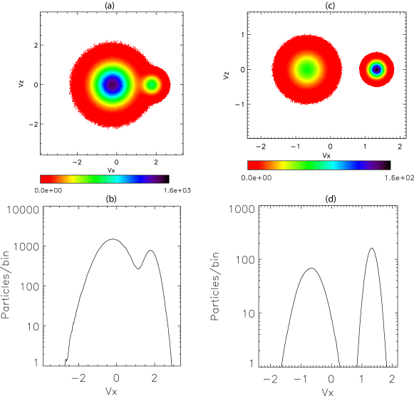
Figure 4: The initial state of the ion VDFs for Case 1 with beam velocity magnitudes $V_{b,p}=V_{b,\alpha}=2V_{A}$. The core populations are on the left and the beam populations are on the right in the center of mass frames. (a) The proton VDF in $V_{x}-V_{z}$ phase space plane. (b) The cut of the VDF along $V_{x}$ through the peak of the VDF shown in (a). (c) The $\alpha$ particle VDF in $V_{x}-V_{z}$ phase space plane. (d) The cut of the VDF along $V_{x}$ through the peak of the VDF shown in (c).

4 Numerical Results

In this section we present the results of the 2.5D and 3D hybrid modeling of the proton and $\alpha$ particle beams obtained from the 2.5D hybrid model, with parameters guided by PSP SPAN-I data. We show the evolutions of the ion VDFs, and the moments as evident in temperature anisotropies, parallel and perpendicular energies, and drift velocities of the various ion populations, as well as the associated magnetic energy and dispersions of the perpendicular magnetic fluctuations.

4.1 2.5D hybrid modeling results

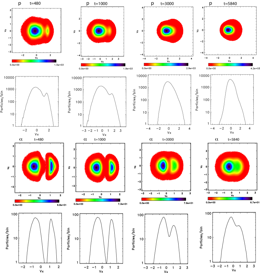
Figure 5: Top two panels: the proton VDFs for Case 1 in the $V_{x}-V_{z}$ phase space plane at $t=480$, $t=1000$, $t=3000$, and $t=5840$ $\Omega_{p}^{-1}$. Lower panels: the cuts of the proton VDFs along $V_{x}$ through the peaks of the distributions at the corresponding times. Lower two panels: the $\alpha$ particle VDFs for Case 1 in the $V_{x}-V_{z}$ phase space plane at $t=480$, $t=1000$, $t=3000$, and $t=5840$ $\Omega_{p}^{-1}$. The cuts of the $\alpha$ particle VDFs along $V_{x}$ through the peaks of the distributions at the corresponding times.

In Figures 5-11 we show the proton and $\alpha$ particle VDFs, the temporal evolution of the temperature anisotropies, the relative drift (beam) speed of the ion core and beam populations, and the associated magnetic energy and magnetic dispersion spectrum obtained from the 2.5D hybrid model. The proton VDFs at $t=480$, 1000, 3000, and 5840 $\Omega_{p}^{-1}$ with initial $\beta_{p,core}=0.429$, and a cold beam with initial $\beta_{p,beam}=0.092$, and with initial relative drift speed of $2V_{A}$ (Case 1) are shown in Figure 5. The upper panels show the proton VDFs in the $V_{x}-V_{z}$ phase space plane, and the lower panels show the cut of the VDFs along $V_{x}$ through the peak of the distributions at the corresponding times. The evolution and the structure of the non-Maxwellian core and beam VDFs are evident. The large temperature anisotropy (calculated from the ratio $T_{\perp}/T_{\parallel}$) of the beam population of protons is exhibited by the spread of the proton VDFs in $V_{z}$, with subsequent relaxation and merging of the core-beam proton population. The initial super-Alfvénic proton beam lead to the growth of magnetosonic instability, as expected from Vlasov’s linear stability analysis (see, e.g., Gary, 1993; Xie et al., 2004; Ofman & Viñas, 2007), with subsequent nonlinear saturation and relaxation. The linear growth stage of instability takes place within the first several tens of gyroperiods. After this short time the VDF of protons (as well as $\alpha$ particles) is no longer Maxwellian as evident in anisotropy increase in Figure 7 producing left-hand polarized resonant ion-cyclotron waves, evident in the dispersion relation resonant branches in Figure 10 below. The increased temperature anisotropy $T_{\perp}/T_{\parallel}>1$ of the ions leads to secondary ion-cyclotron instability driven primarily by the beam populations. The secondary instability is gradually damped due to wave-wave, wave-particle scattering, and velocity space diffusion into the parallel direction and absorption relaxation of the instability. The resulting gradual parallel heating of the ions is evident in Figure 8 below.

The $\alpha$ particle population VDFs at $t=480$, 1000, 3000, and 5840 $\Omega_{p}^{-1}$ for Case 1 with $n_{p,b}=0.092$ are shown in Figure 5 (lower two panels). The $\alpha$ particle VDFs in the $V_{x}-V_{z}$ phase space plane, and the lower panels show the cut of the $\alpha$ particle VDFs along $V_{x}$ through the peak of the $\alpha$ particle distributions at the corresponding times. The instability leads to rapid increase of the perpendicular anisotropy of the beam ion populations. This is followed by the isotropisation of the beam on much longer time scales, where the relaxation of the beam anisotropy of the $\alpha$ particle population proceeds more slowly compared to the proton population shown at the same time in Figure 5. Also, more gradual merging of the beam and the core $\alpha$ particle populations at the indicated times is evident. The very large (compared to protons) temperature anisotropy of the $\alpha$ particle beam population is exhibited by the wide spread of the $\alpha$ particle VDFs in $V_{z}$, with subsequent partial relaxation of the anisotropy and near-merging of the core-beam $\alpha$ particle population at $t=5840\ \Omega_{p}^{-1}$. The initial $\alpha$ particle super-Alfvénic beam results in the magnetosonic instability in the $\alpha$ particle population that proceeds together with the proton magnetosonic instability.

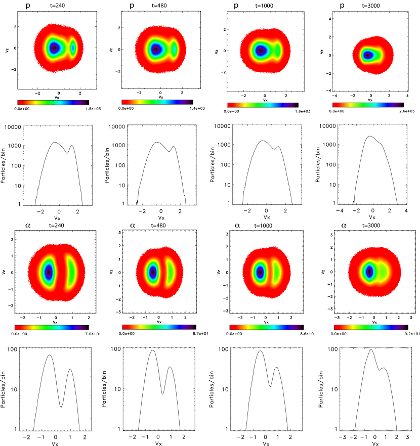
Figure 6: Top two panels: the proton VDFs for Case 2 in the $V_{x}-V_{z}$ phase space plane at $t=240$, $t=480$, $t=1000$, and $t=3000$ $\Omega_{p}^{-1}$. Lower panels: the cuts of the proton VDFs along $V_{x}$ through the peaks of the distributions at the corresponding times. Lower two panels: the $\alpha$ particle VDFs for Case 2 in the $V_{x}-V_{z}$ phase space plane at $t=240$, $t=480$, $t=1000$, and $t=3000$ $\Omega_{p}^{-1}$. The cuts of the $\alpha$ particle VDFs along $V_{x}$ through the peaks of the distributions at the corresponding times.

The proton VDFs $t=240$, 480, 1000, and 3000 $\Omega_{p}^{-1}$ for Case 2 with the same parameters as in Case 1 but with a twice denser beam population, $n_{p,b}=0.182$ are shown in Figure 6. The upper panels show the proton VDFs in the $V_{x}-V_{z}$ phase space plane, and the lower panels show the cut of the VDFs along $V_{x}$ through the peak of the distribution at the corresponding times. The more rapid (than in Case 1) growth and relaxation of the magnetosonic instability is evident. The large temperature anisotropy of the denser beam population of protons is exhibited by the spread of the proton VDFs in $V_{z}$, with subsequent rapid relaxation and merging of the core-beam proton population at $t=3000\ \Omega_{p}^{-1}$. Here as well, the initial proton super-Alfvénic beam results in the magnetosonic instability in the proton population, with subsequent nonlinear saturation and relaxation that proceeds more rapidly than in Case 1 (see, Figure 7 below).

The $\alpha$ particle population VDFs $t=240$, 480, 1000, and 3000 $\Omega_{p}^{-1}$ for Case 2 with $n_{p,b}=0.182$ are shown in Figure 6 (lower two panels). The $\alpha$ particle VDFs in the $V_{x}-V_{z}$ phase space plane is shown, and the lower panels show the cut of the $\alpha$ particle VDFs along $V_{x}$ through the peak of the $\alpha$ particle distributions at the corresponding times. The more rapid growth and relaxation of the magnetosonic instability in the $\alpha$ particle population compared to the proton population shown at the same time in Figure 6 is evident. The very large temperature anisotropy of the $\alpha$ particle beam population is exhibited by the wide spread of the $\alpha$ particle VDFs in $V_{z}$, with subsequent rapid relaxation and near-merging of the core-beam $\alpha$ particle population at $t=3000\ \Omega_{p}^{-1}$. Here as well, the initial $\alpha$ particle super-Alfvénic beam results in the magnetosonic instability in the $\alpha$ particle population, with subsequent nonlinear saturation that proceeds more rapidly than in the proton population.

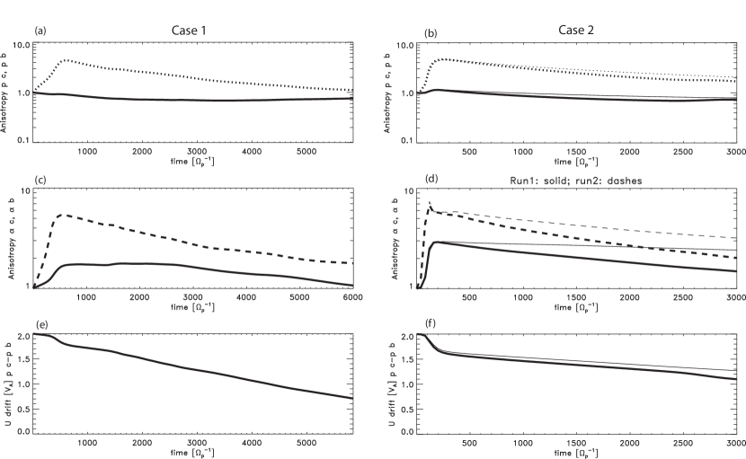
Figure 7: The temporal evolution of the temperature anisotropies and the proton beam-core drift speed $U_{drift}$ with initial drift speed $V_{d}=2V_{A}$ for Cases 1 and 2. The temperature anisotropies of the proton core (solid) and beam (dashes) populations for (a) Case 1 and (b) Case 2. The $\alpha$ particle core (solid) and beam (dashes) populations temperature anisotropies for (c) Case 1 and (d) Case 2. The $U_{drift}$ for (e) Case 1 and (f) Case 2. The corresponding quantities calculated without solar wind expansion are added for comparison for Case 2 (thin line styles).

The temporal evolution of the temperature anisotropy for the proton core and beam populations, the $\alpha$ particle core and beam populations, and the proton core-beam drift speeds, $U_{drift}$ for Cases 1 and 2 are shown for comparison in Figure 7. The more rapid growth and relaxation of the instability in Case 2 with $n_{p,b}=0.182$ than in Case 1 with $n_{p,b}=0.091$ is evident. The proton beam population temperature anisotropy in Case 1 peaks at $\sim 4.5$ at $t\approx 560\ \Omega_{p}^{-1}$, while in Case 2 the temperature anisotropy peaks at $\sim 5$ at $t\approx 230\ \Omega_{p}^{-1}$, with slight increase of the proton core population anisotropy. In Case 1 the $\alpha$ particle beam population reaches temperature anisotropy of $\sim 5.2$, while the $\alpha$ particle core population reaches temperature anisotropy of $\sim 1.8$. In Case 2 the $\alpha$ particle beam population reaches temperature anisotropy of $\sim 7$ at $t=110\ \Omega_{p}^{-1}$, while the $\alpha$ particle core population reaches temperature anisotropy of $\sim 3$. Thus, it is reasonable to conclude that the additional free energy in the proton beam produces more energetic wave spectrum that affects both, protons, and $\alpha$ particle populations. The temporal evolution of the moment of the proton parallel velocity $V_{x}$ of the core and beam populations shown, and the decrease of the drift speed due to the relaxation of the instability is apparent in Figures 7e-f, with more rapid evolution in Case 2 compared to Case 1. In order to demonstrate the effects of the gradual solar wind expansion on the evolution of the beam instability we have added the ion temperature anisotropies and the proton velocity drift calculated without solar wind expansion in Case 2. It is evident that expansion leads to more rapid decrease of the ion anisotropies and the proton drift velocity, and the effect of the expansion is more significant for the $\alpha$ particle populations compared to protons. In the proton core population there is a slight decrease of the proton core anisotropy to values $T_{\perp}/T_{\parallel}\lesssim 1$ after a couple of thousand gyroperiods in Cases 1 and 2 that is followed by slight increase of anisotropy back to $T_{\perp}/T_{\parallel}\sim 1$ that could be attributed to weak (slowly growing) firehose instability in the proton core population.

While it is evident that the proton-beam driven magnetosonic instability destabilizes the $\alpha$ particle population, we have evaluated the effects of the $\alpha$ particle beam instability by comparing the combined proton and $\alpha$ beam instabilities modeled in Case 1 to the proton only beam instability (i.e., without $\alpha$ particles) in Case 3. We found that the evolution of the proton instability is very similar to the evolution of the instability in Case 1, with slightly stronger effects of the solar wind expansion on the anisotropy decrease of the core proton population in Case 3 than in Case 1. This small difference could be attributed to the secondary heating of protons due to the $\alpha$ beam instability.

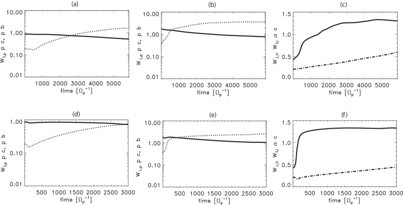
Figure 8: The temporal evolution of the parallel and perpendicular energies for Case 1 of (a) $W_{p,\parallel}$ of the proton core (solid) and beam (dashes) populations, (b) $W_{p,\perp}$ of the proton core (solid) and beam (dashes) population (c) $W_{\alpha,\perp}$ (solid) and $W_{\alpha,\parallel}$ (dot-dashes) of the $\alpha$ particle core population. (d)-(f) same as (a)-(c) for Case 2.

The temporal evolution of the parallel kinetic energy $W_{\parallel}$ and perpendicular kinetic energy $W_{\perp}$ for the proton and $\alpha$ particle populations for Case 1 and 2 are shown in Figure 8. The plots show that the parallel and perpendicular proton core energies change gradually in both cases, while the significant change takes place in the beam populations, consistent with the proton VDFs shown in Figures 5-6. The $W_{\parallel}$ of the proton beam population initially decreases, resulting in increased temperature anisotropy, shown in Figure 7a-b, with stronger effect in Case 2 compared to Case 1. The $W_{p,\parallel}$ decreases gradually in both cases with slight initial decrease of $W_{p,\parallel}$ in the proton beam population in Case 2, and corresponding increase of the $W_{p,\perp}$, followed by further gradual decrease as expected due to the gradual SW expansion. The $\alpha$ particle core $W_{\alpha,\perp}$ shows rapid increase due to the onset of the magnetosonic instability in Case 1 and 2 with more rapid increase in Case 2 compared to Case 1, consistent with the evolution of the $\alpha$ particle temperature anisotropy shown in Figure 7c-d.

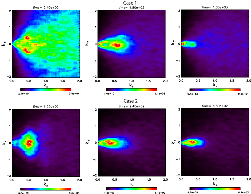
Figure 9: The $k$-plane power spectra of the perpendicular magnetic fluctuations due to the beam instabilities modeled in Cases 1 and 2 with the 2.5D hybrid code. The wavenumbers $k_{x}$, $k_{y}$ are normalized in units of $\delta_{p}^{-1}$. Top panels: Case 1 at $t=240$, 480, 1000 $\Omega_{p}^{-1}$. Lower panels: Case 2 at $t=120$, 240, 480 $\Omega_{p}^{-1}$.

In Figure 9 we show the $k$-plane power spectra of the perpendicular magnetic fluctuations due to the beam instabilities modeled in Cases 1 and 2 with the 2.5D hybrid code. In Case 1 it is evident that initially at the growth phase of the instability ($t=240\Omega_{p}^{-1}$) wave power is large in oblique modes at $k_{x}\approx 0.45\delta_{p}^{-1}$, $k_{y}\approx 0.4\delta_{p}^{-1}$ as well as in the parallel mode consistent with the linear Vlasov’s stability analysis at $k_{x}\approx 0.7\delta_{p}^{-1}$. The oblique modes damp, and the remaining wave power is in the unstable parallel mode, evident at $t=480\Omega_{p}^{-1}$. At later time, $t=1000\Omega_{p}^{-1}$ the unstable mode has damped, and only longer wavelength modes remain in the dissipation phase of the beam instability. Qualitatively similar evolution is evident in the more unstable Case 2, where at early time $t=120\Omega_{p}^{-1}$ the wave power is peaked near $k_{x}\approx 0.5\delta_{p}^{-1}$ with significant power in the oblique modes $|k_{y}|\lesssim 0.5$. At the later time $t=240\Omega_{p}^{-1}$ the oblique modes damp, and at $t=480\Omega_{p}^{-1}$ the remaining power is concentrated at the parallel mode, peaking at $k_{x}\approx 0.35\delta_{p}^{-1}$. It is evident that the power is concentrated in short wavelength wave, with typical $k~{}0.35-0.7\delta_{p}^{-1}$ corresponding the wavelengths in the range $9-18\delta_{p}$. With the PSP plasma parameters measured at E4 these values would correspond to wavelengths of 65-135 km in the solar wind rest frame.

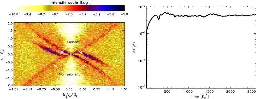
Figure 10: Left panel: The dispersion relation calculated from the 2.5D hybrid model of the Fourier-transformed spatial-temporal fluctuations of $B_{\perp}$ in Case 1 using the time interval $t=0-1024\ \Omega_{p}^{-1}$. The white arrows identify the resonant and noresonant branches. The intensity scale is logarithmic $(Log_{10})$

. Right panel: the temporal evolution of the integrated $|B_{\perp}|^{2}$ averaged over the computational domain, i.e., the normalized perpendicular magnetic energy density.

The dispersion relation calculated from the perpendicular magnetic fluctuations $B_{\perp}$ from the 2.5D hybrid model with the beam parameters of Case 1 is shown in Figure 10 (left panel). The various branches of the dispersion relation and the fastest growing modes identified as dark blue are evident. Comparing to the dispersion relations calculated from the 2.5D hybrid code (e.g., Xie et al., 2004; Ofman & Viñas, 2007; Ozak et al., 2015; Ofman et al., 2017), we can identify the resonant modes that show the largest intensities at $|k_{\parallel}|\sim 0.3$ and strong damping at $|k_{\parallel}|\gtrsim 1$, and the right-hand polarized non-resonant modes of weaker intensity appearing undamped at higher $\omega$ and $|k_{\parallel}|$ crossing and exceeding the proton gyroresonat frequencies $\omega=\pm\Omega_{p}$. The magnitude of the slope of the resonant branches is approximately $V_{A}$, as expected from the asymptotic stability threshold beam speed and their branches are shifted by about $0.5\Omega_{p}$ from the right-hand modes, indicating that these branches are produced by the $\alpha$ particle beam Doppler shifted with respect to the core population. It is interesting to note that the linear Vlasov’s dispersion (Figure 3) predicts higher $|k_{\parallel}|\sim 0.76$ for the fastest growing mode for the proton parameters of Case 1 and for $\alpha$ particles the peak growth is expected for half of this wavelength due to their smaller inertial length with respect to protons, i.e., $\delta_{\alpha}/\delta_{p}=(m_{\alpha}/m_{p})^{-1/2}=0.5$. Consistently, it is evident from the dispersion relation obtained with the hybrid model that the highest power of the resonant branches is in the range $|k_{\parallel}|\sim 0.3-0.7$.

The drifting population of the ions produces the Doppler shifted cyclotron resonances $\omega_{i}-k_{\parallel}V_{\parallel}=\Omega_{i}$ (e.g. Stix, 1962). While, both, the proton, and the $\alpha$ particle beam population resonances are shifted to higher frequencies, the $\alpha$ population may resonate with the $\alpha$ and proton-produced beam instability wave spectrum. Moreover, the $\alpha$ particle core population can affect the ion-cyclotron wave dispersion by introducing an absorption gap in the parallel-propagating waves (e.g. Cornwall & Schulz, 1971; Cuperman et al., 1988). Previous studies have considered proton-$\alpha$ population and ion population drift, rather than the proton-proton and $\alpha-\alpha$ beams of the present study, there are similarities in the dispersion wave spectra with the additional effects of the Doppler shift (see, e.g. Xie et al., 2004; Ofman et al., 2017). The average perpendicular magnetic energy $\left<|B_{\perp}|^{2}\right>$ shown in the right panel increase rapidly in time with the growth of the magnetosonic instability, following saturation at nearly constant level, consistent with the evolution of the instability and the ion temperature anisotropies for Case 1 shown in Figure 7a and c. The initial peak in $\left<|B_{\perp}|^{2}\right>$ can be associated with the peak of the $\alpha$ beam temperature anisotropy evident in Figure 7d, and the relaxation of the $\alpha$ population beam-driven instability.

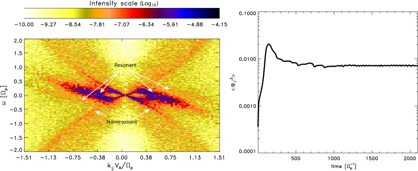
Figure 11: Same as Figure 10 for Case 2.

The dispersion relation calculated from the perpendicular magnetic fluctuations $B_{\perp}$ from the 2.5D hybrid model with the beam parameters of Case 2 is shown in Figure 11 (left panel). Here as well, the branches of the dispersion relation and the fastest growing modes identified as dark blue are evident. The more energetic, faster growing instability in Case 2 results in stronger wave activity compared to Case 1 as evident from the more extensive high intensity (blue) regions in the dispersion relation branches showing evidence of both, $\alpha$ and weaker proton branches. Comparing the dispersion relation to Case 1 and the previous studies mentioned above, we can identify the resonant modes that show the largest intensity in the range $|k_{\parallel}|\sim 0.1-0.8$ and strong damping for $|k_{\parallel}|>1$, while the non-resonant modes of weaker intensity proceed undamped at higher $\omega$ exceeding the proton gyroresonat frequency. The $\alpha$ particle branches are evident with an approximate slope magnitude of $V_{A}$, the asymptotic stability threshold, and shifted by about $0.5\Omega_{p}$ with respect to the non-resonant branches, with apparent Doppler-shifted proton branches at higher frequencies. However, the combined effects of power obtained from the nonlinear evolution of the ion resonances on the dispersion spectrum is not well separable in the present case. The total perpendicular magnetic energy increases rapidly with the growth of the magnetosonic instability within $\sim 110\omega_{p}^{-1}$, following rapid decrease and saturation at nearly constant level, consistent with the evolution of the instability and the ion temperature anisotropies for Case 2 shown in Figure 7b and d.

4.2 3D hybrid modeling results

Figures 12-13 show the results of the 3D hybrid modeling for Case 4 with an initial proton beam speed of 2.5$V_{A}$ with respect to the core. The number density of the beam is 10% of the total proton population, with 90% of the protons in the core. It is evident in Figure 12 that the initial Maxwellian VDF of the beam becomes anisotropic with increased $T_{p,\perp}$, marked by the spread of the beam VDF in the perpendicular ($V_{z}$) direction at $t=80$, and 200 $\Omega_{p}^{-1}$. The proton core VDF remains nearly Maxwellian at this relatively short timescale (compared to the 2.5D runs in Cases 1-3).

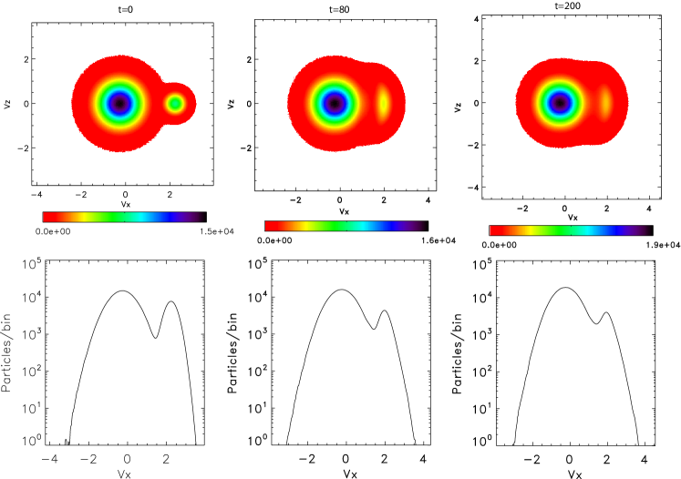
Figure 12: The VDFs obtained from the 3D hybrid model for Case 4 with $V_{d}=2.5V_{A}$. The top panels show the proton VDFs in the $V_{x}-V_{z}$ phase space plane in the initial state (t=0) and at $t=80$, and 200 $\Omega_{p}^{-1}$. The lower panels show the cut along $V_{x}$ through the peak of the VDFs.

The temporal evolution of the proton core and beam populations temperature anisotropies, and the proton beam-core drift speed $U_{drift}$ for Case 4 is shown in Figure 13. The initial growth of the beam-driven magnetosonic instability results in increase of the temperature anisotropy to $4.3$ within $\sim 32$ $\Omega_{p}^{-1}$, with subsequent decrease to $3.3$ at $t=200\ \Omega_{p}^{-1}$. The corresponding initially rapid decrease of the beam-core drift speed is evident, followed by gradual decrease. The core proton population remains nearly isotropic throughout the modeled evolution to $t=200\ \Omega_{p}^{-1}$, with very gradual decrease, with contribution to the decrease by the solar wind expansion, where the expansion parameter was set at $\epsilon=10^{-4}$ in the 3D hybrid model (same as used in the 2.5D hybrid model).

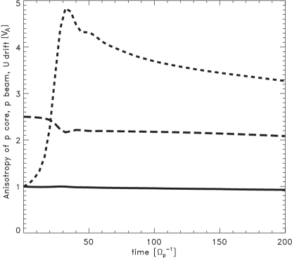
Figure 13: The temporal evolution of the proton core population temperature anisotropy (solid), proton beam population temperature anisotropy (short dashes) and the core-beam drift speed $U_{drift}$ (long dashes) obtained from the 3D hybrid model for Case 4 with $V_{d}=2.5V_{A}$.

In order to evaluate the importance of the 3D effects on the evolution of the proton beam-driven magnetosonic instability, we have compared the 3D hybrid model results to the results of 2.5D hybrid model with otherwise identical physical and numerical parameters. We found that the temporal evolution of the temperature anisotropies and relaxation rate of the instability in the 3D model is close to the 2.5D model, and the results of the two models are similar. The main difference is slightly faster onset and initial growth of the instability in 2.5D hybrid model compared to the 3D hybrid model result, where the peak temperature anisotropy of the beam is reached $\sim 10\ \Omega_{p}^{-1}$ sooner than in 3D hybrid model, but, reaching close maximal proton beam temperature anisotropy of $\sim 4$ in the two models.

5 Discussion and Conclusions

Recent PSP SPAN-I observations near perihelia find evidence of proton and $\alpha$ particles non-Maxwellian VDFs with core and beam populations, with FIELDS instrument detecting related periods of high ion-scale wave activity in the solar wind plasma at PSP perihelia (Encounter 4) with further observations of proton beams in Encounters 4-8 (Verniero et al., 2020, 2021). Motivated by PSP observations, we use 2.5D and 3D expanding box hybrid modeling to investigate the growth and nonlinear state of the instabilities and kinetic waves produced by proton and $\alpha$ beams, and a temperature anisotropy using hybrid simulations. The parameters of the models such as ion $\beta_{\parallel}$ and the core-beam super-Alfvénic differential speed are guided by the PSP ion data. We find good qualitative agreement between the modeled VDFs and the proton PSP SPAN-I observations, that show similar core-beam bump-on-tail structure for protons and $\alpha$ particles. The modeled dispersion of the ion-scale waves and the $k$-spectrum evolution show strong power in ion scale waves identified in the model as resonant ion-cyclotron and non-resonant magnetosonic waves. The PSP FIELD instrument has provided evidence of periods of ion-scale wave activity with left-hand and right-hand polarization, in qualitative agreement with the model results. However, direct comparison to the PSP/FIELDS observations obtained in the spacecraft frame to the results in the solar wind frame that model the evolution of a particular plasma parcel, are ambiguous due to the effects of Doppler shift, and the possible variation of the solar wind plasma properties (possibly unrelated to the evolution of the beam instability) as it flows by the spacecraft detectors. The hybrid models show that super-Alfvénic beams lead to rapid (in terms of $\Omega_{p}^{-1}$) growth of the magnetosonic instability and in agreement with Vlasov’s linear theory, reaching quickly the nonlinear saturated state, with significant temperature anisotropy increase of the proton and $\alpha$ particle beam populations (peaking at $\sim 4$ for the modeled parameters), and with smaller anisotropy of the core populations, followed by gradual relaxation of the drift and anisotropies. We note that the peak anisotropies for the proton beam in Case 1 of the model exceed 4 for about 400 gyroperiods ($\sim 4$ min) and for 250 gyroperiods ($\sim$2.5 min) in Case 2, with most of the modeled evolution time of several thousand gyroperiods in agreement with the range of anisotropies obtained from PSP observations. The PSP data in Figure 1 show anisotropies as high as  4 at t=13:50-13:52 and 14:44-14:45 comparable to the peak anisotropies in the model.

We find that the instability growth rate and nonlinear saturation level of the temperature anisotropy and magnetic wave energy increase with the proton beam population density. The initial growth stage takes place within several tens of proton gyroperiods as predicted by linear theory, and relaxation of the instability occurs over several thousand gyroperiods with the beam protons eventually merging with the core proton populations through phase-space diffusion, combined with a small effect of perpendicular temperature decrease due to SW expansion, in agreement with previous studies. The $\alpha$ particle population shows faster growth of the instability for the same beam speed and more gradual relaxation than protons of the beam-driven instability. This is due to the combined effects of the larger $\alpha$ beam-to-core density ratio and the absorption of some of the proton-beam produced wave-spectrum energy Doppler shifted to the resonant frequency range, as evident in the dispersion relation. While the interaction between the proton and $\alpha$ beams is not strong due to their separation in the wave dispersion, some of the proton instability produced wave spectrum is absorbed by the $\alpha$ particles due to the Doppler shift of the beam populations. The perpendicular heating of the ions leads to a secondary instability driven by their temperature anisotropy. We extend the hybrid model of the proton-beam driven instability to the full 3D expanding box model and find similar results as in the 2.5D hybrid model for the same physical parameters, indicating that the main effects of the growth and saturation of the instability are due to the parallel and planar propagating waves. Both the 2.5D and 3D hybrid models produce the 3D VDFs of protons and $\alpha$ particles that are in qualitatively good agreement PSP SPAN-I observations.

The LJ and LO acknowledge support by NASA LWS grant 80NSSC20K0648. LO acknowledges support by NASA Cooperative Agreement NNG11PL10A to The Catholic University of America, and NASA Partnership for Heliophysics and Space Environment Research (PHaSER) award 80NSSC21M0180. JV and DL acknowledge the support by NASA contract NNN06AA01C. We thank Michael McManus for the help in producing Figures 1 and 2. We thank the PSP mission team for generating the data and making them publicly available. Resources supporting this work were provided by the NASA High-End Computing (HEC) Program through the NASA Advanced Supercomputing (NAS) Division at Ames Research Center. The authors thank Dr. Vadim Roytershtein for providing the linear Vlasov dispersion solver.

References

- Abbo et al. (2016) Abbo, L., Ofman, L., Antiochos, S. K., et al. 2016, Space Sci. Rev., 201, 55, doi: 10.1007/s11214-016-0264-1
- Adhikari et al. (2021) Adhikari, L., Zank, G. P., Zhao, L. L., Nakanotani, M., & Tasnim, S. 2021, A&A, 650, A16, doi: 10.1051/0004-6361/202039297
- Alterman & Kasper (2019) Alterman, B. L., & Kasper, J. C. 2019, ApJ, 879, L6, doi: 10.3847/2041-8213/ab2391
- Alterman et al. (2018) Alterman, B. L., Kasper, J. C., Stevens, M. L., & Koval, A. 2018, ApJ, 864, 112, doi: 10.3847/1538-4357/aad23f
- Bale et al. (2016) Bale, S. D., Goetz, K., Harvey, P. R., et al. 2016, Space Sci. Rev., 204, 49, doi: 10.1007/s11214-016-0244-5
- Borovsky & Gary (2014) Borovsky, J. E., & Gary, S. P. 2014, Journal of Geophysical Research (Space Physics), 119, 5210, doi: 10.1002/2014JA019758
- Bowen et al. (2020a) Bowen, T. A., Bale, S. D., Bonnell, J. W., et al. 2020a, ApJ, 899, 74, doi: 10.3847/1538-4357/ab9f37
- Bowen et al. (2020b) Bowen, T. A., Mallet, A., Bale, S. D., et al. 2020b, Phys. Rev. Lett., 125, 025102, doi: 10.1103/PhysRevLett.125.025102
- Cerri et al. (2017) Cerri, S. S., Servidio, S., & Califano, F. 2017, ApJ, 846, L18, doi: 10.3847/2041-8213/aa87b0
- Cornwall & Schulz (1971) Cornwall, J. M., & Schulz, M. 1971, J. Geophys. Res., 76, 7791, doi: 10.1029/JA076i031p07791
- Cranmer (2020) Cranmer, S. R. 2020, ApJ, 900, 105, doi: 10.3847/1538-4357/abab04
- Cranmer et al. (1999) Cranmer, S. R., Field, G. B., & Kohl, J. L. 1999, ApJ, 518, 937, doi: 10.1086/307330
- Cuperman et al. (1988) Cuperman, S., Ofman, L., & Dryer, M. 1988, J. Geophys. Res., 93, 2533, doi: 10.1029/JA093iA04p02533
- Franci et al. (2018) Franci, L., Landi, S., Verdini, A., Matteini, L., & Hellinger, P. 2018, ApJ, 853, 26, doi: 10.3847/1538-4357/aaa3e8
- Frazin et al. (2003) Frazin, R. A., Cranmer, S. R., & Kohl, J. L. 2003, ApJ, 597, 1145, doi: 10.1086/378558
- Gary (1993) Gary, S. P. 1993, Theory of Space Plasma Microinstabilities (Cambridge University Press, New York, NY)
- Giordano et al. (2007) Giordano, S., Fineschi, S., Ofman, L., Mancuso, S., & Abbo, L. 2007, in ESA Special Publication, Vol. 641, Second Solar Orbiter Workshop, ed. E. Marsch, K. Tsinganos, R. Marsden, & L. Conroy, 31
- Grappin & Velli (1996) Grappin, R., & Velli, M. 1996, J. Geophys. Res., 101, 425, doi: 10.1029/95JA02147
- Hahn & Savin (2013) Hahn, M., & Savin, D. W. 2013, ApJ, 776, 78, doi: 10.1088/0004-637X/776/2/78
- Hellinger et al. (2019) Hellinger, P., Matteini, L., Landi, S., et al. 2019, ApJ, 883, 178, doi: 10.3847/1538-4357/ab3e01
- Hellinger et al. (2013) Hellinger, P., TráVníček, P. M., Štverák, Š., Matteini, L., & Velli, M. 2013, Journal of Geophysical Research (Space Physics), 118, 1351, doi: 10.1002/jgra.50107
- Jeffrey et al. (2018) Jeffrey, N. L. S., Hahn, M., Savin, D. W., & Fletcher, L. 2018, ApJ, 855, L13, doi: 10.3847/2041-8213/aab08c
- Kasper & Klein (2019) Kasper, J. C., & Klein, K. G. 2019, ApJ, 877, L35, doi: 10.3847/2041-8213/ab1de5
- Kasper et al. (2008) Kasper, J. C., Lazarus, A. J., & Gary, S. P. 2008, Physical Review Letters, 101, 261103, doi: 10.1103/PhysRevLett.101.261103
- Kasper et al. (2007) Kasper, J. C., Stevens, M. L., Lazarus, A. J., Steinberg, J. T., & Ogilvie, K. W. 2007, ApJ, 660, 901, doi: 10.1086/510842
- Kasper et al. (2016) Kasper, J. C., Abiad, R., Austin, G., et al. 2016, Space Sci. Rev., 204, 131, doi: 10.1007/s11214-015-0206-3
- Klein et al. (2021) Klein, K. G., Verniero, J. L., Alterman, B., et al. 2021, ApJ, 909, 7, doi: 10.3847/1538-4357/abd7a0
- Kohl et al. (1997) Kohl, J. L., Noci, G., Antonucci, E., et al. 1997, Sol. Phys., 175, 613, doi: 10.1023/A:1004903206467
- Liewer et al. (2001) Liewer, P. C., Velli, M., & Goldstein, B. E. 2001, J. Geophys. Res., 106, 29261, doi: 10.1029/2001JA000086
- Livi et al. (2021) Livi, R., Larson, D. E., Kasper, J. C., et al. 2021, Earth and Space Science Open Archive, 20, doi: 10.1002/essoar.10508651.1
- Maneva et al. (2015) Maneva, Y. G., Ofman, L., & Viñas, A. 2015, A&A, 578, A85, doi: 10.1051/0004-6361/201424401
- Maneva et al. (2013) Maneva, Y. G., ViñAs, A. F., & Ofman, L. 2013, Journal of Geophysical Research (Space Physics), 118, 2842, doi: 10.1002/jgra.50363
- Markovskii et al. (2020) Markovskii, S. A., Vasquez, B. J., & Chandran, B. D. G. 2020, ApJ, 889, 7, doi: 10.3847/1538-4357/ab5af3
- Marsch et al. (1982a) Marsch, E., Rosenbauer, H., Schwenn, R., Muehlhaeuser, K., & Neubauer, F. M. 1982a, J. Geophys. Res., 87, 35, doi: 10.1029/JA087iA01p00035
- Marsch et al. (1982b) Marsch, E., Rosenbauer, H., Schwenn, R., Muehlhaeuser, K. H., & Neubauer, F. M. 1982b, J. Geophys. Res., 87, 35, doi: 10.1029/JA087iA01p00035
- Maruca et al. (2011) Maruca, B. A., Kasper, J. C., & Bale, S. D. 2011, Physical Review Letters, 107, 201101, doi: 10.1103/PhysRevLett.107.201101
- Maruca et al. (2012) Maruca, B. A., Kasper, J. C., & Gary, S. P. 2012, ApJ, 748, 137, doi: 10.1088/0004-637X/748/2/137
- Matteini et al. (2020) Matteini, L., Franci, L., Alexandrova, O., et al. 2020, Frontiers in Astronomy and Space Sciences, 7, 83, doi: 10.3389/fspas.2020.563075
- Moses et al. (2020) Moses, J. D., Antonucci, E., Newmark, J., et al. 2020, Nature Astronomy, 4, 1134, doi: 10.1038/s41550-020-1156-6
- Ofman (2004) Ofman, L. 2004, Advances in Space Research, 33, 681, doi: 10.1016/S0273-1177(03)00235-7
- Ofman (2010) —. 2010, Journal of Geophysical Research (Space Physics), 115, A04108, doi: 10.1029/2009JA015094
- Ofman et al. (2019) Ofman, L., Koval, A., Wilson, L. B., & Szabo, A. 2019, J. Geophys. Res., 124, 2393, doi: 10.1029/2018JA026301
- Ofman & Kramar (2010) Ofman, L., & Kramar, M. 2010, in Astronomical Society of the Pacific Conference Series, Vol. 428, SOHO-23: Understanding a Peculiar Solar Minimum, ed. S. R. Cranmer, J. T. Hoeksema, & J. L. Kohl, 321. https://arxiv.org/abs/1004.4847
- Ofman & Viñas (2007) Ofman, L., & Viñas, A. F. 2007, J. Geophys. Res., 112, 6104, doi: 10.1029/2006JA012187
- Ofman et al. (2014) Ofman, L., Viñas, A. F., & Maneva, Y. 2014, Journal of Geophysical Research (Space Physics), 119, 4223, doi: 10.1002/2013JA019590
- Ofman et al. (2011) Ofman, L., Viñas, A. F., & Moya, P. S. 2011, Annales Geophysicae, 29, 1071, doi: 10.5194/angeo-29-1071-2011
- Ofman et al. (2017) Ofman, L., Viñas, A. F., & Roberts, D. A. 2017, Journal of Geophysical Research (Space Physics), 122, 5839, doi: 10.1002/2016JA023705
- Ozak et al. (2015) Ozak, N., Ofman, L., & Viñas, A. F. 2015, ApJ, 799, 77, doi: 10.1088/0004-637X/799/1/77
- Roberts & Ofman (2019) Roberts, D. A., & Ofman, L. 2019, Sol. Phys., 294, 153, doi: 10.1007/s11207-019-1548-x
- Stix (1962) Stix, T. H. 1962, The Theory of Plasma Waves (New York et al.: McGraw-Hill Book Co.)
- Stix (1992) —. 1992, Waves in plasmas (American Institute of Physics, New York, NY)
- Torrence & Compo (1998) Torrence, C., & Compo, G. P. 1998, Bulletin of the American Meteorological Society, 79, 61 , doi: 10.1175/1520-0477(1998)079<0061:APGTWA>2.0.CO;2
- Vasquez (2015) Vasquez, B. J. 2015, ApJ, 806, 33, doi: 10.1088/0004-637X/806/1/33
- Vasquez et al. (2020) Vasquez, B. J., Isenberg, P. A., & Markovskii, S. A. 2020, ApJ, 893, 71, doi: 10.3847/1538-4357/ab7e2b
- Ďurovcová et al. (2019a) Ďurovcová, T., Němeček, Z., & Šafránková, J. 2019a, ApJ, 873, 24, doi: 10.3847/1538-4357/ab01c8
- Ďurovcová et al. (2019b) Ďurovcová, T., Šafránková, J., & Němeček, Z. 2019b, Sol. Phys., 294, 97, doi: 10.1007/s11207-019-1490-y
- Ďurovcová et al. (2017) Ďurovcová, T., Šafránková, J., Němeček, Z., & Richardson, J. D. 2017, ApJ, 850, 164, doi: 10.3847/1538-4357/aa9618
- Vech et al. (2021) Vech, D., Martinović, M. M., Klein, K. G., et al. 2021, A&A, 650, A10, doi: 10.1051/0004-6361/202039296
- Verniero et al. (2020) Verniero, J. L., Larson, D. E., Livi, R., et al. 2020, ApJS, 248, 5, doi: 10.3847/1538-4365/ab86af
- Verniero et al. (2021) Verniero, J. L., Chandran, B. D. G., Larson, D. E., et al. 2021, arXiv e-prints, arXiv:2110.08912. https://arxiv.org/abs/2110.08912
- Winske & Omidi (1993) Winske, D., & Omidi, N. 1993, Computer Space Plasma Physics: Simulation Techniques and Sowftware, H. Matsumoto and Y. Omura (eds.) (Terra SP, Tokyo), 103–160
- Xie et al. (2004) Xie, H., Ofman, L., & ViñAs, A. 2004, Journal of Geophysical Research (Space Physics), 109, A08103, doi: 10.1029/2004JA010501
- Zank et al. (2018) Zank, G. P., Adhikari, L., Hunana, P., et al. 2018, ApJ, 854, 32, doi: 10.3847/1538-4357/aaa763
- Zank et al. (2021) Zank, G. P., Zhao, L. L., Adhikari, L., et al. 2021, Physics of Plasmas, 28, 080501, doi: 10.1063/5.0055692
- Zhao et al. (2021) Zhao, J., Gibson, S. E., Fineschi, S., et al. 2021, ApJ, 912, 141, doi: 10.3847/1538-4357/abf143