Unsupervised Domain Generalization by Learning a Bridge Across Domains

Abstract

The ability to generalize learned representations across significantly different visual domains, such as between real photos, clipart, paintings, and sketches, is a fundamental capacity of the human visual system. In this paper, different from most cross-domain works that utilize some (or full) source domain supervision, we approach a relatively new and very practical Unsupervised Domain Generalization (UDG) setup of having no training supervision in neither source nor target domains. Our approach is based on self-supervised learning of a Bridge Across Domains (BrAD) - an auxiliary bridge domain accompanied by a set of semantics preserving visual (image-to-image) mappings to BrAD from each of the training domains. The BrAD and mappings to it are learned jointly (end-to-end) with a contrastive self-supervised representation model that semantically aligns each of the domains to its BrAD-projection, and hence implicitly drives all the domains (seen or unseen) to semantically align to each other. In this work, we show how using an edge-regularized BrAD our approach achieves significant gains across multiple benchmarks and a range of tasks, including UDG, Few-shot UDA, and unsupervised generalization across multi-domain datasets (including generalization to unseen domains and classes).

1 Introduction

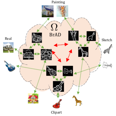
Figure 1: Originally, same domain instances are closer to each other than to instances of the same class in other domains. Naive application of popular self-supervised learning techniques tends to separate domains before classes (Section 4). Our approach is to learn a BrAD - an auxiliary bridge domain (e.g. of edge-like images) that helps aligning instances of the same class across domains. Arrows indicate forces in feature space applied by our training losses (Section 3). green = attraction; red = repulsion.

When observing some technical manual with schematic drawings of equipment for the first time, people do not need any supervision to associate these schematic drawings to real complex objects. This demonstrates the importance and efficiency of one of the basic human capacities - ability to learn with little to no supervision across multiple visual domains, as well as to effectively generalize to new domains and even new object classes without additional supervision.

Recent literature, extensively discussed in Section 2, is rich in works on learning to semantically generalize across domains without supervision in the target domain(s). The target domains can be observed as a collection of unlabeled images in Unsupervised Domain Adaptation (UDA), or even completely unseen during training in Domain Generalization (DG). For both UDA and DG, success in generalization would mean that the desired downstream tasks (classification, detection, etc.) would successfully transfer to a new seen or unseen domain. However, in most UDA and DG works an abundant source domain supervision for the intended downstream task is assumed. But do we always have that in real-life use-cases? In many situations, such as in the technical manuals example above, we need our systems to generalize not only to new domains, but also to completely new kinds of objects for which we might have very little data (images and/or labels) - not sufficient to train the standard UDA or DG methods. Few recent Unsupervised DG (UDG) and Few-Shot UDA (FUDA) works, realized the importance of this issue, and restrict the source domain(s) supervision to few or even zero labeled examples. In this paper we target the least restrictive (in terms of labeling requirements) UDG setting, where we do not require any source domain supervision at training, and which also implicitly supports generalization to completely new unseen visual domains with new unseen classes.

We all draw an edge-like image when asked to draw something quickly. Object edges seems to be our shared universal visual representation for all the domains we observe. This drove the basic intuition behind our BrAD approach: teach the machine to represent all the visual domains (in feature space) in the same way as it represents this seemingly universally shared visual domain of edge-like images. Our approach (Figure 1) is based on our proposed concept of a learnable Bridge Across Domains (BrAD) - an auxiliary visual ‘bridge’ domain to which it is relatively easy to visually map (in an image-to-image sense) all the domains of interest. The BrAD is used only during contrastive self-supervised training of our model for semantically aligning the representations (features) of each of the training domains to the ones for the shared BrAD. By transitivity of this semantic alignment in feature space, the learned model representations for all the domains are all BrAD-aligned and hence implicitly aligned to each other. This makes the learned mappings to the BrAD unnecessary for inference, making the trained model generalize-able even to new unseen domains (for which we do not have BrAD mappings) at test time. Moreover, not depending on BrAD-mapping for inference allows exploiting additional non-BrAD-specific features (e.g. color) which are also learned by our representation model encoder (Sec. 3). We show that even a simple heuristic implementation of the BrAD idea, mapping images to their edge maps, already gives a nice improvement over strong self-supervised baselines not utilizing BrAD. We further show that with learnable BrAD, our method demonstrates good gains across various datasets and tasks: UDG, FUDA, and a proposed task of generalization to different domains and classes.

To summarize our contributions are as follows: (i) we propose a new concept of a learnable BrAD - an auxiliary visual ‘bridge’ domain which is relatively easily mapable from domains of interest, seen or unseen, and can drive the learned representation features to be semantically aligned (generalize) across domains; (ii) we show how using the concept of BrAD combined with self-supervised contrastive learning and some additional ideas allows to train an effective (and efficient) model for different kinds of source-labels-limited cross-domain tasks, including UDG, FUDA, and even generalization across multi-domain benchmarks without supervision; (iii) we demonstrate significant gains of up to $14\%$ over UDG and up to $13.3\%$ over FUDA respective state-of-the-art (SOTA) on several benchmarks, as well as showing significant advantages in transferring the learned representations without any additional fine-tuning to new unseen domains and object categories.

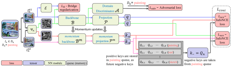
Figure 2: BrAD training architecture. $I_{n}^{a1},I_{n}^{a2}$ are random augmentations of an image $I_{n}\in D_{n}$. $\Psi_{n}(I_{n}^{a1}),\Psi_{n}(I_{n}^{a2})$ are their respective mappings to the bridge domain, $\Omega$, using a (learned) domain specific image-to-image mapping $\Psi_{n}$. The color of the arrows indicates the image that flows through the model: $I_{n}^{a1}$ (blue), $I_{n}^{a2}$ (pink), $\Psi_{n}(I_{n}^{a1})$ (green) and $\Psi_{n}(I_{n}^{a2})$ (red). The negative keys $k_{-}$ of the contrastive losses $L_{nce}$ come from a domain specific queue. We apply the $L_{\Omega}$ regularization, distilling from an edge-mapping $\mathcal{E}$ (can be even a simple Canny, see Sec. 4.4), forcing the bridge domain images to be similar to edge maps, which are (intuitively) less sensitive to domain shift. Finally, a domain discriminator $\mathcal{A}$ and an adversarial loss $\mathcal{L}_{adv}$ improve the domain invariance of the $\Omega$ projected images representations.

2 Related Work

Unsupervised Domain Adaptation (UDA). UDA [16] refers to transferring knowledge from a labeled source domain to an unlabeled target domain. Most UDA methods employ feature distribution alignment using: maximum discrepancy of domain distributions [48, 69, 35, 37, 52, 70, 25], adversarial domain classifier [14, 21, 36, 13, 55, 63, 50], and entropy optimization [46, 36, 26, 47]. GAN based image translation is used in [2, 21, 39, 49, 51, 29]. In [34, 58, 64] source domain data is replaced with a model pre-trained on the source. [38] uses low-level edge features to enforce consistency in UDA for monocular depth estimation. In Few-shot UDA (FUDA) [26, 65], only a few examples per class are labeled in the source domain, while the rest are unlabeled. In our work we take another step further and preform domain adaptation without seeing any labeled examples during training.

Domain Generalization (DG). DG addresses transferring knowledge to domains unseen during training. Most DG works perform supervised training on (a set of) labeled source domains. Methods for supervised DG include: distribution matching across domains [31, 33], adaptive weighting of different source domain losses [45], enforcing low rank of the latent representations [32] , and random source domains mixing [59]. Unsupervised DG (UDG) is a new task of training with unlabeled source domains introduced by [68]. The unlabeled source domains images are used for self-supervised pretraining followed by fitting a classifier to the learned representations via labeling a small portion of the source images. We show strong advantages of our method for the UDG setting, even when the unsupervised pretraining features are used directly via kNN without any further classifier fitting.

Self-Supervised Learning (SSL). SSL refers to learning strong semantic feature representations from unlabeled data. Historically, many pre-text tasks were proposed for SSL  [12, 41, 15, 67, 42, 27]. Recently, contrastive learning  [12, 61, 7, 8, 19, 9, 5, 17, 10, 6, 28, 54, 57, 66] has shown great promise and SOTA results. Contrastive methods usually optimize instance discrimination by making two augmentations of the same image closer in feature space than their distance to a set of negative anchors. In our experiments we show an advantage of our method over a direct application of popular SSL methods to multi-domain data, likely due to SSL methods tendency to separate domains before separating classes, avoided via the proposed use of a cross-domain bridge. Concurrently to our work, [60] successfully used HOG features for SSL in videos. Our approach can easily allow adoption of HOG or other hand-crafted edge-based features as an alternative regularization for the learned bridge domain, thus offering a general tool for further investigation of edges utility for contrastive SSL in future work.

Self-Supervised Learning for UDA and DG. Some UDA and DG methods employ SSL losses in their pipeline. SSL task of solving jigsaw puzzle was leveraged in [41] to aid UDA and DG.  [53] combine supervised learning on the source domain jointly with SSL on both domains. Recently [26, 65] proposed a cross-domain SSL approach for Few-shot UDA (FUDA), and [68] proposed an SSL method for UDG. As mentioned, we show strong advantages of our method for both FUDA and UDG tasks.

3 Method

Let ${\mathcal{D}=\{D_{n}}\}_{n=1}^{N}$ be a set of $N$ domains used for training (e.g., a pair of source and target domains in FUDA [26, 65], or a set of source domains in UDG [68]). Each domain $D_{n}$ is represented by a set of unlabeled images $\{I_{n}^{j}\}$, for clarity we will omit $j$ and denote by $I_{n}$ ‘an image’ from domain $D_{n}$. Our goal is to train a backbone model $\mathcal{B}$ (e.g., CNN) that projects any image $I_{n}\in D_{n}$ into a $d$-dimensional representation space $\mathcal{F}\subset\mathbb{R}^{d}$ (shared for all domains), in a way that for a class mapping $\mathcal{C}$ (unknown at training) and any $I_{n}\in D_{n}$ and $I_{m},I_{r}\in D_{m}$, s.t. $\mathcal{C}(I_{n})=\mathcal{C}(I_{m})\neq\mathcal{C}(I_{r})$: $||\mathcal{B}(I_{n})-\mathcal{B}(I_{m})||\ll||\mathcal{B}(I_{n})-\mathcal{B}(I_{r})||$ will likely be satisfied. Moreover, our overall goal is that this semantic alignment property will also generalize to other domains, even if they are not seen during training.

We train $\mathcal{B}$ using contrastive self-supervised learning extending the MocoV2 approach [9] to incorporate BrAD learning and other ideas explained below. Specifically, our training architecture (Figure 2) is comprised of the following components: (1) The backbone $\mathcal{B}:I\to\mathbb{R}^{d}$ (e.g., ResNet50 with GAP and $d=2048$) - it is the only thing kept after training, the rest of the components are used for training only and later discarded; (2) The projection head $\mathcal{P}:\mathbb{R}^{d}\to\mathbb{R}^{p}$ where $p<d$ (e.g., two-layer MLP with $p=128$) and with $\mathbb{L}_{2}$ normalization on top; (3) Separate negatives queue $\mathcal{Q}_{n}$ for each of the domains $D_{n}\in\mathcal{D}$ - as separating between domains is much easier than separating between classes, we observed that having a single queue (as in [9]) for all the domains hurts performance (as explained in Sec. 4.4); (4) A set of image-to-image models $\Psi_{n}:D_{n}\to\Omega$, for mapping each domain $D_{n}\in\mathcal{D}$ to the shared (across all seen and unseen domains) auxiliary BrAD domain $\Omega$ - the $\Psi_{n}$ are regularized to produce edge-like images which comprise $\Omega$, in Sec. 4 we explore and compare several options for $\Psi_{n}$; (5) Domain discriminator $\mathcal{A}:\mathbb{R}^{d}\to\{1,\cdots,N\}$, which is an adversarial domain classifier applied only to the $\Omega$ images representations, i.e., to $\mathcal{B}(\Psi_{n}(I_{n}))$, and trying to predict the original domain index $n$ of any image $I_{n}\in D_{n}$ projected to $\Omega$. Intuitively, learning to produce representations that confuse $\mathcal{A}$ better aligns the projections of all the different original domains inside $\Omega$. (6) The momentum models $\mathcal{B}^{m}$ and $\mathcal{P}^{m}$ (as in [9]): EMA-only updated copies of $\mathcal{B}$ and $\mathcal{P}$ respectively.

The training proceeds in batches of images randomly sampled from all the training domains $\mathcal{D}$ jointly. For clarity we will describe the training flow for a single input image $I_{n}\in D_{n}\in\mathcal{D}$. Having $I_{n}^{a1}$ and $I_{n}^{a2}$ be two augmentations of $I_{n}$, we first define the following contrastive loss:

$$\begin{split}\mathcal{L}_{cont}(I_{n})&=\mathcal{L}_{nce}(\mathcal{P}(\mathcal{B}(I_{n}^{a1})),\mathcal{P}^{m}(\mathcal{B}^{m}(\Psi_{n}(I_{n}^{a2}))),\mathcal{Q}_{n})\\ &+\mathcal{L}_{nce}(\mathcal{P}(\mathcal{B}(\Psi_{n}(I_{n}^{a1}))),\mathcal{P}^{m}(\mathcal{B}^{m}(I_{n}^{a2})),\mathcal{Q}_{n})\end{split}$$ (1)

where $\mathcal{L}_{nce}(q,k_{+},k_{-})$ is the standard InfoNCE loss [18, 19] with the query $q$, the positive key $k_{+}$ that attracts $q$, and the set of negative keys $k_{-}$ that repulse $q$. Our InfoNCE uses cosine similarity to compare queries and keys. Since in both $\mathcal{L}_{nce}$ summands of Eq. 1, the positive keys $k_{+}$ are always encoded via the momentum models $\mathcal{B}^{m}$ and $\mathcal{P}^{m}$ (not producing gradients), we need both these $\mathcal{L}_{nce}$ in order to train $\mathcal{B}$ and $\mathcal{P}$ to represent both the original training domains images $I_{n}\in D_{n}$ and their BrAD-mappings $\Psi_{n}(I_{n})\in\Omega$. Note that the first $\mathcal{L}_{nce}$ of Eq. 1 teaches $\mathcal{B}$ to extract $\Omega$-relevant features directly from each $D_{n}$, which means we can discard the BrAD-mapping models $\Psi_{n}$ after training and apply $\mathcal{B}$ even to unseen domains for which we do not have a learned BrAD-mapping. After each batch is processed, the batch images ‘momentum’ representations are (circularly) queued in accordance to their source domains:

$$\mathcal{Q}_{n}\leftarrow\mathcal{Q}_{n}\cup\{\mathcal{P}^{m}(\mathcal{B}^{m}(\Psi_{n}(I_{n}^{a2}))),\mathcal{P}^{m}(\mathcal{B}^{m}(I_{n}^{a2}))\}$$ (2)

Maintaining our queues in this way enables $D_{n}$ images from future training batches to contrast (in $\mathcal{F}$) not only against $\Omega$ projections of other $D_{n}$ images, but also against other images from $D_{n}$ - thus enabling our representation model $\mathcal{B}$ to complement its set of $\Omega$-specific features with some $D_{n}$-specific ones (e.g. color features). Additionally, we use the following adversarial loss:

$$\mathcal{L}_{adv}(I_{n})=CE(\mathcal{A}(\mathcal{B}(\Psi_{n}(I_{n}^{a1}))),n)$$ (3)

where $CE$ is the standard cross-entropy loss and $n\in\{1,\cdots,N\}$ is the correct domain index for the image $I_{n}$. We employ the standard (‘two-optimizers’ in PyTorch) adversarial training scheme for $\mathcal{L}_{adv}$. In each training batch, the domain discriminator $\mathcal{A}$ is minimizing $\mathcal{L}_{adv}$, while blocking $\mathcal{B}$ and $\Psi_{n}$ gradients, whereas $\mathcal{B}$ and $\Psi_{n}$ minimize the negative loss: $-\mathcal{L}_{adv}$, while blocking the $\mathcal{A}$ gradients. Note that we employ $\mathcal{L}_{adv}$ only for the $\Omega$ projections of the original domains, thus not requiring direct alignment between the domains of $\mathcal{D}$. Moreover, to reduce ‘competition’ between $\mathcal{L}_{adv}$ and $\mathcal{L}_{cont}$, we use the domain discriminator $\mathcal{A}$ directly on $\mathcal{B}$-generated representations (the final features) and not on the projection head $\mathcal{P}$-generated representations (temporary features used for efficiency in $\mathcal{L}_{cont}$). Lastly, we define the BrAD loss that regularizes the $\Psi_{n}$ models to produce edge-like images comprising the shared auxiliary BrAD domain $\Omega$, which we show to be very effective for different tasks in Sec. 4:

$$\mathcal{L}_{\Omega}(I_{n})=||\Psi_{n}(I_{n}^{a1})-\mathcal{E}(I_{n}^{a1})||^{2}$$ (4)

where $\mathcal{E}$ is some edge model, which could be heuristic, such as Canny edge detector [4], or pre-trained, such as HED [62], we explore and compare variants in Sec. 4.4. Finally, our full loss for image $I_{n}$ is therefore:

$$\mathcal{L}_{f}(I_{n})=\alpha_{1}\cdot\mathcal{L}_{cont}(I_{n})+\alpha_{2}\cdot\mathcal{L}_{\Omega}(I_{n})-\alpha_{3}\cdot\mathcal{L}_{adv}(I_{n})$$ (5)

where the sign in front of $\mathcal{L}_{adv}$ becomes positive when computing gradients for training the adversarial domain discriminator $\mathcal{A}$.

Implementation details. Our code is in PyTorch [11] and is based on the code of [9]. We set $\alpha_{1},\alpha_{2},\alpha_{3}=1$ in our experiments. The backbone $\mathcal{B}$ was ResNet-18 [20] for UDG experiments (same as in [68]), and ResNet-50 in FUDA and cross-benchmark generalization experiments (same as in [26]). We used batches of size $256$, SGD with momentum $0.9$, cosine LR-schedule (from LR 0.03 to 0.002) and trained for $250$ epochs for FUDA and $1000$ epochs for UDG (same as [68]). We set $|\mathcal{Q}_{n}|=min(64K,2\cdot|D_{n}|)$ and stored only a single pair of (momentum) representations generated from each domain image $I_{n}$ and its $\Omega$ projection (by $\Psi_{n}$). Furthermore, we found it slightly beneficial to exclude the cached version of $q$ from its $k_{-}$ negative keys set when computing the $\mathcal{L}_{nce}(q,k_{+},k_{-})$ losses. For $\mathcal{A}$ we used a $3$-layer MLP($1024,512,256$) with LeakyReLU, followed by a linear domain classifier. For the BrAD-mapping models $\Psi_{n}$ architecture, we used the architecture of HED [62] in its PyTorch implementation [40].

Source domains	{Paint. $\cup$ Real $\cup$ Sketch}			{Clipart $\cup$ Info. $\cup$ Quick.}
Target domain	Clipart	Info.	Quick.	Painting	Real	Sketch	Overall	Avg.
Label Fraction 1%
ERM	6.54	2.96	5.00	6.68	6.97	7.25	5.88	5.89
BYOL [17]	6.21	3.48	4.27	5.00	8.47	4.42	5.61	5.30
MoCo V2 [9, 19]	18.85	10.57	6.32	11.38	14.97	15.28	12.12	12.90
AdCo [22]	16.16	12.26	5.65	11.13	16.53	17.19	12.47	13.15
SimCLR V2 [8]	23.51	15.42	5.29	20.25	17.84	18.85	15.46	16.55
DIUL [68]	18.53	10.62	12.65	14.45	21.68	21.30	16.56	16.53
Ours (kNN)	40.65	14.00	21.28	16.80	22.29	25.72	22.35	23.46
Ours (linear cls.)	47.26	16.89	23.74	20.03	25.08	31.67	25.85	27.45
Label Fraction 5%
ERM	10.21	7.08	5.34	7.45	6.08	5.00	6.50	6.86
BYOL [17]	9.60	5.09	6.02	9.78	10.73	3.97	7.83	7.53
MoCo V2 [9, 19]	28.13	13.79	9.67	20.80	24.91	21.44	18.99	19.79
AdCo [22]	30.77	18.65	7.75	19.97	24.31	24.19	19.42	20.94
SimCLR V2 [8]	34.03	17.17	10.88	21.35	24.34	27.46	20.89	22.54
DIUL [68]	39.32	19.09	10.50	21.09	30.51	28.49	23.31	24.83
Ours (kNN)	55.75	18.15	26.93	24.29	33.33	37.54	31.12	32.66
Ours (linear cls.)	64.01	25.02	29.64	29.32	34.95	44.09	35.37	37.84
Label Fraction 10%
ERM	15.10	9.39	7.11	9.90	9.19	5.12	8.94	9.30
BYOL [17]	14.55	8.71	5.95	9.50	10.38	4.45	8.69	8.92
MoCo V2 [9, 19]	32.46	18.54	8.05	25.35	29.91	23.71	21.87	23.05
AdCo [22]	32.25	17.96	11.56	23.35	29.98	27.57	22.79	23.78
SimCLR V2 [8]	37.11	19.87	12.33	24.01	30.17	31.58	24.28	25.84
DIUL [68]	35.15	20.88	15.69	25.90	33.29	30.77	26.09	26.95
Ours (kNN)	60.78	19.76	31.56	26.06	37.43	41.38	34.77	36.16
Ours (linear cls.)	68.27	26.60	34.03	31.08	38.48	48.17	38.74	41.10

Table 1: Accuracy (%) results for UDG on DomainNet. All baseline results are taken from [68]. All methods use ResNet18 backbone and are unsupervisedly pretrained for 1000 epoches before training on the labeled (source only) data. All baselines use a linear classifier (for ours we also include a kNN result that does not utilize any supervised training). ERM indicates the randomly initialized ResNet18. Overall and Avg. indicate the overall test data accuracy and the mean of the per-domain accuracies, respectively. They are different since the test sets of different domains are not of the same size. The reported results are an average over $3$ runs. bold = best, blue = second best.

4 Results

As our BrAD approach is completely unsupervised during training, we used none or limited-supervision cross-domain tasks, specifically Unsupervised Domain Generalization (UDG) [68] and the Few-shot UDA (FUDA) [26, 65], for evaluating its performance and comparing to other self-supervised or source-labels-limited cross-domain methods. Additionally, we evaluate how BrAD and other self-supervised approaches generalize to unseen domains and unseen classes after being trained on a large-scale unlabeled cross-domain data, such as DomainNet [43].

Datasets. DomainNet [43] is the largest, most diverse and recent cross-domain benchmark to-date. It is comprised of $6$ domains: Real, Painting, Sketch, Clipart, Infograph and Quickdraw, with $345$ object classes, 48K - 173K images per domain, and average of $269$ images per class. PACS [30] is a standard domain generalization benchmark. It is comprised of $4$ domains: Photo, Art, Cartoon and Sketch, with $7$ object classes, 2.5K images per domain, and average of $357$ images per class. VisDA [44] is a simulation-to-real dataset with $12$ classes. The simulation domain is generated via repeated (80-480 times) 3D rendering of instances of 3D object models, 50-150 models per class. It is therefore comprised of only $\sim$1.5K distinct object instances. Office-Home [56] is a relatively small dataset consisting of $4$ domains: Art, Clipart, Product and Real, with $65$ classes, and an average of only $60$ images per class.

4.1 Unsupervised Domain Generalization

The UDG task is defined as: (i) unsupervised training on a set of source domains; (ii) using only a small labeled subset of source domain images to fit a linear classifier on top of the (frozen) features produced by the unsupervised model; and (iii) evaluating the resulting classifier performance on a set of target domains, unseen during training. In our UDG experiments we accurately followed the protocol of the UDG state-of-the-art (SOTA) method DIUL [68], including same backbone arch., same num. epochs, and same subset of classes used for training and testing. Same as [68], we evaluated on DomainNet [43] (Tab. 1) and PACS [30] (Tab. 2). In DomainNet, we train on Clipart, Infograph and Quickdraw and test on unseen Painting, Real and Sketch, and vice versa. For PACS we do a leave-one-domain-out test using the other three as source (repeating this for all domains). Unlike DIUL [68], who used additional full model fine-tuning when amount of source labels was $10\%$ of the source data size, our self-supervised model was never fine-tuned with the source labels (in all cases). Moreover, we also provide kNN results for our method, where we use our resulting features directly without any additional training.

As can be seen from Tab. 1 and Tab. 2, BrAD demonstrates significant gains (both in linear cls. and in kNN modes) not only over [68], but also over a variety of SOTA self-supervised pre-training baselines (probed with the classifier in exactly the same manner as [68] and as described above). This illustrates an important point, the BrAD idea seems to be effective in improving the generalization of self-supervised pre-training to unseen target domains, which, according to these results, seems quite difficult for the current self-supervised SOTA methods.

Target domain	Photo	Art.	Cartoon	Sketch	Avg.
Label Fraction 1%
ERM	10.90	11.21	14.33	18.83	13.82
BYOL [17]	11.20	14.53	16.21	10.01	12.99
MoCo V2 [9, 19]	22.97	15.58	23.65	25.27	21.87
AdCo [22]	26.13	17.11	22.96	23.37	22.39
SimCLR V2 [8]	30.94	17.43	30.16	25.20	25.93
DIUL [68]	27.78	19.82	27.51	29.54	26.16
Ours (kNN)	55.00	35.54	38.12	34.14	40.70
Ours (linear cls.)	61.81	33.57	43.47	36.37	43.81
Label Fraction 5%
ERM	14.15	18.67	13.37	18.34	16.13
BYOL [17]	26.55	17.79	21.87	19.65	21.47
MoCo V2 [9, 19]	37.39	25.57	28.11	31.16	30.56
AdCo [22]	37.65	28.21	28.52	30.35	31.18
SimCLR V2 [8]	54.67	35.92	35.31	36.84	40.68
DIUL [68]	44.61	39.25	36.41	36.53	39.20
Ours (kNN)	58.66	39.11	45.37	46.11	47.31
Ours (linear cls.)	65.22	41.35	50.88	50.68	52.03
Label Fraction 10%
ERM	16.27	16.62	18.40	12.01	15.82
BYOL [17]	27.01	25.94	20.98	19.69	23.40
MoCo V2 [9, 19]	44.19	25.85	33.53	24.97	32.14
AdCo [22]	46.51	30.21	31.45	22.96	32.78
SimCLR V2 [8]	54.65	37.65	46.00	28.25	41.64
DIUL [68]	53.37	39.91	46.41	30.17	42.47
Ours (kNN)	67.20	41.99	45.32	50.04	51.14
Ours (linear cls.)	72.17	44.20	50.01	55.66	55.51

Table 2: Accuracy (%) results for the UDG on PACS. For each target domain all other 3 are used as source domains for training. For other details about the number of runs, meaning of column titles and etc., please see Tab. 1 caption. All baseline results are taken from [68]. bold = best results, blue = second best.

4.2 Few-shot Unsupervised Domain Adaptation

We used the largest and most recent cross-domain dataset, DomainNet [43], to evaluate our BrAD approach FUDA [26, 65] performance. Same as in [65] (and as is common UDA practice), for this evaluation we used only $4$ domains: Clipart, Real, Painting and Sketch, and the source-target directions listed in Tab. 3. We follow the FUDA protocol defined in [65], where source domain has a single ($1$-shot) or three ($3$-shot) labeled images per-class and the rest of its images are provided as unlabeled. We used the same classes and the exact indices of the labeled samples for each case as provided by [65] for repeatability. Our results and comparison to other methods are summarized in Tab. 3. According to the protocol of [65], all compared methods models are initialized with ImageNet pre-training and operate in transductive setting. All the methods besides ours use the respective $1$ or $3$ samples per class during their training. In our case, we used those samples only during the inference - either as the search space in the kNN, or for training the linear classifier (on these few labeled source images only). All the methods besides ours are designed for working separately on each pair of source and target domains. Therefore, for the comparison to be comprehensive, we include results for our method in both our intended mode and a pairwise mode. In our intended mode (‘ours’ in Tab. 3) we train a single model on all the domains jointly. In the pairwise mode (‘ours pairwise’ in Tab. 3), we train $7$ separate models, one for each source-target domain pair. Besides showing a competitive advantage of our method in all modes, results in Tab. 3 indicate that multi-domain training has clear advantages in efficiency (single model vs. $7$ models), ease of use (no need to know the query domain), and performance (about $10\%$ better).

Source domain	Real	Real	Real	Painting	Painting	Clipart	Sketch
Target domain	Clipart	Painting	Sketch	Clipart	Real	Sketch	Painting	Avg.
Source-Only baseline [65]	18.4 / 30.2	30.6 / 44.2	16.7 / 25.7	16.2 / 24.6	28.9 / 49.8	12.7 / 24.2	10.5 / 23.2	19.1 / 31.7
MME[46]	13.8 / 22.8	29.2 / 46.5	9.7 / 14.5	16.0 / 25.1	26.0 / 50.0	13.4 / 20.1	14.4 / 24.9	17.5 / 29.1
CDAN [36]	16.0 / 30.0	25.7 / 40.1	12.9 / 21.7	12.6 / 21.4	19.5 / 40.8	7.20 / 17.1	8.00 / 19.7	14.6 / 27.3
MDDIA [23]	18.0 / 41.4	30.6 / 50.7	15.9 / 37.4	15.4 / 31.4	27.4 / 52.9	9.30 / 23.1	10.2 / 24.1	18.1 / 37.3
CAN [24]	18.3 / 28.1	22.1 / 33.5	16.7 / 25.0	13.2 / 24.7	23.9 / 46.9	11.1 / 23.3	12.1 / 20.1	16.8 / 28.8
CDS+SRDC+ENT [26]	23.1 / 36.6	40.0 / 54.0	22.2 / 35.5	24.1 / 38.1	35.1 / 57.6	18.8 / 35.4	25.2 / 45.1	26.9 / 43.2
CDS+MME+ENT [26]	35.4 / 47.4	36.7 / 52.8	33.4 / 43.2	25.6 / 41.2	29.4 / 56.4	19.3 / 37.5	22.5 / 41.1	28.9 / 45.6
PCS [65]	39.0 / 45.2	51.7 / 59.1	39.8 / 41.9	26.4 / 41.0	38.8 / 66.6	23.7 / 31.9	23.6 / 37.4	34.7 / 46.1
Ours pairwise (kNN)	43.6 / 49.5	50.4 / 57.0	41.7 / 47.9	35.9 / 41.0	44.2 / 60.7	34.5 / 42.4	36.1 / 45.5	40.9 / 49.1
Ours pairwise (linear cls.)	44.0 / 51.4	50.1 / 58.9	47.0 / 55.6	35.7 / 42.5	44.5 / 62.1	35.3 / 45.0	35.65 / 45.0	41.8 / 51.5
Ours (kNN)	46.4 / 57.6	52.0 / 59.4	50.5 / 58.9	45.1 / 55.3	49.3 / 61.3	48.3 / 56.4	49.0 / 59.3	48.6 / 58.3
Ours (linear cls.)	48.6 / 60.6	55.1 / 62.8	52.8 / 61.6	44.6 / 56.6	47.8 / 63.6	47.9 / 59.8	51.0 / 61.0	49.7 / 60.8

Table 3: 1-shot/3-shot accuracy (%) results for FUDA task [65] on DomianNet. All baseline results except CDS [26] are taken from [65]. The CDS results were kindly provided by its authors and are higher than those reported in [65]. bold = best results, blue = second best.

4.3 Generalization to unseen domains and classes

One of the interesting research questions to consider w.r.t. self-supervised learning - is how well it can generalize to unseen domains and classes. Assume one had access to a large collection of diverse unlabeled multi-domain data (e.g. unlabeled DomainNet [43]) needed for training a contrastive self-supervised model. However, also assume that the trained model would need to be used for inference in a few-shot scenario (i.e. with very little data) in a new unseen domain and for a new unseen set of classes. As an example, consider the situation we discussed in the introduction: our self-supervised system (pre-trained on some multi-domain data) would need to recognize in a real photo an instance of unseen before technical equipment after seeing it for the first time illustrated using some proprietary graphical style in some technical manual.

To test how leading self-supervised methods [9, 6, 5, 10, 66] deal with the proposed scenario (generalization to a mix of seen and unseen domains, as well as mostly unseen classes) and compare their performance to our approach, we conducted the following cross-dataset FUDA generalization experiment, whose results are provided in Tab. 4. We train all methods using their official codes and recommended hyper-parameter and backbone settings on the entire data of Clipart, Real, Painting and Sketch domains from DomainNet. Same ResNet50 backbone is used for all methods (including ours) except Dino [6] that uses the stronger ViT backbone for which it was optimized. We then evaluated the resulting models using a kNN classifier and the FUDA setting detailed in Sec. 4.2, on the OfficeHome [56], PACS [30], and VisDA [44] cross-domain datasets. In all cases, the $1$-shot and the $3$-shot source domain examples per class were sampled randomly and were kept the same for all methods. This experiment (sampling of shots) was repeated $5$ times and in Tab. 4 we report the averages. Similar to UDG experiments in Sec. 4.1, these results indicate again the difficulty for cross-domain generalization inherent to the popular self-supervised learning approaches, and the advantages of BrAD for improving this generalization. In Appendix C we provide many qualitative examples of cross-domain kNN results for the PACS datset, obtained using kNN in the features space of our self-supervised BrAD model trained on DomainNet.

Method	OfficeHome	PACS	VisDA
Dino [6]	12.41 / 16.97	30.90 / 34.67	25.02 / 28.14
SWAV[5]	13.26 / 17.80	31.14 / 33.09	25.65 / 29.26
SimSiam [10]	13.67 / 18.27	30.24 / 32.27	24.70 / 28.80
BarlowTwins[66]	17.86 / 24.06	41.18 / 46.18	25.34 / 30.47
MocoV2 [9]	17.64 / 22.63	49.00 / 54.25	30.34 / 36.10
Ours	21.79 / 28.21	55.61 / 63.00	32.98 / 40.22

Table 4: 1-shot / 3-shot accuracy (%) cross dataset results. The models are trained from scratch on DomainNet and tested on the OfficeHome, PACS and VisDA. We report an average over $5$ runs randomizing the shots. bold = best, blue = second best.

4.4 Ablation Studies

In Tab. 5 we evaluate the contribution of the different components of our approach using the FUDA task [26, 65] on the DomainNet dataset [43]. The experimental setting is described in Sec. 4.2 above. Specifically, we show how the average performance of the resulting model in $1$-shot / $3$-shots FUDA on DomainNet evolves starting from the vanilla MocoV2 [9] and adding: (i) DD: a domain discriminator ($\mathcal{A}$ in Eq. 3) - on its own it has a minor impact on performance ($\vbox{\hbox{\scalebox{1.0}{-}}}0.3/\vbox{\hbox{\scalebox{1.0}{+}}}0.1$); (ii) MQ: multiple negative queues ($\mathcal{Q}_{n}$) for contrastive loss - adds good boost to $1$-shot case ($\vbox{\hbox{\scalebox{1.0}{+}}}4.2/\vbox{\hbox{\scalebox{1.0}{+}}}0.4$) on its own, and strong boost for both modes when combined with DD ($\vbox{\hbox{\scalebox{1.0}{+}}}3.8/\vbox{\hbox{\scalebox{1.0}{+}}}6.0$); (iii) Canny BrAD: $\Psi_{n}$ in heuristic Canny [4] edge detector form - leads to a very strong performance boost ($\vbox{\hbox{\scalebox{1.0}{+}}}10.9/\vbox{\hbox{\scalebox{1.0}{+}}}11.9$) underlining the effectiveness of the BrAD idea; (iv) HED BrAD: $\Psi_{n}$ being a frozen HED [62] edge detector pre-trained on BSDS500 [1] dataset - we observe that even using a strong pre-trained edge detector model is not sufficient to further improve relative to the simpler Canny BrAD ($\vbox{\hbox{\scalebox{1.0}{-}}}1.7/\vbox{\hbox{\scalebox{1.0}{-}}}1.8$), this clearly highlights that BrAD models $\Psi_{n}$ need to be learned jointly (end-to-end) with the representation model $\mathcal{B}$ as we propose in our main approach; (v) learned BrAD: $\Psi_{n}$ being a HED [62] model trained end-to-end with the other components of our BrAD approach as described in Sec. 3 - underlining the need to learn the BrAD $\Psi_{n}$ models, this introduces a noticeable boost relative to the heuristic Canny BrAD ($\vbox{\hbox{\scalebox{1.0}{+}}}2.8/\vbox{\hbox{\scalebox{1.0}{+}}}2.3$) and overall compared to not using BrAD ($\vbox{\hbox{\scalebox{1.0}{+}}}13.7/\vbox{\hbox{\scalebox{1.0}{+}}}14.2$); (vi) Typical examples of comparison of edges generated by Canny, pretrained HED [62], and our learned BrAD are shown in Fig. 3 - as can be seen, both BrAD and HED discard the background noise, but unlike HED, BrAD learns to retain semantic details of shape and texture like house windows, giraffe spots, or person arm (additional examples are provided in Appendix A); (vii) Transductive / ImageNet pretrained: according to the FUDA experimental setting of PCS [65], used for all methods in our FUDA evaluation in Sec. 4.2, training starts from an ImageNet pretrained model and transductive paradigm is used for the unlabeled domains data - we have verified that the transductive setting consistently adds $\sim 4\%$ regardless of pretraining, while ImageNet pretraining has a more significant impact, adding $\sim 10\%$ to the performance.

		BrAD	Transd-	ImageNet
DD	MQ	$\Psi_{n}$	uctive	pretrained	1-shot	3-shots
-	-	-	-	-	16.8	21.9
✓	-	-	-	-	16.5	22.0
-	✓	-	-	-	21.0	22.3
✓	✓	-	-	-	20.6	27.9
✓	✓	Canny	-	-	31.5	39.8
✓	✓	HED	-	-	29.8	38.0
✓	✓	learned	-	-	34.3	42.1
✓	✓	learned	✓	-	37.8	47.1
✓	✓	learned	-	✓	44.1	55.2
✓	✓	learned	✓	✓	48.6	58.3
✓	✓	learned*	✓	✓	47.4	59.3
✓	✓	-	✓	✓	38.7	51.1
✓	✓	Canny	✓	✓	41.4	52.7
✓	✓	HED	✓	✓	41.6	51.9

Table 5: BrAD ablation study using the FUDA task on DomainNet dataset with knn classifier. bold = best, blue = second best. The highlighted row is our full method in Sec. 4.2 settings. The “learned*” is our full method without using HED pretrained weights.

Summarily adding all the above components and aligning to the experimental setting of PCS [65], we arrive at our main FUDA result (highlighted in Tab. 5). Moreover, we verified that our approach does not have a strong dependency on BSDS500 [1] dataset pre-training of the HED models [62] used as $\Psi_{n}$. Specifically, we randomly initialized the $\Psi_{n}$ BrAD models (that have HED architecture), and replaced the BSDS500 pretrained HED model used as $\mathcal{E}$ in the $\mathcal{L}_{\Omega}$ loss (Eq. 4) with a simple blurred Canny edge map (more details in the Supplementary). This way not having any BSDS500 pretrained weights anywhere in our system. As can be seen from the corresponding “learned*” row in Table 5, there is almost no change in the end result ($\vbox{\hbox{\scalebox{1.0}{-}}}1.2/\vbox{\hbox{\scalebox{1.0}{+}}}1.0$)) indicating our approach can work just as well without BSDS500 pretraining of HED. Please refer to Appendix B for more details. Finally, we verified that the strong gains we observed due to the introduction of BrAD models $\Psi_{n}$ do not disappear with ImageNet pretriaining and transductive setting. As can be seen in the corresponding rows of Tab. 5, both Canny and frozen HED BrAD variants maintain moderate gains of up to $2.9\%$ (over no-BrAD mode), while our full method with the learned $\Psi_{n}$ BrAD maintains large gains ($\vbox{\hbox{\scalebox{1.0}{+}}}9.9/\vbox{\hbox{\scalebox{1.0}{+}}}7.2$) as expected.

Real                  Art                    Sketch
Original  
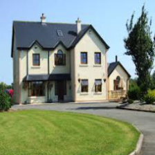
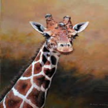
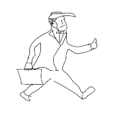
Canny [4]  
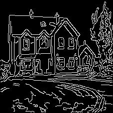
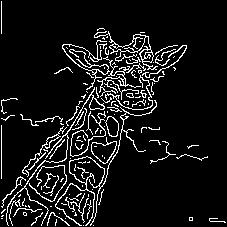
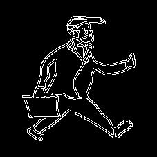
HED Zoom             HED[62]  
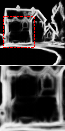
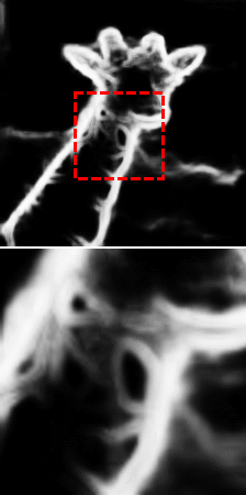
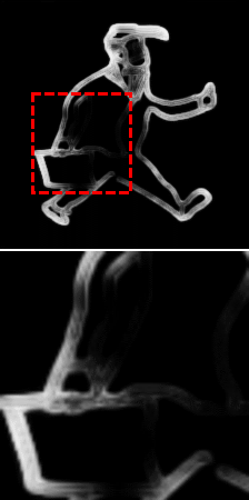
   BrAD Zoom                 BrAD  

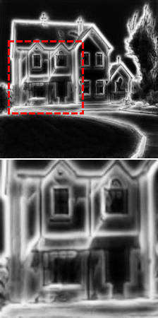
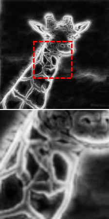
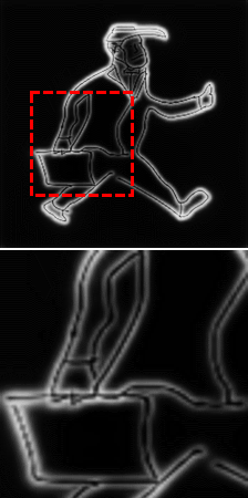
Figure 3: Edge images for different choices of $\Psi_{n}$: (i) Canny produces noisy images with many irrelevant edges; (ii) the HED mostly outlines the object and discards important internal texture; (iii) learned $\Psi_{n}$ keep the informative edges and the fine internal details while discarding most of the noise. More examples can be found in supplementary.

5 Conclusions and Limitations

In this paper, we have proposed a novel self-supervised cross-domain learning method based on semantically aligning (in feature space) all the domains to a common BrAD domain - a learned auxiliary bridge domain accompanied with relatively easy to learn image-to-image mappings to it. We have explored a special case of the edge-regularized BrAD - specifically driving BrAD to be a domain of edge-map-like images. In this implementation, we have shown significant advantages of our proposed approach for the important limited-source-labels tasks such as FUDA and UDG, as well as for a proposed task of generalization between cross-domain benchmarks to potentially unseen domains and classes. We observed a significant improvement over previous unsupervised and partially supervised methods for these tasks. Future work may also include exploration of the edge-like transforms used here as potentially useful augmentations for contrastive SSL in general.

Limitations of the current paper include: (i) intentional focusing only on edge-like bridge domains, which is one of the simplest BrAD one may construct. Naturally this bares limitations, e.g., lowering the relative importance of representing non-edge related features such as color. Thus, exploring other non-edge bridge domains is an important topic for future work; (ii) our current approach is built on top of a very useful, yet a single SSL method, namely, MoCo [9]. A direct extension could be employing our approach on top of a vision transformer backbone using the SSL method of [6], or more broadly, making it applicable to any SSL method; (iii) finally, our approach being completely unsupervised in pre-training, lacks control over which semantic classes are formed in the learned representation space, which is a common problem shared with most current SSL techniques that might lead to missing the classes that are under-represented in terms of different instance count in the unlabeled data. Addressing this in a follow-up work may include adding such control via some form of zero-shot or few-shot priming, or by training with coarse labels [3].

Acknowledgments

This material is based upon work supported by the Defense Advanced Research Projects Agency (DARPA) under Contract No. FA8750-19-C-1001. Any opinions, findings and conclusions or recommendations expressed in this material are those of the author(s) and do not necessarily reflect the views of DARPA. Raja Giryes was supported by ERC-StG grant no. 757497 (SPADE). Dina Katabi was supported by funding from the MIT-IBM Watson AI lab.

Appendix

Appendix A Additional edge map examples

Additional comparison of typical examples of BrAD variants generated by Canny [4], pretrained HED [62], and our ‘learned BrAD’ are shown in Figures 5 and 6. The images are taken from PACS dataset [30]. Figure 5 presents images from the domains Real and Art, while Figure 6 presents images from Sketch and Cartoon. As can be seen, both ‘learned BrAD’ and ‘HED BrAD’ variants discard the background noise, but unlike HED, ‘learned BrAD’ learns to retain semantic details of shape and texture. These retained details are intuitively highly useful for making the representations, learned using the ‘learned BrAD’ as the bridge domain $\Omega$, effective for the downstream tasks such as UDG or FUDA.

Appendix B BrAD loss $\mathcal{L}_{\Omega}$ without pretrained HED

When training BrAD domain mappings $\Psi_{n}$ we utilize the BrAD loss $\mathcal{L}_{\Omega}$ (Eq. (4) in the main paper, repeated in Eq. 6 below for convenience) for distilling from an edge-mapping $\mathcal{E}$ forcing the BrAD bridge domain $\Omega$ images to be similar to edge maps.

$$\mathcal{L}_{\Omega}(I_{n})=||\Psi_{n}(I_{n}^{a1})-\mathcal{E}(I_{n}^{a1})||_{2}^{2}$$ (6)

In the main variant of our approach the $\mathcal{E}$ is a HED [62] model pretrained on the BSDS500 dataset [1] and the $\Psi_{n}$ models are initialized with the same pretrained model. To avoid this use of BSDS500 as additional data, we tested alternative loss functions based on Canny [4] instead of HED [62], while randomly initializing $\Psi_{n}$. Since the edges in Canny edge-maps are only one pixel wide we apply a Gaussian blurring before comparing to the current $\Psi_{n}$ output. In our implementation we used a blur kernel of size $5$ with $\sigma=0.15$. We test both L1 and L2 norms, however, when using L1-norm we first stretch the $\Psi_{n}$ output to the range [0,1] for stability. Eq. 7 and Eq. 8 present both these variants of the Canny-based $\mathcal{L}_{\Omega}$ loss functions.

$$\mathcal{L}_{\Omega}(I_{n})=||\Psi_{n}(I_{n}^{a1})-Blur(\mathcal{E}_{Canny}(I_{n}^{a1}))||_{2}^{2}$$ (7)

$$\mathcal{L}_{\Omega}(I_{n})=||\mathcal{S}(\Psi_{n}(I_{n}^{a1}))-Blur(\mathcal{E}_{Canny}(I_{n}^{a1}))||_{1}$$ (8)

where $\mathcal{S}$ is a pixel-wise stretch function to the range [0,1]. Tab. 6 presents the average FUDA accuracy results on DomainNet using the above loss functions. As can be seen the differences in performance are quite small. Fig. 4 presents examples of BrAD images using the different losses. As can be clearly seen, all the learned BrAD variants (Fig. 4d-f) retain semantic details of shape and texture better than the fixed a-priori BrAD variants (Fig. 4b-c).

Loss	1-shot	3-shots
L2 Hed (equation 6)	48.64	58.31
L2 Canny (equation 7)	47.40	59.30
L1 Canny (equation 8)	47.77	58.66

Table 6: FUDA accuracy (%) results on DomainNet using different $L_{\Omega}$ BrAD losses. bold = best, blue = second best.

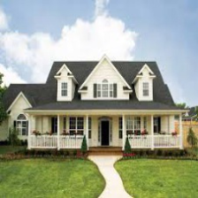
(a) Original image

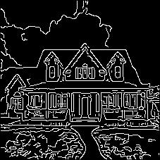
(b) Canny

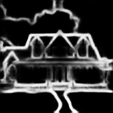
(c) Hed

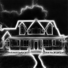
(d) L2 Hed-based $L_{\Omega}$ (Eq. 6)

(e) L2 Canny-based $L_{\Omega}$ (Eq. 7)

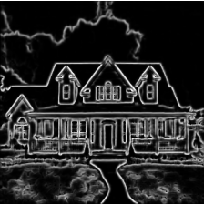
(f) L1 Canny-based $L_{\Omega}$ (Eq. 8)

Figure 4: Output images of BrAD mapping functions $\Psi_{n}$ trained using different loss functions $L_{\Omega}$ also compared to Canny [4] and HED [62] edge maps. Canny produces noisy images with many irrelevant edges, while HED mostly outlines the object and discards important internal texture. All learned $\Psi_{n}$ retain semantic details of shape and texture better than HED while discarding most of the noise. Please zoom.

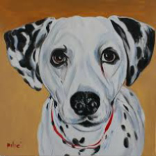
(a) Original

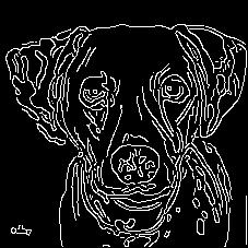
(b) Canny

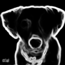
(c) HED

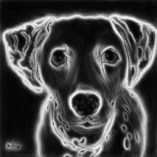
(d) Learned BrAD

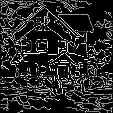
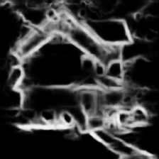
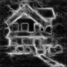
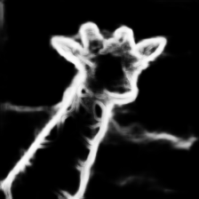
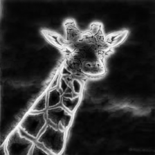
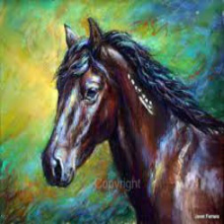
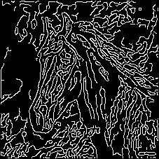
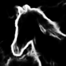
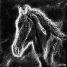
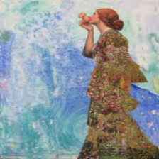
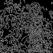
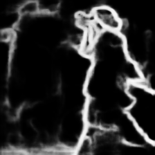
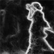
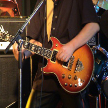
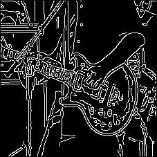
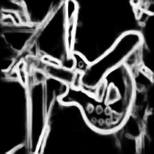
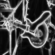
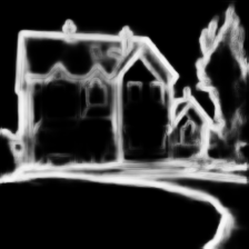
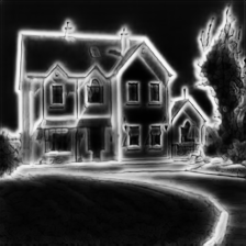
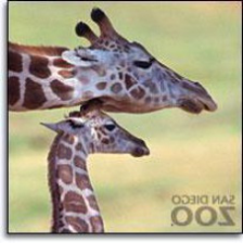
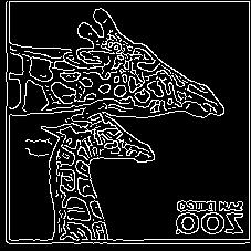
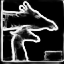
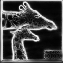
Figure 5: Edge images for different choices of $\Psi_{n}$. Images are taken from Real and Art domains of PACS dataset [30].

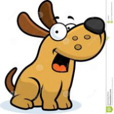
(a) Original

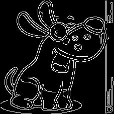
(b) Canny

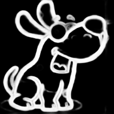
(c) HED

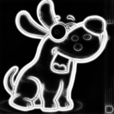
(d) Learned BrAD

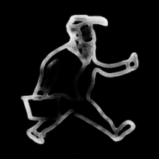
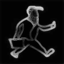
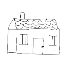
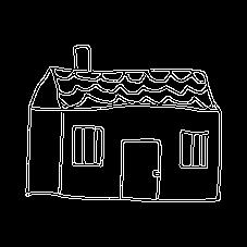
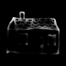
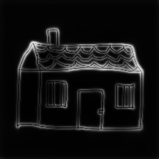
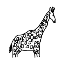
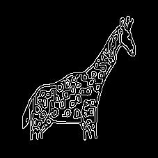
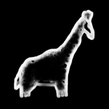
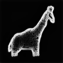
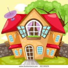
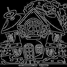
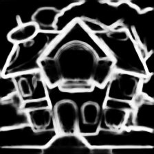
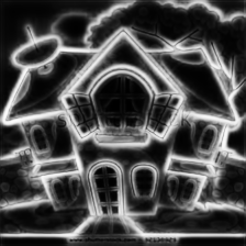
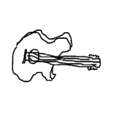
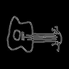
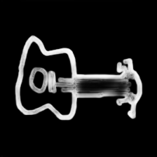
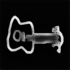
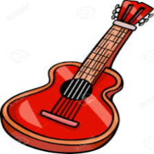
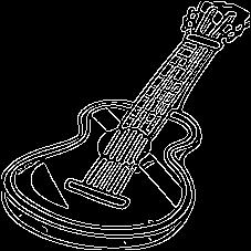
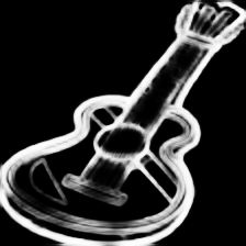
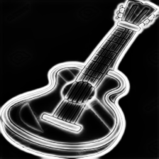
Figure 6: Edge images for different choices of $\Psi_{n}$. Images are taken from Cartoon and Sketch domains of PACS dataset [30].

Appendix C Demo

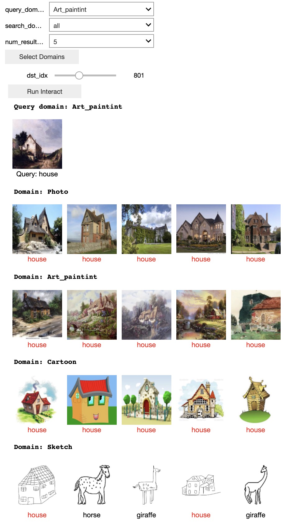
Figure 19: Random query example from our demo. For each query image (from PACS) we show the top $5$ image matches among the entire set of images in each of the $4$ PACS domains: Photo, Art/Painting, Cartoon, and Sketch. The matching is obtained using our self-supervised BrAD model trained using DomainNet data. The correct class is House. The text under each image is the ground truth class of that image in the PACS dataset.

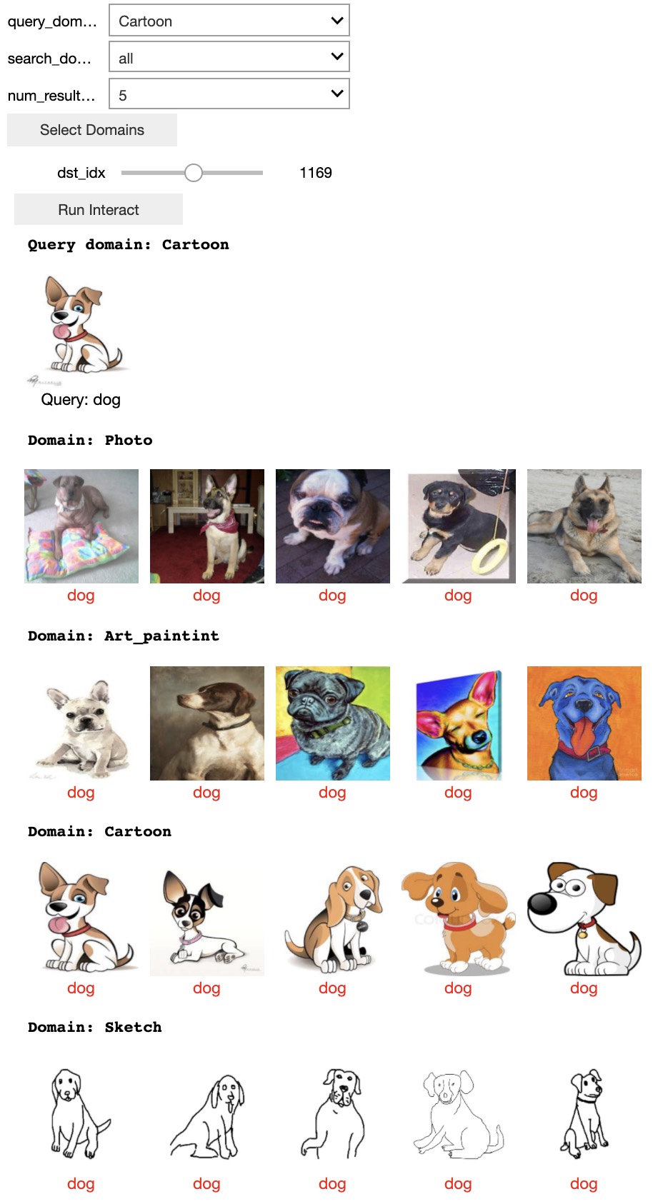
Figure 20: Random query example from our demo. For each query image (from PACS) we show the top $5$ image matches among the entire set of images in each of the $4$ PACS domains: Photo, Art/Painting, Cartoon, and Sketch. The matching is obtained using our self-supervised BrAD model trained using DomainNet data. The correct class is Dog. The text under each image is the ground truth class of that image in the PACS dataset.

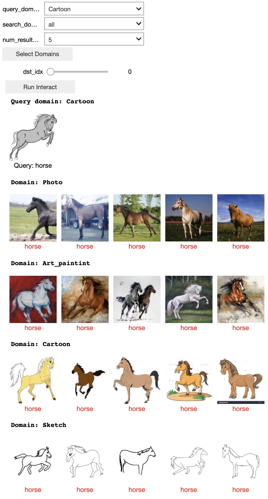
Figure 21: Random query example from our demo. For each query image (from PACS) we show the top $5$ image matches among the entire set of images in each of the $4$ PACS domains: Photo, Art/Painting, Cartoon, and Sketch. The matching is obtained using our self-supervised BrAD model trained using DomainNet data. The correct class is Horse. The text under each image is the ground truth class of that image in the PACS dataset.

In in Figs. 7, 8, 9, 10, 11, 12, 13, 14, 15, 16, 17, 18, 19, 20, 21 and 22 we showcase the domain alignment capabilities of the feature representation learned without supervision using our BrAD approach. Each example shows top-$5$ nearest neighbors of a random query image (from the PACS dataset) searched in the entire set of images of each of the $4$ different PACS domains: Photo, Art/Painting, Cartoon, and Sketch. All images are encoded using our self-supervised BrAD model trained on DomainNet dataset.

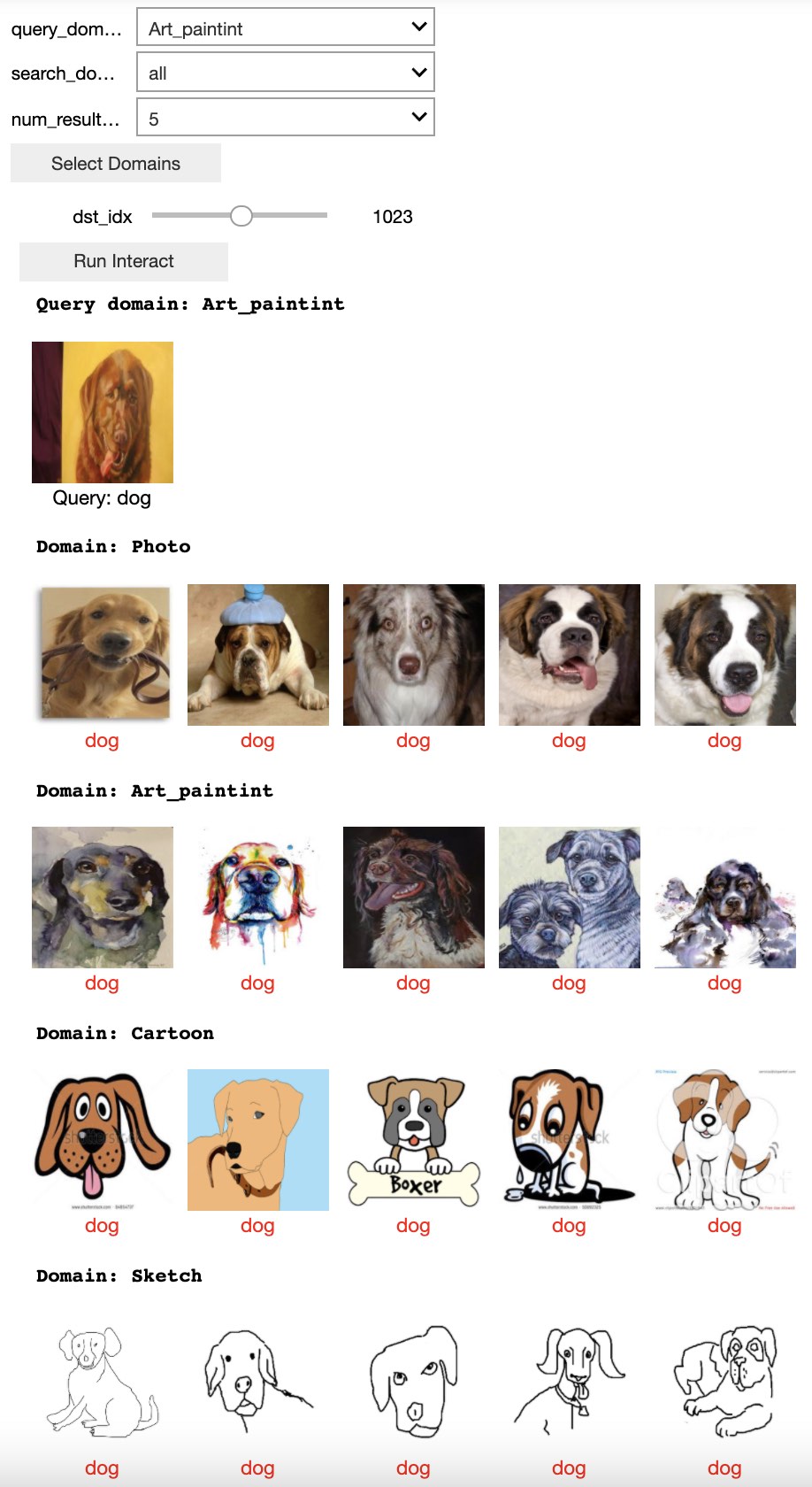
Figure 7: Random query example from our demo. For each query image (from PACS) we show the top $5$ image matches among the entire set of images in each of the $4$ PACS domains: Photo, Art/Painting, Cartoon, and Sketch. The matching is obtained using our self-supervised BrAD model trained using DomainNet data. The correct class is Dog. The text under each image is the ground truth class of that image in the PACS dataset.

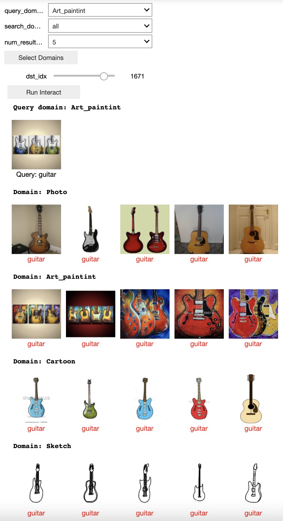
Figure 8: Random query example from our demo. For each query image (from PACS) we show the top $5$ image matches among the entire set of images in each of the $4$ PACS domains: Photo, Art/Painting, Cartoon, and Sketch. The matching is obtained using our self-supervised BrAD model trained using DomainNet data. The correct class is Guitar. The text under each image is the ground truth class of that image in the PACS dataset.

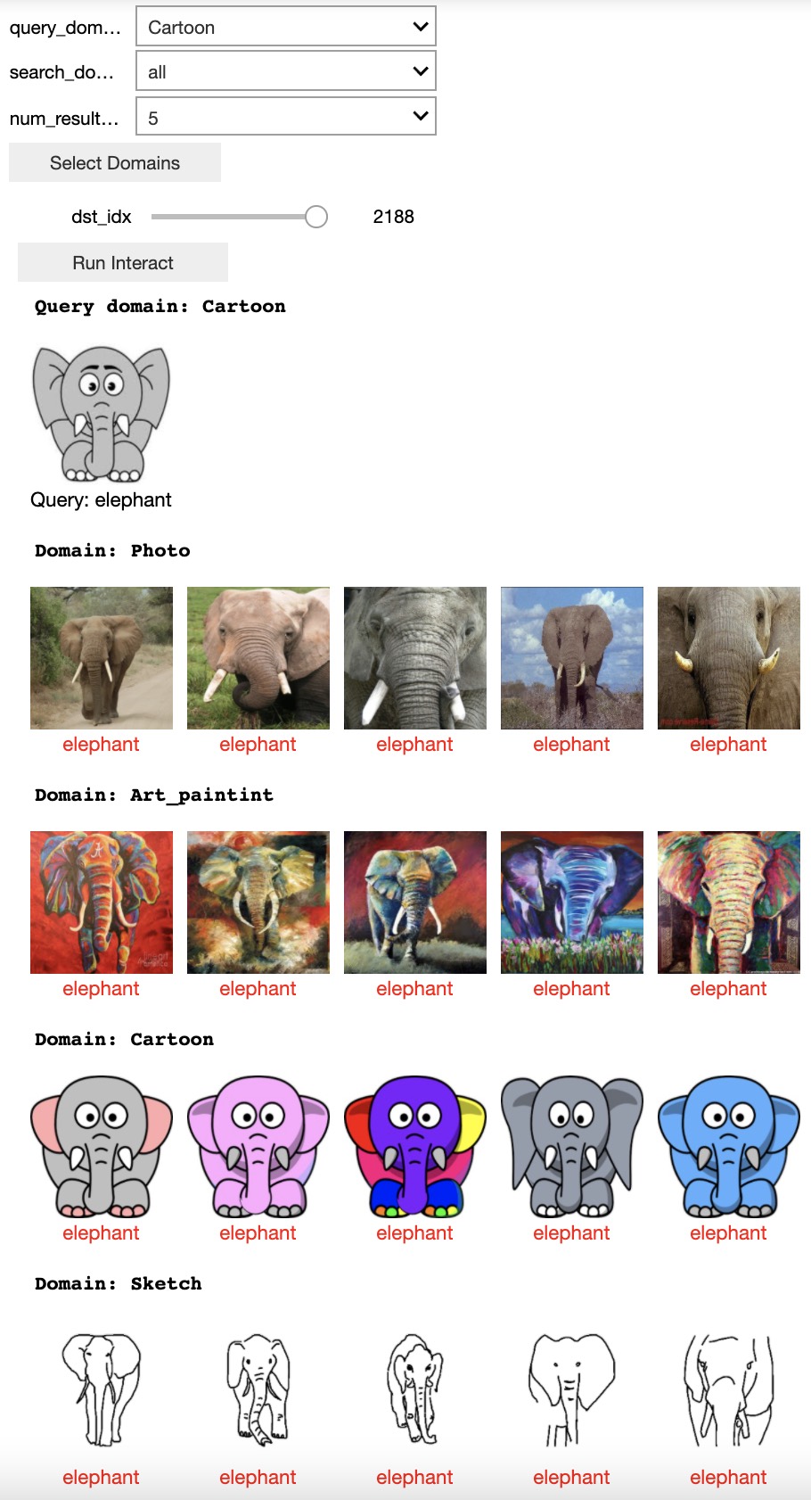
Figure 9: Random query example from our demo. For each query image (from PACS) we show the top $5$ image matches among the entire set of images in each of the $4$ PACS domains: Photo, Art/Painting, Cartoon, and Sketch. The matching is obtained using our self-supervised BrAD model trained using DomainNet data. The correct class is Elephant. The text under each image is the ground truth class of that image in the PACS dataset.

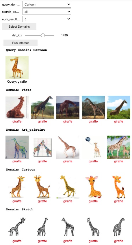
Figure 10: Random query example from our demo. For each query image (from PACS) we show the top $5$ image matches among the entire set of images in each of the $4$ PACS domains: Photo, Art/Painting, Cartoon, and Sketch. The matching is obtained using our self-supervised BrAD model trained using DomainNet data. The correct class is Giraffe. The text under each image is the ground truth class of that image in the PACS dataset.

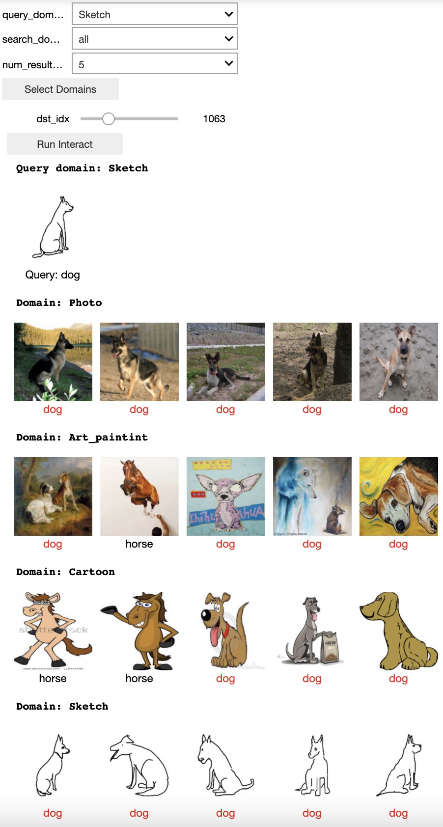
Figure 11: Random query example from our demo. For each query image (from PACS) we show the top $5$ image matches among the entire set of images in each of the $4$ PACS domains: Photo, Art/Painting, Cartoon, and Sketch. The matching is obtained using our self-supervised BrAD model trained using DomainNet data. The correct class is Dog. The text under each image is the ground truth class of that image in the PACS dataset.

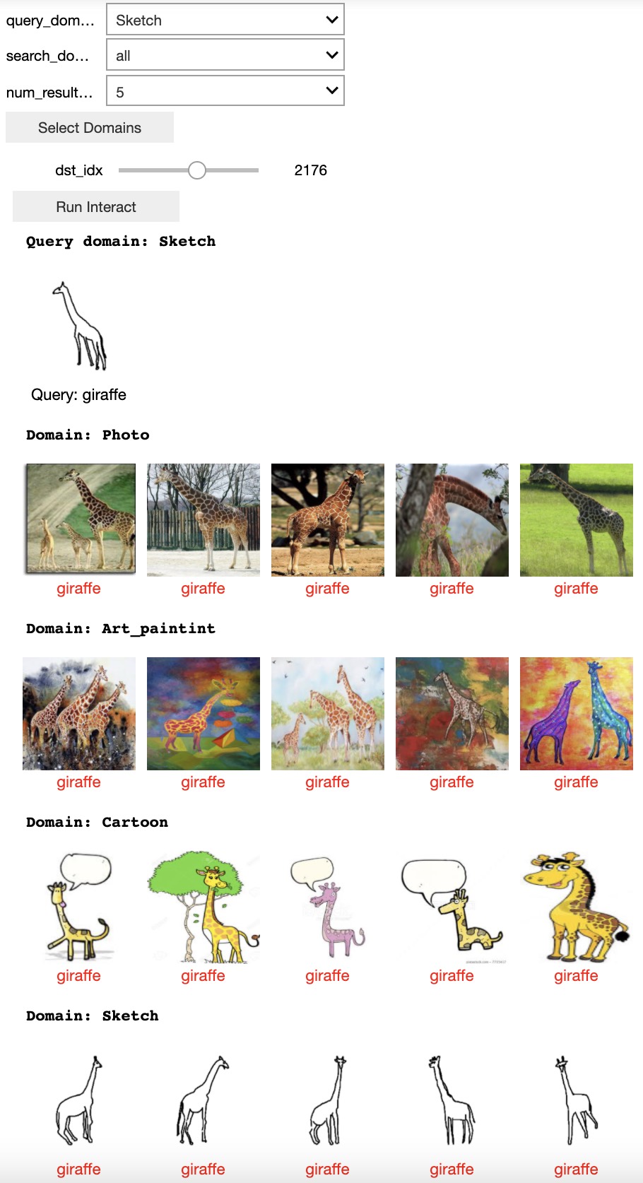
Figure 12: Random query example from our demo. For each query image (from PACS) we show the top $5$ image matches among the entire set of images in each of the $4$ PACS domains: Photo, Art/Painting, Cartoon, and Sketch. The matching is obtained using our self-supervised BrAD model trained using DomainNet data. The correct class is Giraffe. The text under each image is the ground truth class of that image in the PACS dataset.

Figure 13: Random query example from our demo. For each query image (from PACS) we show the top $5$ image matches among the entire set of images in each of the $4$ PACS domains: Photo, Art/Painting, Cartoon, and Sketch. The matching is obtained using our self-supervised BrAD model trained using DomainNet data. The correct class is House. The text under each image is the ground truth class of that image in the PACS dataset.

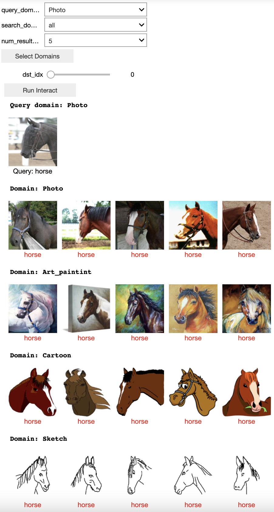
Figure 14: Random query example from our demo. For each query image (from PACS) we show the top $5$ image matches among the entire set of images in each of the $4$ PACS domains: Photo, Art/Painting, Cartoon, and Sketch. The matching is obtained using our self-supervised BrAD model trained using DomainNet data. The correct class is Horse. The text under each image is the ground truth class of that image in the PACS dataset.

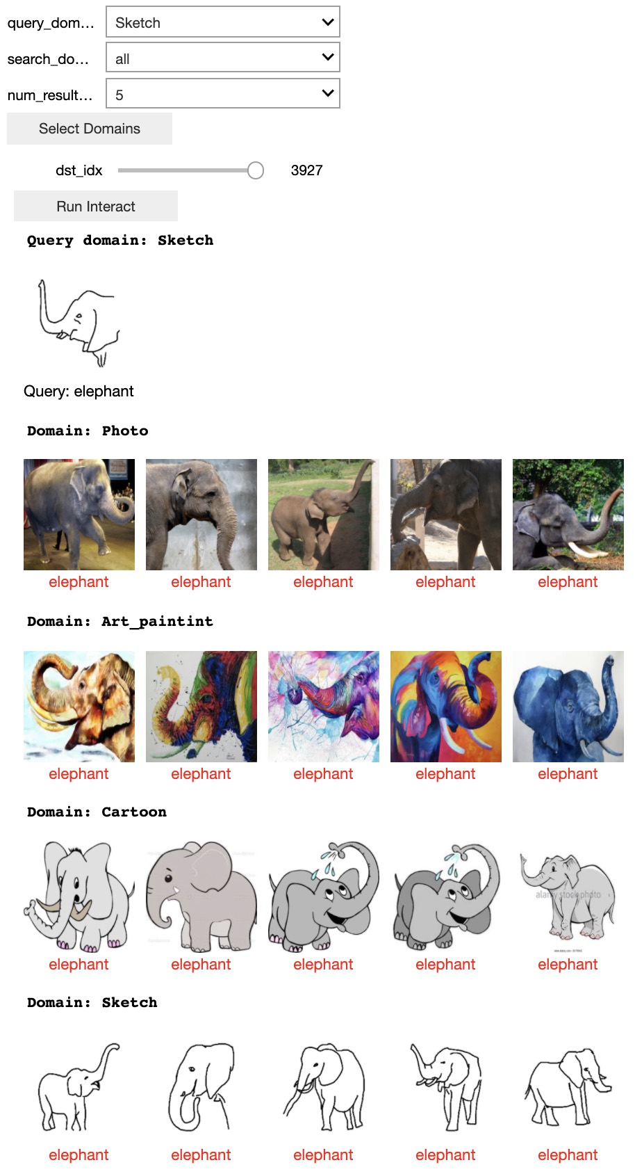
Figure 15: Random query example from our demo. For each query image (from PACS) we show the top $5$ image matches among the entire set of images in each of the $4$ PACS domains: Photo, Art/Painting, Cartoon, and Sketch. The matching is obtained using our self-supervised BrAD model trained using DomainNet data. The correct class is Elephant. The text under each image is the ground truth class of that image in the PACS dataset.

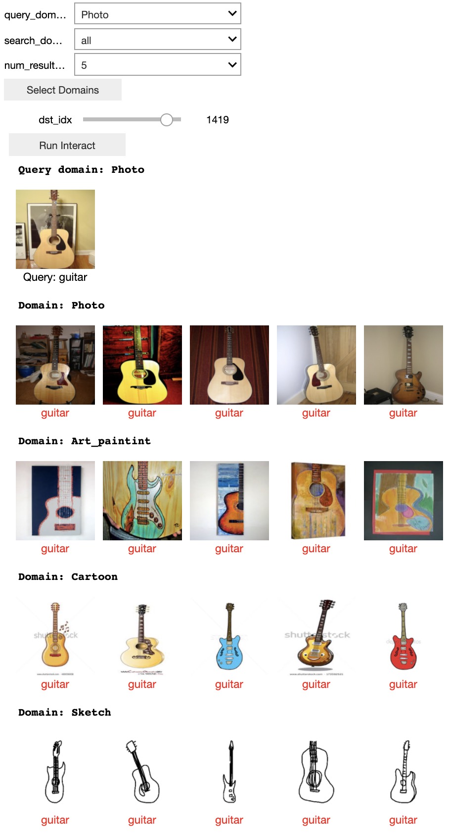
Figure 16: Random query example from our demo. For each query image (from PACS) we show the top $5$ image matches among the entire set of images in each of the $4$ PACS domains: Photo, Art/Painting, Cartoon, and Sketch. The matching is obtained using our self-supervised BrAD model trained using DomainNet data. The correct class is Guitar. The text under each image is the ground truth class of that image in the PACS dataset.

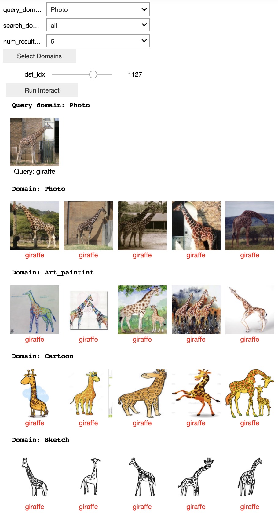
Figure 17: Random query example from our demo. For each query image (from PACS) we show the top $5$ image matches among the entire set of images in each of the $4$ PACS domains: Photo, Art/Painting, Cartoon, and Sketch. The matching is obtained using our self-supervised BrAD model trained using DomainNet data. The correct class is Giraffe. The text under each image is the ground truth class of that image in the PACS dataset.

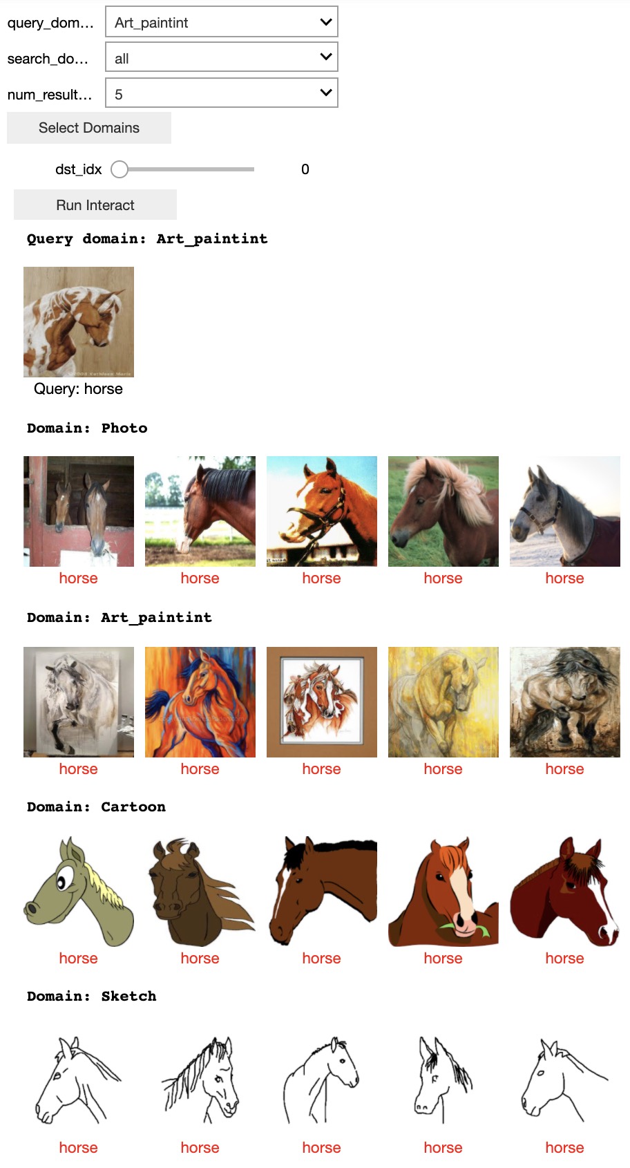
Figure 18: Random query example from our demo. For each query image (from PACS) we show the top $5$ image matches among the entire set of images in each of the $4$ PACS domains: Photo, Art/Painting, Cartoon, and Sketch. The matching is obtained using our self-supervised BrAD model trained using DomainNet data. The correct class is Horse. The text under each image is the ground truth class of that image in the PACS dataset.

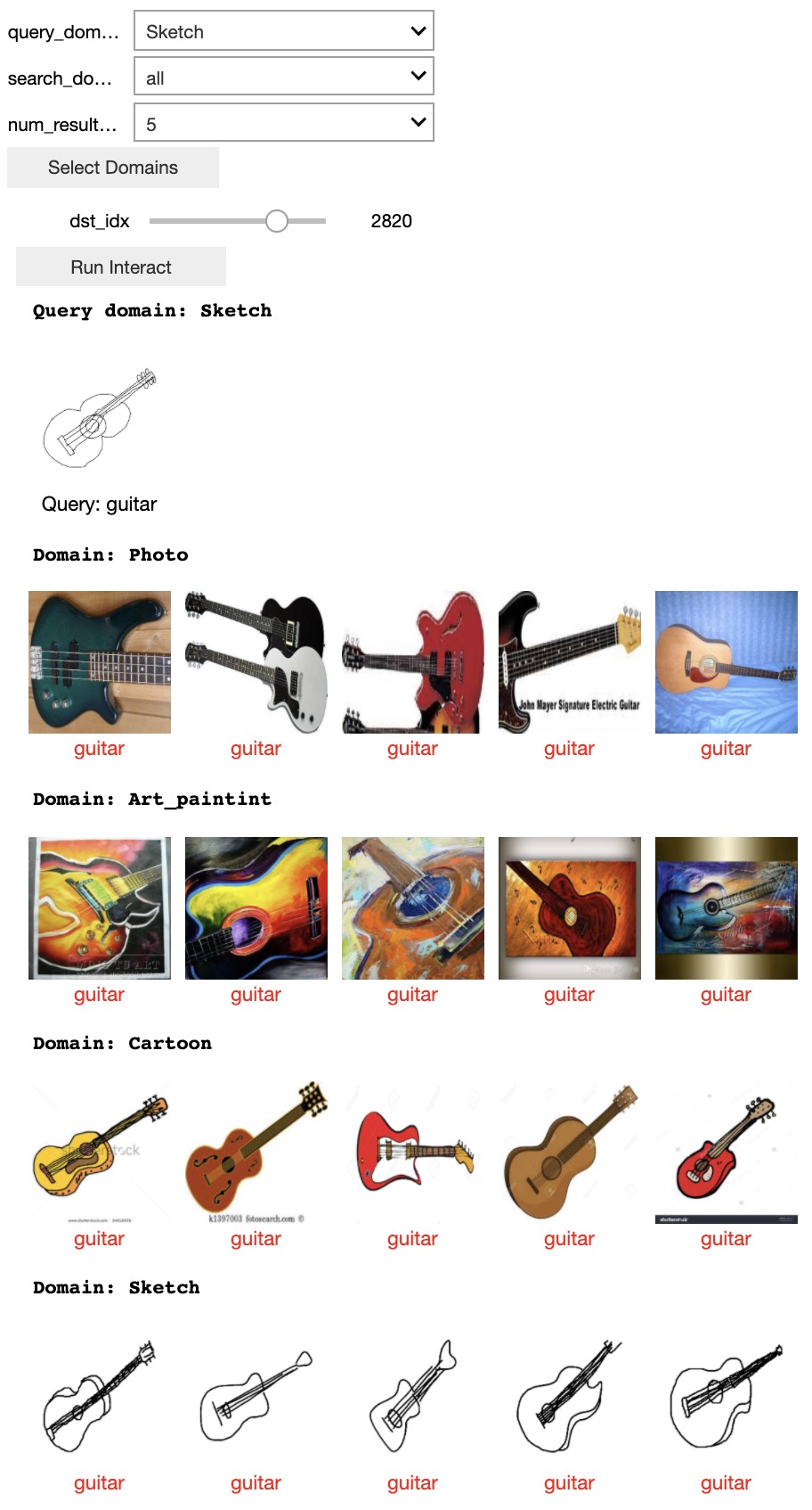
Figure 22: Random query example from our demo. For each query image (from PACS) we show the top $5$ image matches among the entire set of images in each of the $4$ PACS domains: Photo, Art/Painting, Cartoon, and Sketch. The matching is obtained using our self-supervised BrAD model trained using DomainNet data. The correct class is Guitar. The text under each image is the ground truth class of that image in the PACS dataset.

References

- [1] Pablo Arbelaez, Michael Maire, Charless Fowlkes, and Jitendra Malik. Contour detection and hierarchical image segmentation. IEEE Trans. Pattern Anal. Mach. Intell., 33(5):898–916, May 2011.
- [2] Konstantinos Bousmalis, Nathan Silberman, David Dohan, Dumitru Erhan, and Dilip Krishnan. Unsupervised pixel-level domain adaptation with generative adversarial networks. In Proceedings of the IEEE Conference on Computer Vision and Pattern Recognition (CVPR), July 2017.
- [3] Guy Bukchin, Eli Schwartz, Kate Saenko, Ori Shahar, Rogerio Feris, Raja Giryes, and Leonid Karlinsky. Fine-grained angular contrastive learning with coarse labels. In Proceedings of the IEEE/CVF Conference on Computer Vision and Pattern Recognition (CVPR), pages 8730–8740, June 2021.
- [4] John Canny. A computational approach to edge detection. IEEE Transactions on pattern analysis and machine intelligence, (6):679–698, 1986.
- [5] Mathilde Caron, Ishan Misra, Julien Mairal, Priya Goyal, Piotr Bojanowski, and Armand Joulin. Unsupervised learning of visual features by contrasting cluster assignments. In Advances in Neural Information Processing Systems (NeurIPS), 2020.
- [6] Mathilde Caron, Hugo Touvron, Ishan Misra, Hervé Jégou, Julien Mairal, Piotr Bojanowski, and Armand Joulin. Emerging properties in self-supervised vision transformers. In Proceedings of the International Conference on Computer Vision (ICCV), 2021.
- [7] Ting Chen, Simon Kornblith, Mohammad Norouzi, and Geoffrey E. Hinton. A simple framework for contrastive learning of visual representations. In International Conference on Machine Learning, (ICML), 2020.
- [8] Ting Chen, Simon Kornblith, Kevin Swersky, Mohammad Norouzi, and Geoffrey E Hinton. Big self-supervised models are strong semi-supervised learners. In Advances in Neural Information Processing Systems (NeurIPS), 2020.
- [9] Xinlei Chen, Haoqi Fan, Ross Girshick, and Kaiming He. Improved baselines with momentum contrastive learning. arXiv preprint arXiv:2003.04297, 2020.
- [10] Xinlei Chen and Kaiming He. Exploring simple siamese representation learning. In Proceedings of the IEEE/CVF Conference on Computer Vision and Pattern Recognition (CVPR), pages 15750–15758, 2021.
- [11] R. Collobert, K. Kavukcuoglu, and C. Farabet. Torch7: A matlab-like environment for machine learning. In BigLearn, NIPS Workshop, 2011.
- [12] Alexey Dosovitskiy, Jost Tobias Springenberg, Martin Riedmiller, and Thomas Brox. Discriminative unsupervised feature learning with convolutional neural networks. In Advances in neural information processing systems (NIPS), pages 766–774, 2014.
- [13] Yaroslav Ganin and Victor Lempitsky. Unsupervised domain adaptation by backpropagation. In International conference on Machine Learning (ICML), pages 1180–1189. PMLR, 2015.
- [14] Yaroslav Ganin, Evgeniya Ustinova, Hana Ajakan, Pascal Germain, Hugo Larochelle, François Laviolette, Mario Marchand, and Victor Lempitsky. Domain-adversarial training of neural networks. The journal of machine learning research, 17(1):2096–2030, 2016.
- [15] Spyros Gidaris, Praveer Singh, and Nikos Komodakis. Unsupervised representation learning by predicting image rotations. In International Conference on Learning Representations, (ICLR), 2018.
- [16] Raghuraman Gopalan, Ruonan Li, and Rama Chellappa. Domain adaptation for object recognition: An unsupervised approach. In International Conference on Computer Vision (ICCV), pages 999–1006. IEEE, 2011.
- [17] Jean-Bastien Grill, Florian Strub, Florent Altché, Corentin Tallec, Pierre Richemond, Elena Buchatskaya, Carl Doersch, Bernardo Avila Pires, Zhaohan Guo, Mohammad Gheshlaghi Azar, Bilal Piot, koray kavukcuoglu, Remi Munos, and Michal Valko. Bootstrap your own latent - a new approach to self-supervised learning. In Advances in Neural Information Processing Systems (NeurIPS), 2020.
- [18] Michael Gutmann and Aapo Hyvärinen. Noise-contrastive estimation: A new estimation principle for unnormalized statistical models. In Proceedings of the Thirteenth International Conference on Artificial Intelligence and Statistics, pages 297–304, 2010.
- [19] Kaiming He, Haoqi Fan, Yuxin Wu, Saining Xie, and Ross Girshick. Momentum contrast for unsupervised visual representation learning. In Proceedings of the IEEE/CVF Conference on Computer Vision and Pattern Recognition (CVPR), pages 9729–9738, 2020.
- [20] Kaiming He, Xiangyu Zhang, Shaoqing Ren, and Jian Sun. Deep residual learning for image recognition. In Proceedings of the IEEE Conference on Computer Vision and Pattern Recognition (CVPR), June 2016.
- [21] Judy Hoffman, Eric Tzeng, Taesung Park, Jun-Yan Zhu, Phillip Isola, Kate Saenko, Alexei Efros, and Trevor Darrell. Cycada: Cycle-consistent adversarial domain adaptation. In International conference on machine learning (ICML), pages 1989–1998. PMLR, 2018.
- [22] Qianjiang Hu, Xiao Wang, Wei Hu, and Guo-Jun Qi. Adco: Adversarial contrast for efficient learning of unsupervised representations from self-trained negative adversaries. In Proceedings of the IEEE/CVF Conference on Computer Vision and Pattern Recognition, pages 1074–1083, 2021.
- [23] X. Jiang, Q. Lao, S. Matwin, and M. Havaei. Implicit class-conditioned domain alignment for unsupervised domain adaptation. 2020.
- [24] G. Kang, L. Jiang, Y. Yang, and A. G. Hauptmann. Contrastive adaptation network for unsupervised domain adaptation. In Proceedings of the IEEE Conference on Computer Vision and Pattern Recognition (CVPR), pages 4893–4902, 2019.
- [25] Qi Kang, Siya Yao, MengChu Zhou, Kai Zhang, and Abdullah Abusorrah. Enhanced subspace distribution matching for fast visual domain adaptation. IEEE Transactions on Computational Social Systems, 7(4):1047–1057, 2020.
- [26] Donghyun Kim, Kuniaki Saito, Tae-Hyun Oh, Bryan A Plummer, Stan Sclaroff, and Kate Saenko. Cds: Cross-domain self-supervised pre-training. In Proceedings of the IEEE/CVF International Conference on Computer Vision (ICCV), pages 9123–9132, 2021.
- [27] Soroush Abbasi Koohpayegani, Ajinkya Tejankar, and Hamed Pirsiavash. Mean shift for self-supervised learning. arXiv preprint arXiv:2105.07269, 2021.
- [28] Klemen Kotar, Gabriel Ilharco, Ludwig Schmidt, Kiana Ehsani, and Roozbeh Mottaghi. Contrasting contrastive self-supervised representation learning pipelines. In Proceedings of the IEEE/CVF International Conference on Computer Vision, pages 9949–9959, 2021.
- [29] Seunghun Lee, Sunghyun Cho, and Sunghoon Im. Dranet: Disentangling representation and adaptation networks for unsupervised cross-domain adaptation. In Proceedings of the IEEE/CVF Conference on Computer Vision and Pattern Recognition (CVPR), pages 15252–15261, June 2021.
- [30] Da Li, Yongxin Yang, Yi-Zhe Song, and Timothy M. Hospedales. Deeper, broader and artier domain generalization. In Proceedings of the IEEE International Conference on Computer Vision (ICCV), Oct 2017.
- [31] Haoliang Li, Sinno Jialin Pan, Shiqi Wang, and Alex C Kot. Domain generalization with adversarial feature learning. In Proceedings of the IEEE Conference on Computer Vision and Pattern Recognition, pages 5400–5409, 2018.
- [32] Haoliang Li, YuFei Wang, Renjie Wan, Shiqi Wang, Tie-Qiang Li, and Alex C Kot. Domain generalization for medical imaging classification with linear-dependency regularization. NeurIPS, 2020.
- [33] Ya Li, Xinmei Tian, Mingming Gong, Yajing Liu, Tongliang Liu, Kun Zhang, and Dacheng Tao. Deep domain generalization via conditional invariant adversarial networks. In Proceedings of the European Conference on Computer Vision (ECCV), pages 624–639, 2018.
- [34] Jian Liang, Dapeng Hu, and Jiashi Feng. Do we really need to access the source data? source hypothesis transfer for unsupervised domain adaptation. In International Conference on Machine Learning (ICML), pages 6028–6039. PMLR, 2020.
- [35] Mingsheng Long, Yue Cao, Jianmin Wang, and Michael Jordan. Learning transferable features with deep adaptation networks. In International Conference on Machine Learning (ICML), pages 97–105. PMLR, 2015.
- [36] M. Long, Z. Cao, J. Wang, and M. Jordan. Conditional adversarial domain adaptation. Advances in Neural Information Processing Systems, pages 1640–1650, 2018.
- [37] Mingsheng Long, Han Zhu, Jianmin Wang, and Michael I Jordan. Unsupervised domain adaptation with residual transfer networks. In Proceedings of the 30th International Conference on Neural Information Processing Systems (NIPS), pages 136–144, 2016.
- [38] Adrian Lopez-Rodriguez and Krystian Mikolajczyk. Desc: Domain adaptation for depth estimation via semantic consistency. arXiv preprint arXiv:2009.01579, 2020.
- [39] Zak Murez, Soheil Kolouri, David Kriegman, Ravi Ramamoorthi, and Kyungnam Kim. Image to image translation for domain adaptation. In Proceedings of the IEEE Conference on Computer Vision and Pattern Recognition (CVPR), June 2018.
- [40] Simon Niklaus. A reimplementation of HED using PyTorch. https://github.com/sniklaus/pytorch-hed, 2018.
- [41] Mehdi Noroozi and Paolo Favaro. Unsupervised learning of visual representations by solving jigsaw puzzles. In European Conference on Computer Vision (ECCV), pages 69–84. Springer, 2016.
- [42] Deepak Pathak, Philipp Krahenbuhl, Jeff Donahue, Trevor Darrell, and Alexei A Efros. Context encoders: Feature learning by inpainting. In Proceedings of the IEEE conference on computer vision and pattern recognition (CVPR), pages 2536–2544, 2016.
- [43] Xingchao Peng, Qinxun Bai, Xide Xia, Zijun Huang, Kate Saenko, and Bo Wang. Moment matching for multi-source domain adaptation. In Proceedings of the IEEE International Conference on Computer Vision (ICCV), pages 1406–1415, 2019.
- [44] Xingchao Peng, Ben Usman, Neela Kaushik, Judy Hoffman, Dequan Wang, and Kate Saenko. Visda: The visual domain adaptation challenge, 2017.
- [45] Shiori Sagawa, Pang Wei Koh, Tatsunori B Hashimoto, and Percy Liang. Distributionally robust neural networks for group shifts: On the importance of regularization for worst-case generalization. arXiv preprint arXiv:1911.08731, 2019.
- [46] K. Saito, D. Kim, S. Sclaroff, T. Darrell, and K. Saenk. Semi-supervised domain adaptation via minimax entropy. In Proceedings of the IEEE International Conference on Computer Vision (ICCV), pages 8050–8058, 2019.
- [47] Kuniaki Saito, Donghyun Kim, Stan Sclaroff, and Kate Saenko. Universal domain adaptation through self supervision. Advances in Neural Information Processing Systems, 33, 2020.
- [48] Kuniaki Saito, Kohei Watanabe, Yoshitaka Ushiku, and Tatsuya Harada. Maximum classifier discrepancy for unsupervised domain adaptation. In Proceedings of the IEEE Conference on Computer Vision and Pattern Recognition (CVPR), June 2018.
- [49] Swami Sankaranarayanan, Yogesh Balaji, Carlos D. Castillo, and Rama Chellappa. Generate to adapt: Aligning domains using generative adversarial networks. In Proceedings of the IEEE Conference on Computer Vision and Pattern Recognition (CVPR), June 2018.
- [50] Jian Shen, Yanru Qu, Weinan Zhang, and Yong Yu. Wasserstein distance guided representation learning for domain adaptation. In Thirty-Second AAAI Conference on Artificial Intelligence, 2018.
- [51] Ashish Shrivastava, Tomas Pfister, Oncel Tuzel, Joshua Susskind, Wenda Wang, and Russell Webb. Learning from simulated and unsupervised images through adversarial training. In Proceedings of the IEEE Conference on Computer Vision and Pattern Recognition (CVPR), July 2017.
- [52] Baochen Sun, Jiashi Feng, and Kate Saenko. Correlation alignment for unsupervised domain adaptation. In Domain Adaptation in Computer Vision Applications, pages 153–171. Springer, 2017.
- [53] Yu Sun, Eric Tzeng, Trevor Darrell, and Alexei A Efros. Unsupervised domain adaptation through self-supervision. arXiv preprint arXiv:1909.11825, 2019.
- [54] Ajinkya Tejankar, Soroush Abbasi Koohpayegani, Vipin Pillai, Paolo Favaro, and Hamed Pirsiavash. Isd: Self-supervised learning by iterative similarity distillation. In Proceedings of the IEEE/CVF International Conference on Computer Vision, pages 9609–9618, 2021.
- [55] Eric Tzeng, Judy Hoffman, Kate Saenko, and Trevor Darrell. Adversarial discriminative domain adaptation. In Proceedings of the IEEE Conference on Computer Vision and Pattern Recognition (CVPR), July 2017.
- [56] Hemanth Venkateswara, Jose Eusebio, Shayok Chakraborty, and Sethuraman Panchanathan. Deep hashing network for unsupervised domain adaptation. In Proceedings of the IEEE Conference on Computer Vision and Pattern Recognition (CVPR), pages 5018–5027, 2017.
- [57] Guangrun Wang, Keze Wang, Guangcong Wang, Phillip HS Torr, and Liang Lin. Solving inefficiency of self-supervised representation learning. arXiv preprint arXiv:2104.08760, 2021.
- [58] Rui Wang, Zuxuan Wu, Zejia Weng, Jingjing Chen, Guo-Jun Qi, and Yu-Gang Jiang. Cross-domain contrastive learning for unsupervised domain adaptation. arXiv preprint arXiv:2106.05528, 2021.
- [59] Yufei Wang, Haoliang Li, and Alex C Kot. Heterogeneous domain generalization via domain mixup. In ICASSP 2020-2020 IEEE International Conference on Acoustics, Speech and Signal Processing (ICASSP), pages 3622–3626. IEEE, 2020.
- [60] Chen Wei, Haoqi Fan, Saining Xie, Chao-Yuan Wu, Alan Yuille, and Christoph Feichtenhofer. Masked feature prediction for self-supervised visual pre-training. arXiv preprint arXiv:2112.09133, 2021.
- [61] Zhirong Wu, Yuanjun Xiong, Stella X Yu, and Dahua Lin. Unsupervised feature learning via non-parametric instance discrimination. In Proceedings of the IEEE Conference on Computer Vision and Pattern Recognition (CVPR), pages 3733–3742, 2018.
- [62] Saining Xie and Zhuowen Tu. Holistically-nested edge detection. In Proceedings of the IEEE International Conference on Computer Vision (ICCV), December 2015.
- [63] Shaoan Xie, Zibin Zheng, Liang Chen, and Chuan Chen. Learning semantic representations for unsupervised domain adaptation. In International conference on Machine Learning (ICML), pages 5423–5432. PMLR, 2018.
- [64] Shiqi Yang, Yaxing Wang, Joost van de Weijer, Luis Herranz, and Shangling Jui. Unsupervised domain adaptation without source data by casting a bait. arXiv preprint arXiv:2010.12427, 2020.
- [65] X. Yue, Z. Zheng, S. Zhang, Y. Gao, T. Darrell, K. Keutzer, and A. Sangiovanni-Vincentelli. Prototypical cross-domain self-supervised learning for few-shot unsupervised domain adaptation. In Proceedings of the IEEE Conference on Computer Vision and Pattern Recognition (CVPR), June 2021.
- [66] Jure Zbontar, Li Jing, Ishan Misra, Yann LeCun, and Stéphane Deny. Barlow twins: Self-supervised learning via redundancy reduction. In International Conference on Machine Learning (ICML), 2021.
- [67] Richard Zhang, Phillip Isola, and Alexei A Efros. Colorful image colorization. In European conference on computer vision (ECCV), pages 649–666. Springer, 2016.
- [68] Xingxuan Zhang, Linjun Zhou, Renzhe Xu, Peng Cui, Zheyan Shen, and Haoxin Liu. Domain-irrelevant representation learning for unsupervised domain generalization. arXiv preprint arXiv:2107.06219, 2021.
- [69] Yuchen Zhang, Tianle Liu, Mingsheng Long, and Michael Jordan. Bridging theory and algorithm for domain adaptation. In International Conference on Machine Learning, pages 7404–7413. PMLR, 2019.
- [70] Junbao Zhuo, Shuhui Wang, Weigang Zhang, and Qingming Huang. Deep unsupervised convolutional domain adaptation. In Proceedings of the 25th ACM International Conference on Multimedia, pages 261–269, 2017.