Stage Conscious Attention Network (SCAN) :
A Demonstration-Conditioned Policy for Few-Shot Imitation

Abstract

In few-shot imitation learning (FSIL), using behavioral cloning (BC) to solve unseen tasks with few expert demonstrations becomes a popular research direction. The following capabilities are essential in robotics applications: (1) Behaving in compound tasks that contain multiple stages. (2) Retrieving knowledge from few length-variant and misalignment demonstrations. (3) Learning from a different expert. No previous work can achieve these abilities at the same time. In this work, we conduct FSIL problem under the union of above settings and introduce a novel stage conscious attention network (SCAN) to retrieve knowledge from few demonstrations simultaneously. SCAN uses an attention module to identify each stage in length-variant demonstrations. Moreover, it is designed under demonstration-conditioned policy that learns the relationship between experts and agents. Experiment results show that SCAN can learn from different experts without fine-tuning and outperform baselines in complicated compound tasks with explainable visualization.

Introduction

Humans can learn to perform unseen compound tasks from different experts with few nonidentical demonstrations. The number of researches on few-shot imitation learning (FSIL) increases rapidly to verify whether the machine also has this ability. The above challenging settings of FSIL problem are illustrated in Figure 1, and most of existing works only solve them partially. To overcome the complexity of environment and concomitant complicated training process, behavioral cloning (BC) is leveraged to mimics the experts. Previous works (Finn et al. 2017; Duan et al. 2017; Yu et al. 2018, 2019; Dasari and Gupta 2020; Bonardi, James, and Davison 2020) only support one demonstration at once, which limits the capability of models. We argue that retrieving knowledge from few demonstrations simultaneously can break through the limitations and lead to better performance when conducting FSIL under these challenging settings.

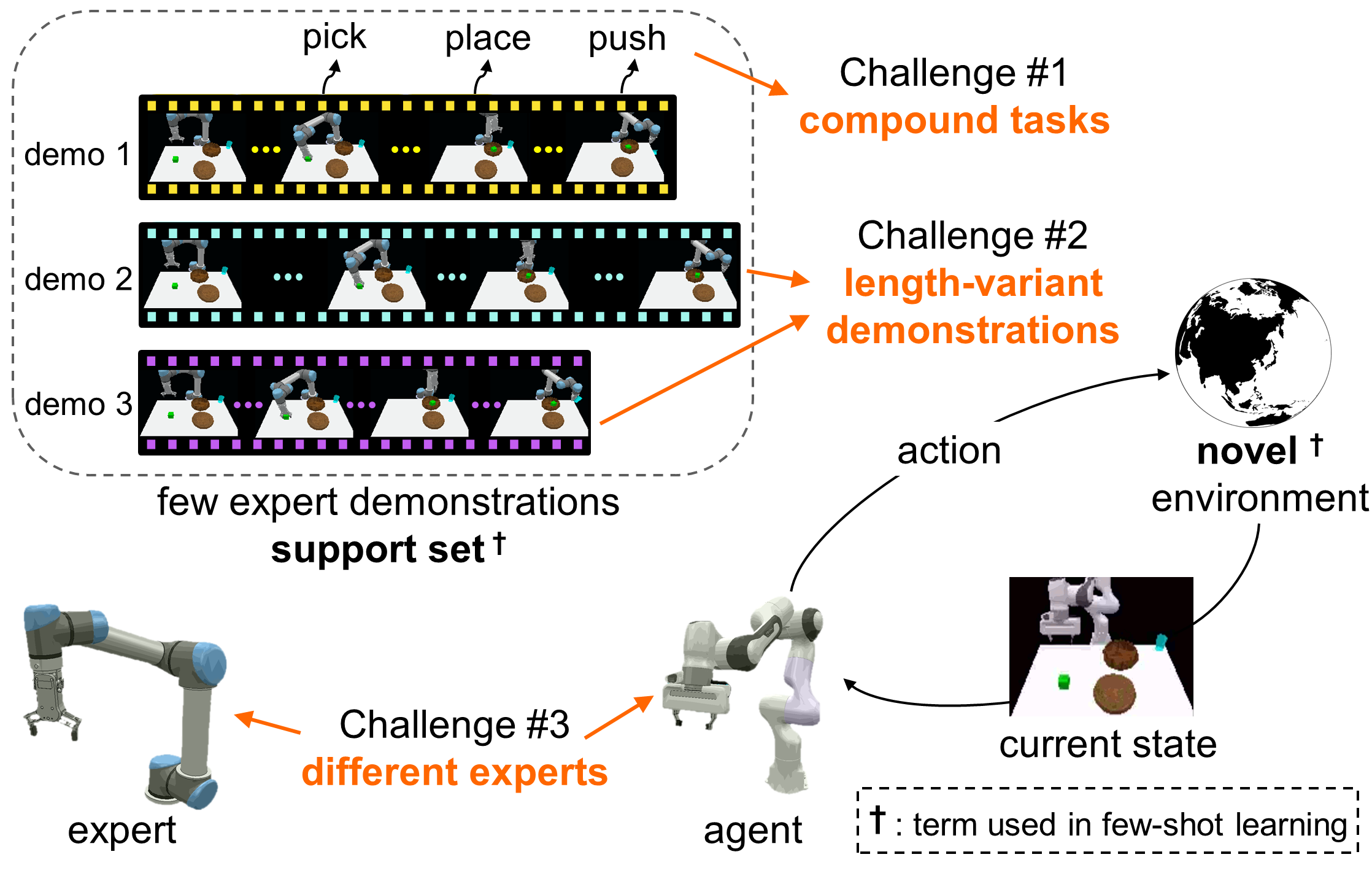
Figure 1: Schema of few-shot imitation learning (FSIL). In our FSIL problem, models need to solve the task in novel environment that is unseen during training. Few demonstrations are given to let models imitate. There are three challenges in our FSIL setting, (1) We conduct FSIL on compound tasks which contain multiple stages. (2) Demonstrations are length-variant. Each stage may locate at different timestamps. (3) Models need to learn the behavior from a different type of expert. None of previous works can solve these challenges concurrently. Moreover, learning from length-variant sequences is non-trivial, making our FSIL a challenging yet practical problem.

Meta-learning based methods (Finn et al. 2017; Yu et al. 2018, 2019) learn a meta-policy $\pi(a\mid s)$ that takes state $s$ from current playout $p$ and outputs an action $a$ via BC. Before testing, the meta-trained policy uses expert demonstrations to adapt meta-parameters. Then, they update the policy several times based on the number of demonstrations. The main drawbacks of these methods are twofold: (1) fine-tuning is required, and (2) they need a learnable loss (Yu et al. 2019) to map expert to agent explicitly.

To tackle these drawbacks, demonstration-conditioned (DC) based methods (Duan et al. 2017; James, Bloesch, and Davison 2018; Bonardi, James, and Davison 2020; Shao et al. 2020; Dasari and Gupta 2020; Dance, Perez, and Cachet 2021) apply a policy $\pi(a\mid s,\mathcal{D})$ which predict actions conditioned on both states and demonstrations $\mathcal{D}$. Fine-tuning is optional for DC methods, because they are expected to behave by observing demonstrations. They implicitly learn the mapping since they have the information in $\mathcal{D}$ concurrently when generating $a$, even if experts are different from the agent. The primary objective of DC policies is to encode few demonstrations into a representative embedding. However, it is difficult to encode length-variant demonstrations. Hence, most DC works (Duan et al. 2017; Shao et al. 2020; Dasari and Gupta 2020) only contains one demonstration in $\mathcal{D}$ and claim themselves one-shot imitation methods.

To handle demonstrations with variant lengths, some DC works apply task-embed techniques. The authors (James, Bloesch, and Davison 2018; Bonardi, James, and Davison 2020) concatenate the first and last frames of each demonstration and average their features to generate task-embedding (alias sentence in their paper). Nevertheless, this method does not consider the importance of temporal transitions that are essential for policy learning and cannot provide efficient information in the case of long demonstrations given. Therefore, Dance, Perez, and Cachet (2021) introduces a transformer-based network that considers both temporal and cross-demonstration information using attention mechanisms. They generate a task embedding by averaging the attention output of few demonstrations at each timestamp. The premise of this method is that frames at the same timestamp of each demonstration have similar knowledge. However, due to different initial states, the operating time of each stage could easily vary and result in temporal misalignment. Therefore, the model might be confused by the frame mixed with two distinct stages and degrade the performance.

We aim to design an attention mechanism that can identify important frames at different timestamp. Meanwhile, the attention mechanism should detect stages in compound tasks. A compound task containing multiple stages often appears in robotics problems. When solving compound tasks in FSIL problem, the policy needs to learn both perception and path planning. This makes solving compound tasks challenging. Yu et al. (2019) leverages an additional phase predictor to split the compound tasks, and then the policy only needs to adapt to each stage. The disadvantage is that the number of stages needs to be known in advance.

In this work, we propose a novel stage conscious attention network (SCAN). SCAN takes both demonstrations and playouts as input to learn the mapping due to the characteristic of DC method. Furthermore, SCAN applies novel stage conscious attention to let each playout frame has its attention score to each frame in the demonstrations. The frame features of demonstrations are weighted by attention scores to produce the same shape contexts. We then average them to generate the informative task-embedding. With stage conscious attention, SCAN can retrieves knowledge from few demonstrations simultaneously. Experimental results show that SCAN has a significant performance improvement compared to baselines with explainable visualizations. The overall contributions are summarized as follows:

• Our work is the first DC method that solves FSIL problem under the settings of compound task, length-variant demonstrations, and learning from a different expert.

• The novel stage conscious attention detects important frames of misalignment stages and is robust to length-variant demonstrations.

• Extensive experiment results express proposed SCAN is powerful, and explainable visualization also proves the effectiveness of novel stage conscious attention.

Related Work

Few-shot Learning.

Few-shot learning (FSL) has become popular since collecting a huge amount of labeled data is difficult in most research problems. The objective of FSL is to infer the unlabeled data (query set) by leveraging few labeled data (support set). FSL is first studied on image classification. There are many influential and well-known metric-learning-based FSL methods, such as Matching network (Vinyals et al. 2016), Prototypical network (Snell, Swersky, and Zemel 2017), and Relation Network (Sung et al. 2018). They try to learn the relationship between support and query sets rather than inferring the unlabeled data directly. Moreover, optimization-based method (Finn, Abbeel, and Levine 2017) seeks a meta-parameter set that can quickly adapt to unseen tasks. Nowadays, FSL has been extended to many research fields. For instance, image segmentation (Tian et al. 2020), object detection (Karlinsky et al. 2021), and imitation learning (Silver et al. 2020). Our work aims to develop a method that can learn unseen compound tasks with few-shot length-variant demonstrations from a different expert.

Few-shot Imitation Using RL/IRL.

Reinforcement learning (RL) methods assume the reward function of environments is known. But, it is difficult to design reward functions that give precise feedback to policies in real-world problems. Therefore, inverse RL (IRL) (Ng, Harada, and Russell 1999) infers a reward function from few expert demonstrations. Then, IRL policy can be trained by interacting with the environment under the inferred reward function. In addition, modern IRL methods (Ho and Ermon 2016; Reddy, Dragan, and Levine 2020) are usually GAN-like (Goodfellow et al. 2014). They assign a high reward to the states from demonstrations but a low reward to the states from collected agent samples. Since these methods only use rewards of states to train their model, they can handle the demonstrations without actions, which differs from BC. However, both RL and IRL methods need to interact with the target environment to train the policy. In other words, the learned reward function (IRL) or the well-trained policy (RL) do not be applicable to novel environments. In our FSIL problem, policies can only use demonstrations to fine-tune but cannot interact with the novel environment before performance evaluation. Thus, most RL and IRL methods are not available in our work.

A recent work (Dance, Perez, and Cachet 2021), named demonstration-conditioned RL (DCRL), overcomes the limitation. DCRL requires interactions with environments in training. But, it solves FSIL tasks without fine-tuning in testing. Because DCRL is a DC policy method, it needs expert demonstrations from training environments to achieve fine-tuning-free. They store the tuples of (playout history, rewards, demonstrations) into the replay buffer to train the policy. The policy is a transformer-based architecture that its encoder generates task embeddings using cross-demonstration attention and the decoder predicts the actions. Moreover, the concept of ”demonstration conditioned” echoes our motivations. But, designing all reward functions in training environments is quite time-consuming. Thus, we only compare SCAN with BC-based methods.

Compound Task.

A compound task consists of multi-stage subtasks. The main challenge of compound tasks is that there is no signal (label) in demonstrations to identify each subtask when testing. Nevertheless, the policies for distinct subtasks are pretty different. Hence, it becomes impractical to use a single policy to solve compound tasks.

An intuitive solution is to link the relationship between subtask and primitive. The term primitive, which comes from the robotics field (Flash and Hochner 2005; Manschitz et al. 2015), represents single elementary movements and is widely used in compound task problems. To be specific, each subtask may corresponds to a single robot motion (primitive), such as pushing and grasping. Therefore, previous RL (Zeng et al. 2018; Marzari et al. 2021) and IL works (Yu et al. 2019; Lee et al. 2019; Lee and Seo 2020) assume these primitives are known before testing since the end effector (gripper) are only capable for these primitives. Then, they develop a hierarchical structure that trains policies for each primitive separately and use a high-level control network to decide which policy should be executed with the current observation. Phase predictors (Yu et al. 2019) or task transition models (Lee et al. 2019; Lee and Seo 2020) are proposed to identify whether a primitive is done. Unfortunately, most of these components cannot be trained from scratch with actor networks due to the hierarchical architecture. Instead of recognizing primitives with an additional model, SCAN detects which primitive the current observation locates by an attention module. Unlike above methods, SCAN does not need to know the primitives beforehand, and all its components can be trained end-to-end.

Few-Shot Imitation Learning (FSIL)

To emphasize, we treat FSIL problem as imitation learning under FSL setting. In previous works, a policy is (trained or) tested over several tasks that are essentially the same but with different objects in the environments. Thus, we use the base environments $E^{b}$ and novel environments $E^{n}$ in problem statement. Notations are listed in Table 1.

Problem Statement

A few-shot imitation learning (FSIL) problem is given by a base environment set $E^{b}$ and a novel environment set $E^{n}$, where $E^{b}\cap E^{n}=\emptyset$. Each environment $e^{*}$ in $E^{b}$ or $E^{n}$ contains a set of expert demonstrations (support set) $\mathcal{D}^{*}$ and a set of agent playouts (query set) $\mathcal{P}^{*}$. In addition, samples in $\mathcal{D}^{*}$ or $\mathcal{P}^{*}$ are in the same environment $e^{*}$ with distinct initial/end states. Moreover, the expert could be humans or other robot arms compared to the agent in playouts.

A policy $\pi_{\theta}$ with parameter $\theta$ is meta-trained in $e^{b}$ from base environments $E^{b}$ and meta-tested in $e^{n}$ from novel environments $E^{n}$. The policy $\pi_{\theta}$ needs to generate an action $a$ when receiving a current state $s$ from the playout $p^{n}\in\mathcal{P}^{n}$. Then, the success rates of playout executions in all $e^{n}$ are used as performance evaluation. Thus, the playout samples in $e^{n}$ only contain the initial state $s_{0}$, and the following states are provided according to the action taken by the policy. At last, the objective of FSIL problem is to maximize the performance expectation of the policy where the expectation is taken over $e^{n}\in E^{n}$. Furthermore, the policy can only fine-tune its parameters using the demonstrations $\mathcal{D}^{n}$ in $e^{n}$(if needed), which means no interaction with novel environments are allowed before performance evaluation.

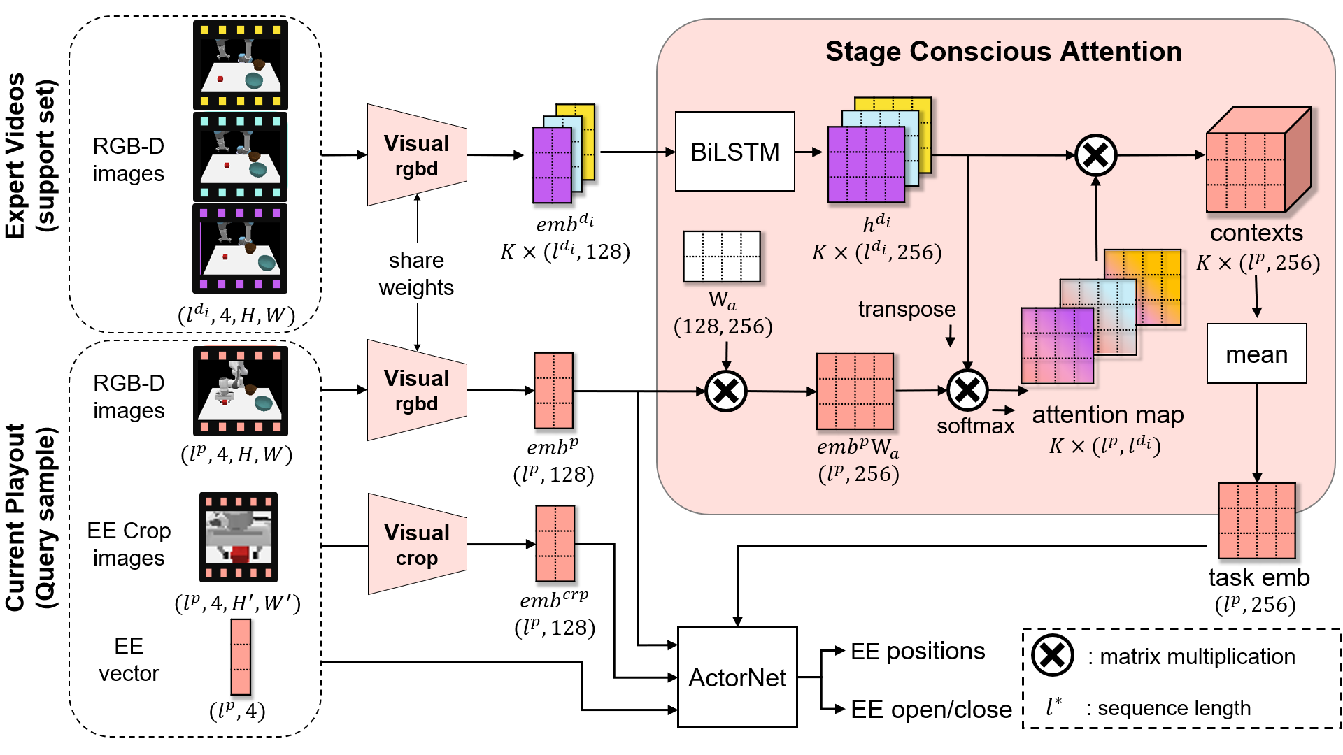
Figure 2: Architecture of stage conscious attention network (SCAN). Given a set of length-variant demonstrations (images only) and current playout data (images, end-effector (EE) cropped images, EE vector), SCAN uses a shared-weight $Visual_{rgbd}$ to extract feature embeddings (FEs) $emb^{d_{i}}$ from demonstrations and $emb^{p}$ from current playout. Meanwhile, another $Visual_{crop}$ generates FEs of EE cropped images $emb^{crp}$. Then, $emb^{d_{i}}$ are passed into a bidirectional LSTM (BiLSTM, encoder) to generate $h^{d_{i}}$ that contains time information. In addition, the attention maps are the results of matrix multiplications of $emb^{p}$ and a learnable matrix $W_{a}$ and each $h^{d_{i}}$. Afterwards, attention maps matrix multiplies by each $h^{d_{i}}$ to get contexts. Until now, length-various demonstrations are projected to same shape contexts. The task embedding (mean of contexts) contains the knowledge that each playout state focuses on. We named this process as stage conscious attention (SCA). At last, $emb^{p}$, $emb^{crp}$, ee vector and task-embeddings are fed into ActorNet (decoder) for predicting actions.

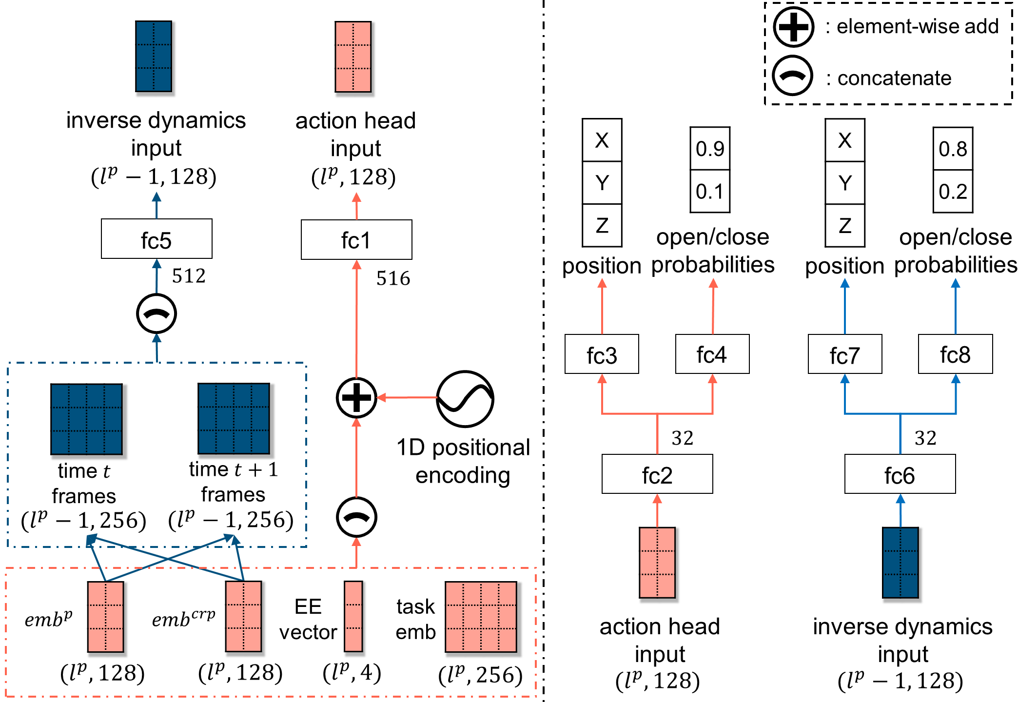
Figure 3: Architecture of ActorNet. In ActorNet, an action head concatenates four input embeddings and adds a 1D positional encoding. Following by the several dense layers,the action head computes positions and probabilities of open/close control. In the meantime, an inverse dynamics model concatenates time $t$ and $t+1$ $emb^{p}$ and $emb^{crp}$ as inputs and predict the actions using a similar architecture of action head. The inverse dynamics model helps the action head know the precise actions that cause changes between frames.

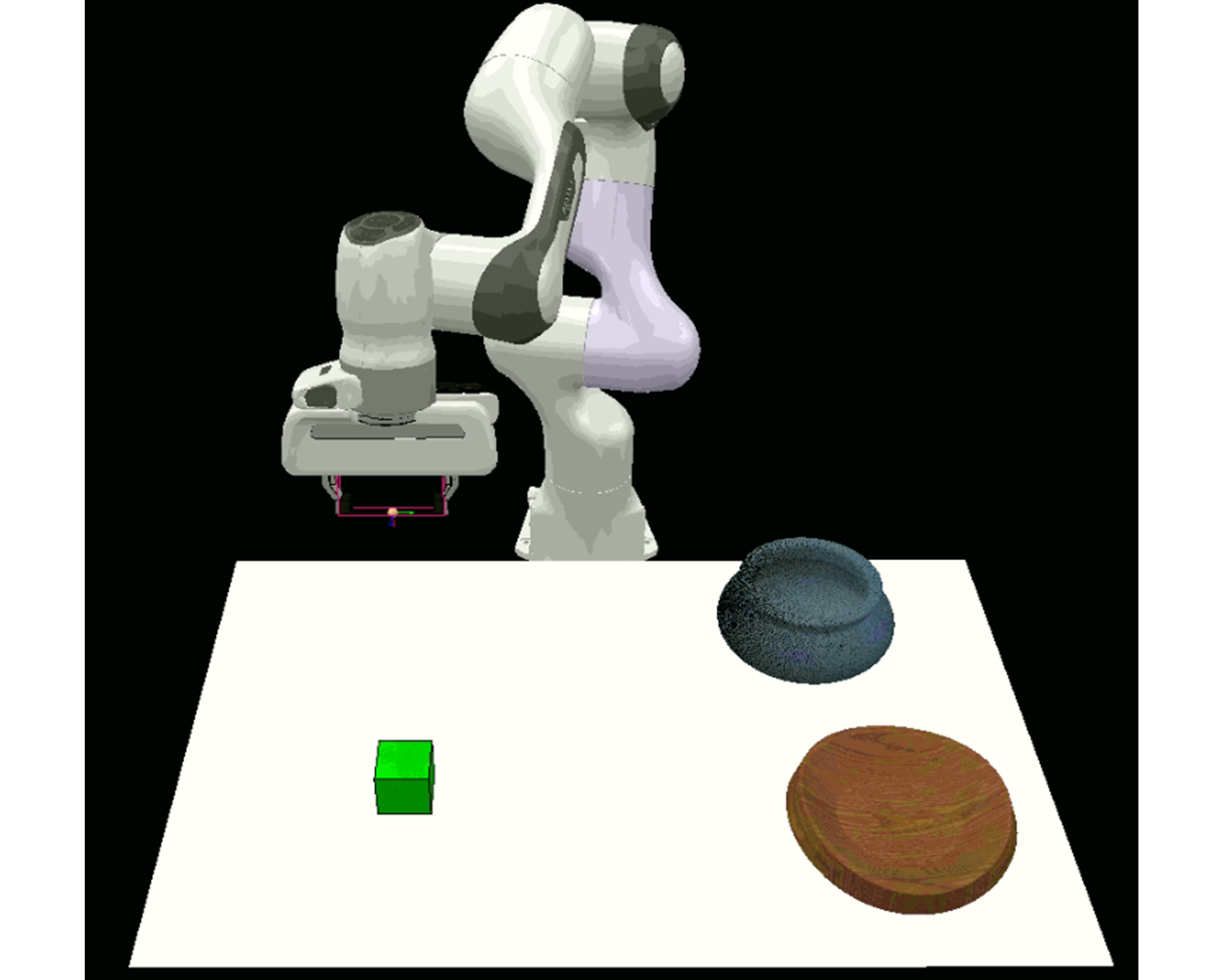
(a) pick & place (PP)

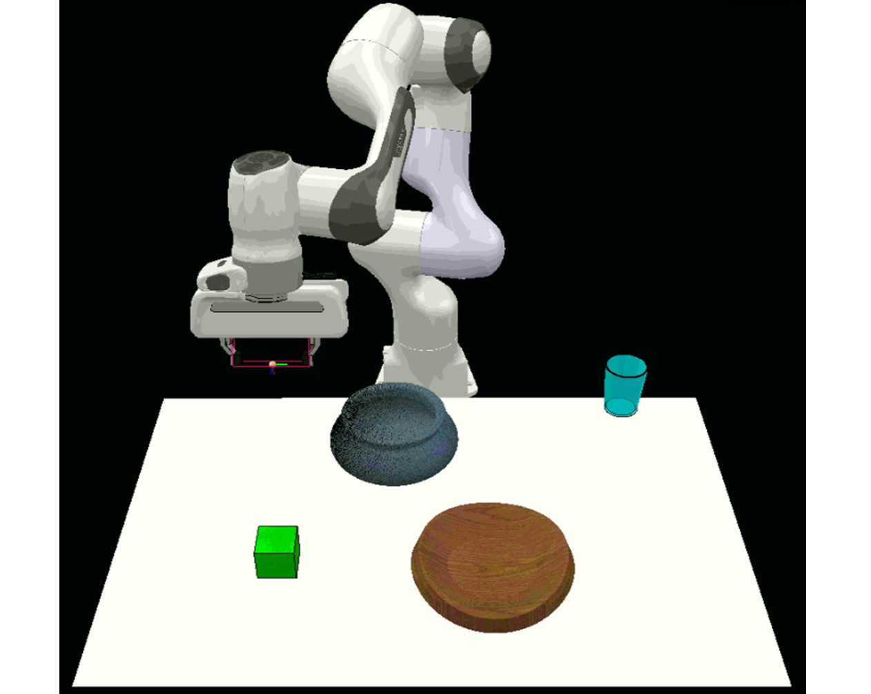
(b) pick & place & push (PPP)

Figure 4: Environments of PP and PPP task . PP and PPP task are compound tasks that contains two and three stages, respectively. Objects are unseen during training.

notation	meaning
$f,f^{crp}$	frame, crop frame
$\vec{v}$	vector
$s:=(f,f^{crp},\vec{v})$	state
$a$	action
$\mathbb{F}:=[f_{0},f_{1},...,f_{t}]$	sequence of frames
$\mathbb{F}^{crp}:=[f_{0}^{crp},f_{1}^{crp},...,f_{t}^{crp}]$	sequence of crop frames
$\vec{\mathbb{V}}:=[{\vec{v}}_{0},{\vec{v}}_{1},...,{\vec{v}}_{t}]$	sequence of vector
$\mathbb{S}:=[s_{0},s_{1},...,s_{t}]$	sequence of state
$\mathbb{A}:=[a_{0},a_{1},...,a_{t}]$	sequence of action
$p^{*}:=(\mathbb{S},\mathbb{A})^{*}$	playout
$d^{*}:=(\mathbb{F},\mathbb{A})^{*}$	demonstration
$\mathcal{P}^{*},\mathcal{D}^{*}$	set of $p^{*},d^{*}$
$e^{*}$	environment
$E^{*}$	set of $e^{*}$
${}^{*}\in\{b,n\}$	$b$: base, $n$: novel

Table 1: Defined notations

Methodology

We introduce the stage conscious attention networks (SCAN) in details. SCAN needs following inputs: $K$ expert demonstrations (without actions) $\mathcal{F}^{D}=\{\mathbb{F}^{d_{i}}\mid i\in[0,K]\}$ and playout states that contains frames $\mathbb{F}^{p}$, end-effector (EE) cropped frames $\mathbb{F}^{crp}$, and EE vector $\vec{\mathbb{V}}^{p}$ (position and open amount). These inputs are widely used in FSIL works. Moreover, we apply inverse kinematics to compute joint parameters of the agent. Therefore, SCAN only needs to compute two outputs for each playout state: target positions (x, y, z in continuous space) and the probabilities for EE open/closing. SCAN is composed of three main components, including visual heads, stage conscious attention, and an ActorNet. We describe these components in following paragraphs, and the overall architecture of SCAN is shown in Figure 2.

Visual Head.

The objective of visual head is to retrieve meaningful embeddings of RGB-D frames either from $\mathcal{F}^{D}$ or $\mathbb{F}^{p}$. We leverage two resnet18 to extract RGB images and depth images separately, inspired by (Shao et al. 2020). Moreover, since SCAN does not have object detection components, we insert a modified self-attention module at the head and tail of resnet18. The self-attention module is originally proposed in (Zhang et al. 2019), we make the output dimension of the query-layer and key-layer the same as input dimensions and add the channel-wise softmax layer behind them. Detailed architecture is shown in supplementary.

Then, given a 4D frame inputs (sequence length $l^{p}$ for $\mathbb{F}^{p}$ or $l^{d_{i}}$ for $\mathbb{F}^{d_{i}}$, channel $C$, height $H$, width $W$), the visual head splits it into RGB and depth images and use the corresponding resnet18 to generate feature embeddings (FEs). These two FEs are concatenated and passed over a dense layer to obtain the output with shape ($l^{p}$ or $l^{d_{i}}$, 128). As shown in Figure 2, a shared-weights $Visual_{rgbd}$ extracts $emb^{p}$ from $\mathbb{F}^{p}$ and each $emb^{d_{i}}$ from $\mathbb{F}^{d_{i}}$. Another $Visual_{crop}$ extracts $emb^{crp}$ from $\mathbb{F}^{crp}$.

Stage Conscious Attention (SCA).

We assume that each frames in each demonstration $\mathbb{F}^{d_{i}}$ (support sample) has a different importance to each frame in playout $\mathbb{F}^{p}$ (query sample). Unlike the cross-demonstration attention (temporal-awareness attention) in (Dance, Perez, and Cachet 2021), SCAN leverages a stage conscious attention that lets each frame of current playout has its own interpretation of each demonstration. The overall structure is shown in Fig. 2.

We feed each $emb^{d_{i}}$ into a bidirectional LSTM (BiLSTM) to obtain $h^{d_{i}}$ that contains temporal information. Then, the general form of global attention motivated by (Luong, Pham, and Manning 2015) is applied to generate an attention map $attn^{p}_{d_{i}}$ between $h^{d_{i}}$ and FEs of playout $emb^{p}$. To be specific, $attn^{p}_{d_{i}}$ is the result of matrix multiplied of $emb^{p}$ and a learnable matrix $W_{a}$ and $h^{d_{i}}$. The $W_{a}$ makes sure the $emb^{p}$ has a same latent size of $h^{d_{i}}$, which is useful when dealing with two different shape matrix. Then, a $softmax$ layer makes each row (attention scores at each frame in the demonstration $d_{i}$ given by each frame in current playout) of attention map are summed to 1. Next, the context $c^{d_{i}}$ is the result of matrix multiplication of $attn^{p}_{d_{i}}$ and each $h^{d_{i}}$. At last, the task-embedding $emb^{task}$ is the mean of $K$ contexts $c^{d_{i}}$.

$$attn_{d_{i}}^{p}=softmax(emb^{p}W_{a}(h^{d_{i}})^{T})$$

$$c^{d_{i}}=attn_{d_{i}}^{p}\cdot h^{d_{i}}$$

ActorNet.

ActorNet predicts actions in continuous space rather than discrete spaces. It allows the agent to perform more precise actions. The overall picture of ActorNet is shown in Figure 3. In ActorNet, there are two components, action head and inverse dynamics model. The action head concatenates four inputs ($emb^{p}$, $emb^{crp}$, EE vector $\vec{\mathbb{V}}^{p}$, $emb^{task}$) and add 1D positional encoding $PE_{1D}$ to provide auxiliary time information. Then the action head predicts target positions and probability of open/close for each state in current playout (history), we denote the output as $out_{act}$.

$$in_{act}=PE_{1D}([emb^{p};emb^{crp};\vec{\mathbb{V}}^{p};emb^{task}])$$

The $out_{act}$ is a vector of pairs $[\vec{\mu}_{t},g_{t}]$ for the time $t$ state in the playout history. The $\vec{\mu}_{t}=[\mu_{x},\mu_{y},\mu_{z}]$ is a vector which contains means of three uni-variate Gaussian distributions that generate positions at time $t$. We use an additional learnable vector $\vec{\sigma}$ for the standard deviation of the distributions. Besides, the $g_{t}$ is the probability of open/close control.

Afterwards, the inverse dynamic model concatenates time $t$ $emb^{p}$, $emb^{crp}$ and time $t+1$ $emb^{p}$, $emb^{crp}$ as input $in_{inv}$, and use the similar architecture of action head to predict actions $out_{inv}$ for each state in playout history (except for the latest frame). The inverse dynamic model aims to help the action head know how actions cause frame changes.

$$in_{inv}=[[emb^{p}_{t},emb^{crp}_{t}],[emb^{p}_{t+1},emb^{crp}_{t+1}]]$$

To train SCAN, we use negative-log-likelihood (NLL) as loss functions. $L_{*}^{pos}$ calculates the NLL loss for the output $out_{*}$ of the predicted positions. Besides, $*$ could be $act$ or $inv$. And the $\vec{a}=[a_{x},a_{y},a_{z}]$ is the vector of labeled actions.

$$L_{*}^{pos}=-\frac{1}{K}\sum_{i=1}^{K}\sum_{j\in[x,y,z]}\frac{1}{2}\ln(2\pi)+\ln(\vec{\sigma}_{j})+\frac{(a_{j}-\mu_{j})^{2}}{2\sigma_{j}^{2}}$$

We use the following loss for open/close control. The $g^{label}\in\{0,1\}$ is true probability of open the gripper. And, $*$ indicates action head $act$ or inverse dynamics model $inv$.

$$L_{*}^{g}=-\frac{1}{K}\sum_{i=1}^{K}g^{label}\ln{g}+(1-g^{label})\ln(1-g)$$

The total loss is the weighted sum of all losses, and $\lambda^{pos}$, $\lambda^{g}$ are the hyper-parameters.

$$L_{total}=\lambda^{pos}(L_{act}^{pos}+L_{inv}^{pos})+\lambda^{g}(L_{act}^{g}+L_{inv}^{g})$$

Experiments

The goal of our experiments is to verify following assumptions: (1) the novel stage conscious attention has the ability to locate each primitive (stage) in length-variant demonstrations and highlight important frames for each playout frame. (2) SCAN can learn a relationship mapping between different types of experts and agent. (3) Based on above assumptions, SCAN can retrieve knowledge from few demonstrations simultaneously and get a boosted performance rather than separately handling each demonstration.

Experiment Settings.

We have two main experiments. (1) we evaluate all methods on two compound tasks, pick & place (PP) and pick & place & push (PPP), as shown in Figure 4. In PP task (2 stages), the agent needs to pick the cube and place it in the target bowl. Another bowl serves as the disruptor. Next, in PPP task (3 stages), the agent needs to push the sky-blue cup off the table after placing the cube. Note that the target bowl might be the front one or rear one. This means the directions of the trajectory are quite different, which makes our experiment challenging. Moreover, we follow the evaluation protocol in FSL problem. There are 56 novel environments composed of unseen objects. For each environment, we let methods play 20 times with different initial scenes and calculate the success rate. The average of successful rate and standard deviation in all novel environments are provided in Table 2. This experiment aims to evaluate whether SCAN can locate important frames and achieve dominating performance. (2) We design a extremely length-biased case to observe the robustness of methods when encountering sub-optimal demonstrations (still complete the task but with trivial moves) that have not been processed. To be clear, all methods are trained with optimal demonstrations. Then, we give few sub-optimal demonstrations in testing to analyze the relation between attention mechanism and performance changes, as shown in Figure 7 and 8. For all experiments, we build environments in CoppeliaSim and use the pyrep (James, Freese, and Davison 2019) toolkit to communicate with environments. We use Panda arm as the agent, and experts may be Panda arm or UR5.

Type	Models	Fine-tune	PP task		PPP task
			1-shot	5-shot	1-shot	5-shot
same	BC		01.70% $\pm$ 03.31%		03.30% $\pm$ 4.04%
	meta-BC	✓	12.86% $\pm$ 12.74%	28.84% $\pm$ 09.82%	05.54% $\pm$ 09.76%	28.57% $\pm$ 12.67%
	TaskEmb (2018)		35.09% $\pm$ 34.99%	34.11% $\pm$ 34.50%	17.77% $\pm$ 18.47%	18.39% $\pm$ 19.66%
		✓	54.20% $\pm$ 25.74%	83.39% $\pm$ 13.47%	47.23% $\pm$ 18.85%	58.39% $\pm$ 18.49%
	TANet (ours)		28.75% $\pm$ 14.24%	40.75% $\pm$ 12.37%	46.43% $\pm$ 21.69%	48.13% $\pm$ 18.79%
		✓	53.93% $\pm$ 20.54%	64.82% $\pm$ 15.84%	52.05% $\pm$ 21.04%	68.57% $\pm$ 14.16%
	SCAN (ours)		67.05% $\pm$ 21.31%	75.45% $\pm$ 17.66%	46.34% $\pm$ 13.18%	47.86% $\pm$ 13.69%
		✓	64.64% $\pm$ 21.50%	85.00% $\pm$ 10.69%	55.80% $\pm$ 20.24%	58.48% $\pm$ 22.56%
differ	meta-BC	✓	06.52% $\pm$ 09.95%	05.80% $\pm$ 08.17%	00.00% $\pm$ 00.00%	00.00% $\pm$ 00.00%
	TaskEmb (2018)		18.04% $\pm$ 09.81%	18.66% $\pm$ 09.61%	12.32% $\pm$ 14.70%	12.23% $\pm$ 15.12%
	TANet (ours)		42.50% $\pm$ 14.82%	47.95% $\pm$ 14.63%	24.02% $\pm$ 26.30%	25.54% $\pm$ 27.20%
	SCAN (ours)		60.89% $\pm$ 14.70%	65.27% $\pm$ 13.74%	31.52% $\pm$ 10.60%	32.41% $\pm$ 11.38%

Table 2: Success rate on compound tasks. The average of success rate and standard deviation in all novel environments are provided. The type column represents whether the expert and the agent are the same or not. In the same expert setting, model can fine-tune when expert actions are provided. From the table, we have three main findings. (1) the 5-shot performance usually outperforms the 1-shot performance. (2) fine-tuning is helpful in most cases, but it might let model overfit on the demonstration in one-shot setting. (3) SCAN has the best adaptation ability and performance except for the case of same expert in PPP task.

Compared Baselines.

Baselines are introduced below. All methods use our visual head and ActorNet for fair comparisons. Only the parts that handle few demonstrations are implemented. (1) BC: a conventional BC model takes states as input, no task-embedding generated. (2) meta-BC: a conventional BC is trained via MAML (Finn, Abbeel, and Levine 2017) in same expert setting and trained via DAML (Yu et al. 2018) in different expert setting. (3) TaskEmb: a DC method (James, Bloesch, and Davison 2018) averages concatenated embeddings of first and last frames as task-embeddings.(4) TANet: our implemented DC method that averages the output of cross-demonstration attention (at each timestamp) and apply the global attention to get the task-embeddings. The key idea of TANet is similar to the method in (Dance, Perez, and Cachet 2021), however, it is hard to build a transformer-based model with our visual head and ActorNet. Therefore, we design the TANet to evaluate the effectiveness of cross-demonstration attention.

Performance Comparison

We analyze the performance results of experiment 1 in Table 2. The success rate and standard deviation is the average of 56 novel environments. We have several observations from the results. (1) Except for TaskEmb, methods achieve better performance in 5-shot setting rather than 1-shot setting. TaskEmb only uses frame features when generating task-embedding, and there is no other conversion process. Therefore, it is susceptible to frame features from novel environments. Without fine-tuning, TaskEmb performance of 1-shot and 5-shot is not much different. (2) The performance of DC methods has been dramatically improved after fine-tuning. But SCAN has slightly worse performance in PP task under the 1-shot setting. We infer that using only one demonstration to fine-tune may let models overfit. Therefore, the generalization of models is reduced. (3) SCAN has the best adaptability in most cases, regardless of whether the expert is the same as the agent. We claim that the proposed SCA learns the mapping from demonstration to playout. And, the learned mapping can provide enough information for SCAN to behave in a novel environment even without fine-tuning.

Furthermore, we also observe an interesting phenomenon. TANet has trouble in PP task, even with fine-tuning. Because the time misalignment between demonstrations in PP tasks is serious, averaging information at each timestamp like TANet causes the task to be incomprehensible. Our SCAN identifies the location of critical frames in demonstrations. Therefore, SCAN can learn and behave smoothly in PP task. However, TANet outperforms SCAN in the PPP task under the same expert setting. We infer two possible reasons regarding this phenomenon: (1) Although demonstrations of PPP task have longer lengths and more steps, their time misalignment are not severe. (2) Bowls are at the front of the agent, and many bowls have similar colors to the agent in novel environments, which interferes with SCAN that needs to pay attention to each frame.

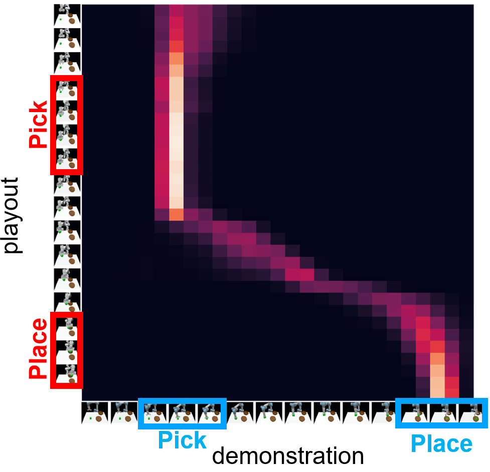
(a) PP task (2 primitives)

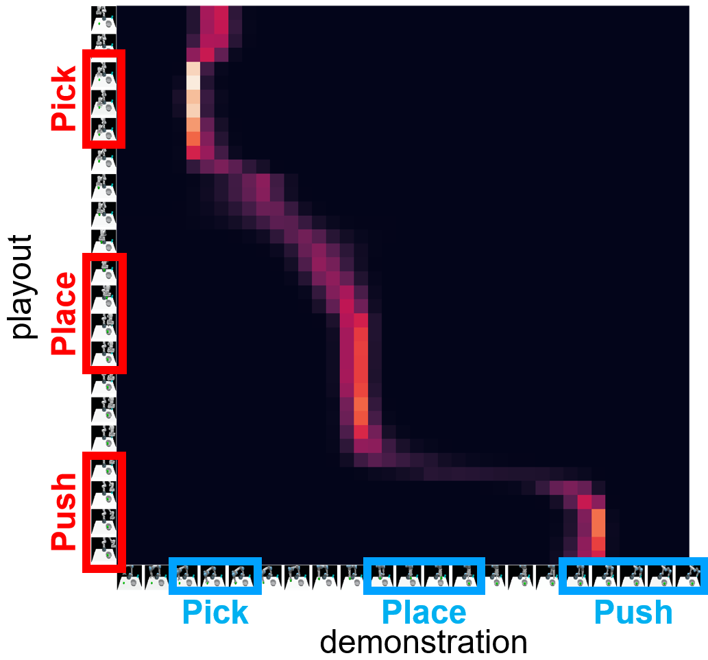
(b) PPP task (3 primitives)

Figure 5: Attention maps of SCAN on compound tasks. Each row and column represent the frame from the playout and the demonstration. Besides, a lighter cell has a higher score, and we mark each primitive with the same color. The attention results show that SCAN can focus on corresponding frames (beginning of same stage) in the demonstration when executing each stage (in both tasks).

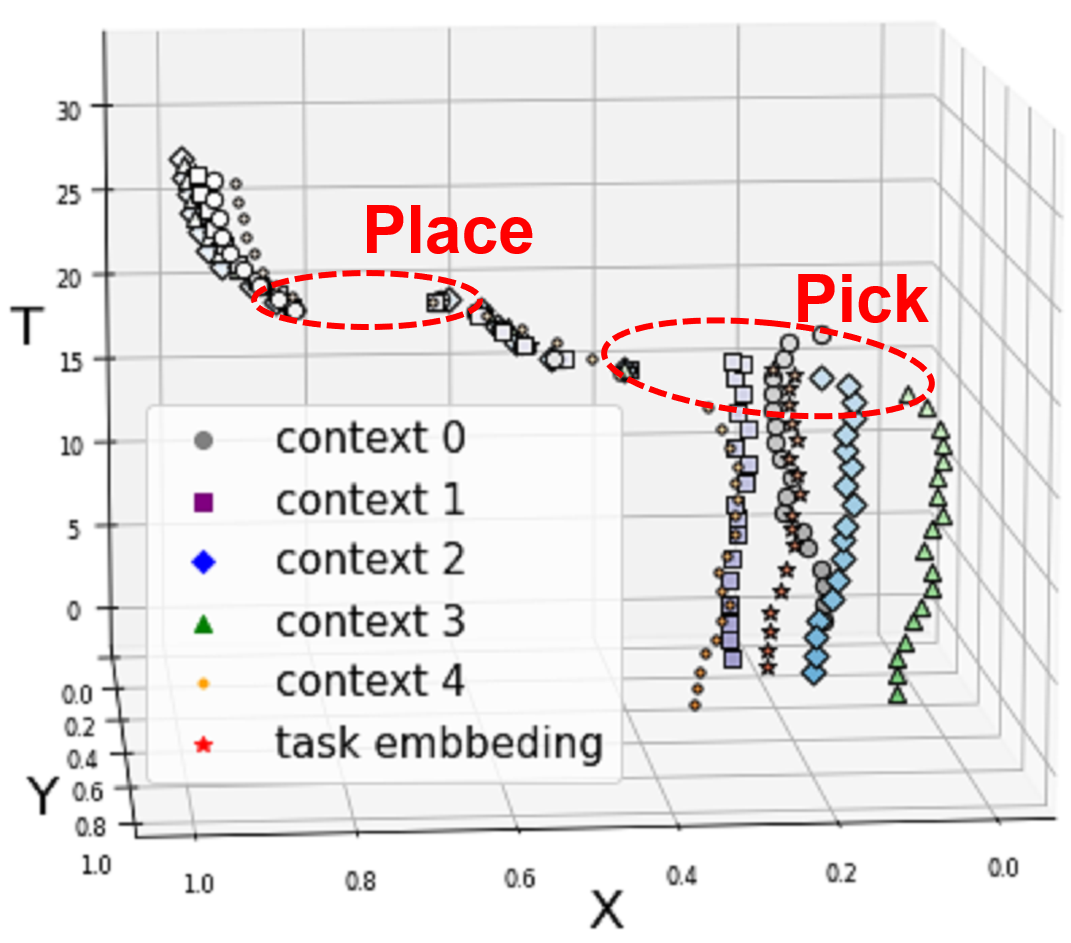
(a) PP task (2 primitives)

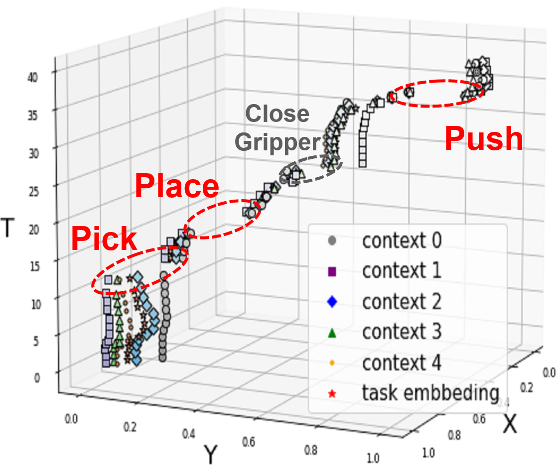
(b) PPP task (3 primitives)

Figure 6: t-SNE of SCAN contexts. The X, Y axes are the projection of t-SNE, and the T-axis represents the timestamp. A context at time $t$ (datapoint at $(x,y,t)$) is generated by time $t$ playout frame and a demonstration. Besides, contexts from different demonstrations are tagged with distinct marker. We illustrate how the relationship between contexts changes over time. Since initial states of demonstrations are various, the contexts are diverse. Surprisingly, contexts aggregate after primitives are executed, which implies that the contexts indeed contain the task-related knowledge.

Effectiveness of Stage Conscious Attention (SCA)

Attention Result in Compound Tasks.

To verify whether SCA can detect crucial frames and generate informative task-embedding, Figure 5 and Figure 6 visualize attention maps and contexts generated by SCA in the compound tasks of experiment 1. To emphasize, all visualizations are under the setting of 5-shot and different experts. In Figure 5, attention scores of the stage where the agent is in progress focus on the same stage in demonstrations, whether the compound task has 2 or 3 stages. Notably, SCA locate critical frames in novel environments without fine-tuning. Furthermore, we do not use any hard restriction or loss function to guide SCA. It learns the ability proactively. On the other hand, Figure 6 illustrates t-SNE (van der Maaten and Hinton 2008) results of contexts and task-embeddings in the playout of Figure 5. The contexts come from different demonstration are tagged with distinct marker. In addition, we highlight stage locations in t-SNE results. At the beginning, generated contexts and task-embeddings are diverse since the initial states of demonstrations are various. Specially, contexts aggregate when each stage is over. The rest of contexts are generated during moving, such as moving to target cubes or bowls. It is impressive that contexts have these cluster attributes.

Robustness to Sub-optimal Demonstrations.

Figure 7 and Figure 8 demonstrate the result of experiment 2. We choose one from 56 novel environments as the target environment and generate the sub-optimal demonstrations. Experts still completed the task in sub-optimal demonstrations but with trivial movements. In other words, the demonstration set is extremely length-biased, which all methods have never encountered during training. Then, we run all methods 20 times for the performance evaluation. Attention maps of SCAN and TANet baseline in this experiment are shown in Figure 7. It is the comparison with zero or three sub-optimal demonstrations in the demonstration set. Both methods work well when there are no sub-optimal demonstrations (bottom). However, TANet cannot handle the case that there are three sub-optimal demonstrations (top). Because the time misalignment is severe in the case, TANet is hard to retrieve knowledge by averaging at each timestamp of demonstrations, which can be reflected in success rates of Figure 8.

In Figure 8, TANet performs poorly when the number of sub-optimal demonstrations increases. Our SCAN is also affected by sub-optimal demonstrations, but it did not cause such a big reduction in performance. Moreover, TaskEmb only focuses on first and last frames of demonstrations, and thus, sub-optimal demonstrations would not affect its performance. However, first and last frames cannot provide efficient information when solving compound tasks, TaskEmb has a lower performance compared to other methods.

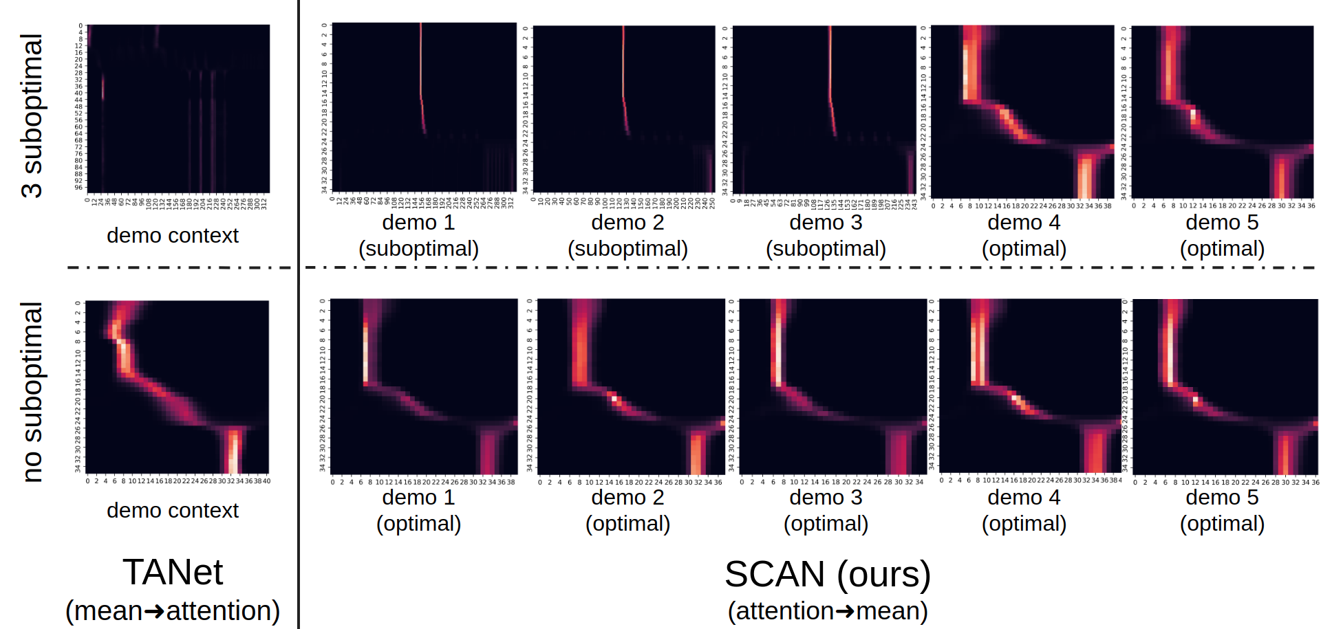
Figure 7: Attention in extremely length-biased case. Methods are trained with optimal demonstrations, but the demonstration set contains sub-optimal demonstrations (with trivial moves) in testing. When there are all optimal demonstrations, both TANet and SCAN can find important frames. However, the attention result of TANet becomes a mess when there are 3 sub-optimal demonstrations. Because TANet averages attention by each timestamp, the information are mixed and hard to retrieve. By contrast, SCAN generates attention to each demonstration individually and then averages the results. Since unimportant frames has been filtered out, SCAN can still extract important information.

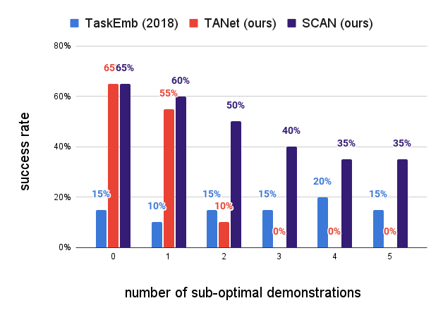
Figure 8: Model robustness in extremely length-biased case. We analyze the relation between success rate and the number of sub-optimal demonstrations. TANet cannot handle sub-optimal demonstrations since they average attention by timestamp. Its performance dramatically decreases while the number of sub-optimal demonstrations increases. In the contrary, our SCAN is more robust to the demonstrations with extremely different length. TaskEmb only considers the first and last frame, therefore, it does not matter in this case.

Conclusion

In this work, we conduct the FSIL problem under three challenging settings, including compound tasks, few length-variant demonstrations and learning from a different expert. Meanwhile, we found that most of works can only handle one demonstration at once or need external loss to learn from different experts. Hence, we propose a novel SCAN method that can retrieve knowledge from few demonstrations simultaneously and behave in novel environments without fine-tuning. Our stage conscious attention locates critical frames for each playout frame to alleviate the demonstration misalignment problem. Explainable visualization and outstanding performance illustrates the effectiveness of SCAN.

See pages - of supp.pdf

References

- Bonardi, James, and Davison (2020) Bonardi, A.; James, S.; and Davison, A. J. 2020. Learning One-Shot Imitation From Humans Without Humans. IEEE Robotics and Automation Letters, 5(2): 3533–3539.
- Dance, Perez, and Cachet (2021) Dance, C. R.; Perez, J.; and Cachet, T. 2021. Demonstration-Conditioned Reinforcement Learning for Few-Shot Imitation. In Proceedings of the 38th International Conference on Machine Learning, volume 139, 2376–2387.
- Dasari and Gupta (2020) Dasari, S.; and Gupta, A. 2020. Transformers for One-Shot Imitation Learning. In CoRL 2020.
- Duan et al. (2017) Duan, Y.; Andrychowicz, M.; Stadie, B.; Jonathan Ho, O.; Schneider, J.; Sutskever, I.; Abbeel, P.; and Zaremba, W. 2017. One-Shot Imitation Learning. In Advances in Neural Information Processing Systems, volume 30.
- Finn, Abbeel, and Levine (2017) Finn, C.; Abbeel, P.; and Levine, S. 2017. Model-Agnostic Meta-Learning for Fast Adaptation of Deep Networks. In Proceedings of the 34th International Conference on Machine Learning, volume 70, 1126–1135.
- Finn et al. (2017) Finn, C.; Yu, T.; Zhang, T.; Abbeel, P.; and Levine, S. 2017. One-Shot Visual Imitation Learning via Meta-Learning. In CoRL 2017, 357–368.
- Flash and Hochner (2005) Flash, T.; and Hochner, B. 2005. Motor Primitives in Vertebrates and Invertebrates. Current Opinion in Neurobiology, 15(6): 660–666. Motor sytems / Neurobiology of behaviour.
- Goodfellow et al. (2014) Goodfellow, I.; Pouget-Abadie, J.; Mirza, M.; Xu, B.; Warde-Farley, D.; Ozair, S.; Courville, A.; and Bengio, Y. 2014. Generative Adversarial Nets. In Advances in Neural Information Processing Systems, volume 27.
- Ho and Ermon (2016) Ho, J.; and Ermon, S. 2016. Generative Adversarial Imitation Learning. In Advances in Neural Information Processing Systems, volume 29.
- James, Bloesch, and Davison (2018) James, S.; Bloesch, M.; and Davison, A. J. 2018. Task-Embedded Control Networks for Few-Shot Imitation Learning. In CoRL 2018.
- James, Freese, and Davison (2019) James, S.; Freese, M.; and Davison, A. J. 2019. PyRep: Bringing V-REP to Deep Robot Learning. arXiv preprint arXiv:1906.11176.
- Karlinsky et al. (2021) Karlinsky, L.; Shtok, J.; Alfassy, A.; Lichtenstein, M.; Harary, S.; Schwartz, E.; Doveh, S.; Sattigeri, P.; Feris, R.; Bronstein, A.; and Giryes, R. 2021. StarNet: towards Weakly Supervised Few-Shot Object Detection. In Proceedings of AAAI, volume 35, 1743–1753.
- Lee and Seo (2020) Lee, S.-H.; and Seo, S.-W. 2020. Learning Compound Tasks without Task-specific Knowledge via Imitation and Self-supervised Learning. In Proceedings of ICML, volume 119, 5747–5756.
- Lee et al. (2019) Lee, Y.; Sun, S.-H.; Somasundaram, S.; Hu, E. S.; and Lim, J. J. 2019. Composing Complex Skills by Learning Transition Policies. In Proceedings of ICLR.
- Luong, Pham, and Manning (2015) Luong, M.-T.; Pham, H.; and Manning, C. D. 2015. Effective Approaches to Attention-based Neural Machine Translation. arXiv:1508.04025.
- Manschitz et al. (2015) Manschitz, S.; Kober, J.; Gienger, M.; and Peters, J. 2015. Learning Movement Primitive Attractor Goals and Sequential Skills from Kinesthetic Demonstrations. Robotics and Autonomous Systems, 74: 97–107.
- Marzari et al. (2021) Marzari, L.; Pore, A.; Dall’Alba, D.; Aragon-Camarasa, G.; Farinelli, A.; and Fiorini, P. 2021. Towards Hierarchical Task Decomposition using Deep Reinforcement Learning for Pick and Place Subtasks. arXiv, abs/2102.04022.
- Ng, Harada, and Russell (1999) Ng, A. Y.; Harada, D.; and Russell, S. 1999. Policy invariance under reward transformations: Theory and application to reward shaping. In Proceedings of ICML, 278–287.
- Reddy, Dragan, and Levine (2020) Reddy, S.; Dragan, A. D.; and Levine, S. 2020. SQIL: Imitation Learning via Reinforcement Learning with Sparse Rewards. In ICLR.
- Shao et al. (2020) Shao, Q.; Qi, J.; Ma, J.; Fang, Y.; Weiming, W.; and Hu, J. 2020. Object Detection-Based One-Shot Imitation Learning with an RGB-D Camera. Applied Sciences, 10: 803.
- Silver et al. (2020) Silver, T.; Allen, K. R.; Lew, A. K.; Pack Kaelbling, L.; and Tenenbaum, J. 2020. Few-Shot Bayesian Imitation Learning with Logical Program Policies. Proceedings of the AAAI Conference on Artificial Intelligence, 34(06): 10251–10258.
- Snell, Swersky, and Zemel (2017) Snell, J.; Swersky, K.; and Zemel, R. 2017. Prototypical Networks for Few-shot Learning. In Advances in Neural Information Processing Systems 30, 4077–4087.
- Sung et al. (2018) Sung, F.; Yang, Y.; Zhang, L.; Tao Xiang, P. H. T.; and Hospedales, T. M. 2018. Learning to Compare: Relation Network for Few-Shot Learning. In IEEE/CVF Conference on Computer Vision and Pattern Recognition, 1199–1208.
- Tian et al. (2020) Tian, P.; Wu, Z.; Qi, L.; Wang, L.; Shi, Y.; and Gao, Y. 2020. Differentiable Meta-Learning Model for Few-Shot Semantic Segmentation. In Proceedings of AAAI, 12087–12094.
- van der Maaten and Hinton (2008) van der Maaten, L.; and Hinton, G. 2008. Visualizing Data using t-SNE. Journal of Machine Learning Research, 9(86): 2579–2605.
- Vinyals et al. (2016) Vinyals, O.; Blundell, C.; Lillicrap, T.; kavukcuoglu, k.; and Wierstra, D. 2016. Matching Networks for One Shot Learning. In Advances in Neural Information Processing Systems 29, 3630–3638.
- Yu et al. (2019) Yu, T.; Abbeel, P.; Levine, S.; and Finn, C. 2019. One-Shot Composition of Vision-Based Skills from Demonstration. In 2019 IEEE/RSJ International Conference on Intelligent Robots and Systems (IROS), 2643–2650.
- Yu et al. (2018) Yu, T.; Finn, C.; Dasari, S.; Xie, A.; Zhang, T.; Abbeel, P.; and Levine, S. 2018. One-Shot Imitation from Observing Humans via Domain-Adaptive Meta-Learning. In Robotics: Science and Systems (RSS).
- Zeng et al. (2018) Zeng, A.; Song, S.; Welker, S.; Lee, J.; Rodriguez, A.; and Funkhouser, T. 2018. Learning Synergies Between Pushing and Grasping with Self-Supervised Deep Reinforcement Learning. In 2018 IEEE/RSJ International Conference on Intelligent Robots and Systems (IROS), 4238–4245.
- Zhang et al. (2019) Zhang, H.; Goodfellow, I.; Metaxas, D.; and Odena, A. 2019. Self-Attention Generative Adversarial Networks. arXiv:1805.08318.