Achieving Carnot efficiency in a finite-power Brownian Carnot cycle with arbitrary temperature difference

Abstract

Achieving the Carnot efficiency at finite power is a challenging problem in heat engines due to the trade-off relation between efficiency and power that holds for general heat engines. It is pointed out that the Carnot efficiency at finite power may be achievable in the vanishing limit of the relaxation times of a system without breaking the trade-off relation. However, any explicit model of heat engines that realizes this scenario for arbitrary temperature difference has not been proposed. Here, we investigate an underdamped Brownian Carnot cycle where the finite-time adiabatic processes connecting the isothermal processes are tactically adopted. We show that in the vanishing limit of the relaxation times in the above cycle, the compatibility of the Carnot efficiency and finite power is achievable for arbitrary temperature difference. This is theoretically explained based on the trade-off relation derived for our cycle, which is also confirmed by numerical simulations.

I Introduction

In recent years, understanding the relation between efficiency and power in heat engines has been recognized as an important issue in nonequilibrium thermodynamics. The Carnot efficiency $\eta_{\rm C}$ gives the upper bound of the efficiency $\eta$ of any heat engine operating between hot and cold heat baths with the temperature $T_{h}$ and $T_{c}(<T_{h})$,

$$\eta\leq\eta_{\rm C}\equiv 1-\frac{T_{c}}{T_{h}},$$ (1)

where $\eta$ is defined as the ratio of the work to the heat from the hot heat bath [1, 2]. The Carnot efficiency can usually be realized in the quasistatic Carnot cycle that takes an infinitely long cycle time. However, the power $P$ defined as the output work per unit time vanishes in the quasistatic limit. Since the compatibility of the Carnot efficiency and finite power may not be forbidden by the second law of thermodynamics, many efforts have been made to achieve it [3, 4, 5, 6, 5, 7, 8, 9, 10, 11, 12, 13, 14, 15, 16, 17, 18, 19, 20]. This possibility, however, may be reconsidered in terms of the recently formulated trade-off relation between the efficiency and power in heat engines [21, 22, 23, 24, 25],

$$P\leq A\eta(\eta_{\rm C}-\eta),$$ (2)

where $A$ is a positive quantity depending on the system. Applicability of the trade-off relation ranges from macroscopic heat engines [21] to stochastic ones [22, 23, 24, 25] described by the Markovian dynamics. According to this relation, as the efficiency $\eta$ approaches $\eta_{\rm C}$, the power vanishes, which means that the compatibility of the Carnot efficiency and finite power is forbidden.

On the other hand, if the quantity $A$ in Eq. (2) diverges at the same time as $\eta$ approaches $\eta_{\rm C}$, the power may remain finite. By focusing on the dependence of $A$ on the relaxation times, Holubec and Ryabov proposed a scenario to achieve the Carnot efficiency at finite power without breaking the trade-off relation by taking the vanishing limit of the relaxation times, which can yield a diverging quantity $A$ [17]. However, complicated dependence of the quantity $A$ and the efficiency $\eta$ on the relaxation times may make the feasibility of the scenario nontrivial.

In Ref. [18], we studied the Brownian Carnot cycle to demonstrate the feasibility of the above scenario. We used an underdamped Brownian Carnot cycle, where the instantaneous change of the potential and temperature of the heat bath is used as an adiabatic process [17, 26, 27, 28]. We numerically and theoretically showed the compatibility of the Carnot efficiency and finite power in the vanishing limit of the relaxation times in the small temperature-difference regime. This result was obtained by explicitly expressing the relaxation-times dependence of $A$ and $\eta$ in Eq. (2). In the large temperature-difference regime, however, we cannot achieve the compatibility even in the vanishing limit of the relaxation times. Just after the instantaneous adiabatic processes, there exists a relaxation of the kinetic energy of the particle. The heat flowing in the relaxation is regarded as the inevitable heat leakage that reduces the efficiency. Since the heat leakage is proportional to the temperature difference, we cannot neglect it for a large temperature difference. Thus, the compatibility of the Carnot efficiency and finite power has not been established yet without the restriction of the small temperature difference.

In this paper, we will show that the compatibility of the Carnot efficiency and finite power is achievable in the vanishing limit of the relaxation times in an underdamped Brownian Carnot cycle with arbitrary temperature difference, where finite-time adiabatic processes [29, 30, 31] are introduced instead of the instantaneous ones. To be more specific, we consider a spatially one-dimensional system and assume that in this cycle, the Brownian particle is in contact with the heat bath with time-dependent temperature $T(t)$ and trapped by a harmonic potential,

$$V(x,t)=\frac{1}{2}\lambda(t)x^{2},$$ (3)

where the stiffness $\lambda(t)$ depends on the time $t$. Then, a finite-time adiabatic process can be realized by carefully controlling both the temperature of the heat bath and stiffness to prevent the heat flowing at any time during the process. Here, note that the word “finite” in this paper means “nonzero” and “noninfinite.” For example, the finite-time adiabatic process means the adiabatic process where the time taken for this process is not zero and not infinite. Remarkably, this carefully controlled adiabatic process can eliminate the heat leakages that exist in the instantaneous adiabatic process because of the continuous nature of the process. From detailed calculations, we can show that $A$ in Eq. (2) in our cycle diverges while making the entropy production per cycle vanish, under the fixed cycle time in the vanishing limit of the relaxation times for arbitrary temperature difference. Therefore, we can establish the compatibility of the Carnot efficiency and finite power within the framework of the trade-off relation in Eq. (2).

This paper is organized as follows. In Sec. II, we introduce the probability distribution of the Brownian particle trapped by the harmonic potential and describe its time evolution by the Kramers equation. We also introduce the thermodynamic processes, where the Brownian particle is in contact with the heat bath at any time, and consider them in the small relaxation-times regime. In Sec. III, we consider the finite-time adiabatic processes. In Sec. IV, we construct the Carnot cycle by using the isothermal and finite-time adiabatic processes. In Sec. V, we theoretically show that the compatibility of the Carnot efficiency and finite power is achievable without breaking the trade-off relation in Eq. (2). In Sec. VI, we present the results of numerical simulations of our cycle when we vary the temperature difference and relaxation times of the system. In Sec. VII, we summarize this paper.

II model

We consider the underdamped Brownian particle in contact with the heat bath with the time-dependent temperature $T(t)$ and trapped by the harmonic potential in Eq. (3). We can describe the dynamics of the Brownian particle by the underdamped Langevin equations given by

$$\dot{x}= v,$$ (4)

$$m\dot{v}= -\gamma v-\lambda x+\sqrt{2\gamma k_{\rm B}T}\xi,$$ (5)

where $x$, $v$, and $m$ are the position, velocity, and mass of the particle, respectively. In the following, we set the Boltzmann constant $k_{\rm B}=1$ for simplicity. $\gamma$ is the friction constant and is assumed to be independent of the temperature $T(t)$. The Gaussian white noise $\xi(t)$ satisfies $\langle\xi(t)\rangle=0$ and $\langle\xi(t)\xi(t^{\prime})\rangle=\delta(t-t^{\prime})$, where $\langle\cdots\rangle$ denotes the statistical average. The dot denotes the time derivative or a quantity per unit time. Then, we introduce the probability distribution $p(x,v,t)$ to describe the state of the Brownian particle. Its time evolution is described by the Kramers equation [32], given by

$$\frac{\partial}{\partial t} p(x,v,t)=-\frac{\partial}{\partial x}(vp(x,v,t))$$

$$+\frac{\partial}{\partial v}\left[\frac{\gamma}{m}v+\frac{\lambda}{m}x+\frac{\gamma T}{m^{2}}\frac{\partial}{\partial v}\right]p(x,v,t).$$ (6)

The relaxation times of position $\tau_{x}$ and velocity $\tau_{v}$ of the Brownian particle are defined as

$$\tau_{x}(t)\equiv \frac{\gamma}{\lambda(t)},$$ (7)

$$\tau_{v}\equiv \frac{m}{\gamma},$$ (8)

where $\tau_{x}(t)$ depends on time through the stiffness $\lambda(t)$. We fix $\gamma$ and change $\tau_{x}$ and $\tau_{v}$ by changing $m$ and $\lambda$. $\tau_{x}$ and $\tau_{v}$ denote the time constants that determine the speed of relaxation of the position and velocity of the particle, respectively, into their equilibrium values. Here, we define $\sigma_{x}(t)\equiv\langle x^{2}\rangle$, $\sigma_{v}(t)\equiv\langle v^{2}\rangle$, and $\sigma_{xv}(t)\equiv\langle xv\rangle$. Then, assuming that the probability distribution $p(x,v,t)$ is Gaussian, we obtain

$$p(x,v,t)=\frac{1}{\sqrt{4\pi^{2}\Phi}}\exp\left\{-\frac{\sigma_{x}v^{2}+\sigma_{v}x^{2}-2\sigma_{xv}xv}{2\Phi}\right\},$$ (9)

where we defined the quantity $\Phi(t)$ as

$$\Phi(t)\equiv\sigma_{x}(t)\sigma_{v}(t)-\sigma_{xv}(t)^{2}.$$ (10)

From the Cauchy-Schwarz inequality, $\Phi$ should satisfy

$$\Phi(t)\geq 0.$$ (11)

Then, from Eqs. (9) and (10), we can see that the state of the Brownian particle is described by only the three variables $\sigma_{x}(t)$, $\sigma_{v}(t)$, and $\sigma_{xv}(t)$. From Eq. (II), we can derive the time evolution equations of $\sigma_{x}$, $\sigma_{v}$, and $\sigma_{xv}$ [26] as

$$\dot{\sigma}_{x}=2\sigma_{xv},$$ (12)

$$\dot{\sigma}_{v}=\frac{2\gamma T}{m^{2}}-\frac{2\gamma}{m}\sigma_{v}-\frac{2\lambda}{m}\sigma_{xv},$$ (13)

$$\dot{\sigma}_{xv}=\sigma_{v}-\frac{\lambda}{m}\sigma_{x}-\frac{\gamma}{m}\sigma_{xv}.$$ (14)

We can use Eqs. (12)–(14) to describe the time evolution of the system instead of Eq. (II). Under the Gaussian distribution in Eq. (9), the internal energy $E(t)$ and entropy $S(t)$ of the particle are given by

$$E(t) \equiv\int^{\infty}_{-\infty}dx\int^{\infty}_{-\infty}dv\ p(x,v,t)\ \left[\frac{1}{2}mv^{2}+\frac{1}{2}\lambda(t)x^{2}\right]$$

$$=\frac{1}{2}m\sigma_{v}(t)+\frac{1}{2}\lambda(t)\sigma_{x}(t),$$ (15)

$$S(t)\equiv -\int^{\infty}_{-\infty}dx\int^{\infty}_{-\infty}dv\ p(x,v,t)\ln\{p(x,v,t)\}$$

$$= \frac{1}{2}\ln\Phi(t)+\ln(2\pi)+1.$$ (16)

II.1 Thermodynamic process

We consider a thermodynamic process lasting for $t_{i}\leq t\leq t_{f}$. We define $X_{i}\equiv X(t_{i})$, $X_{f}\equiv X(t_{f})$, and

$$\Delta X\equiv X_{f}-X_{i}$$ (17)

for any physical quantity $X(t)$. Then, the time taken for this process is given by

$$\Delta t\equiv t_{f}-t_{i}.$$ (18)

In the thermodynamic process, we operate $T(t)$ and $\lambda(t)$. Generally, they are functions of $t$, including their initial and final values and $\Delta t$. We call these functions a protocol. We also call the thermodynamic process in contact with the heat bath with the constant temperature the isothermal process, where we can choose $\lambda(t)$ independently of the constant $T$. On the other hand, in the finite-time adiabatic process, $T(t)$ and $\lambda(t)$ cannot be chosen independently once $\Delta t$ is fixed (see Sec. III).

To define the work and heat, we consider the internal-energy change rate given by

$$\dot{E}(t)= \int^{\infty}_{-\infty}dx\int^{\infty}_{-\infty}dv\ \frac{\partial p(x,v,t)}{\partial t}\left[\frac{1}{2}mv^{2}+\frac{1}{2}\lambda(t)x^{2}\right]$$

$$\ +\int^{\infty}_{-\infty}dx\int^{\infty}_{-\infty}dv\ p(x,v,t)\ \left(\frac{1}{2}\dot{\lambda}(t)x^{2}\right),$$ (19)

using Eq. (II). The second term on the right-hand side of Eq. (II.1) represents the internal-energy change rate caused by the change of $\lambda(t)$. We can regard this energy change rate as the work per unit time done to the Brownian particle. Thus, we define the output work per unit time as the negative value of the second term of Eq. (II.1), which is given by

$$\dot{W}(t)\equiv -\int^{\infty}_{-\infty}dx\int^{\infty}_{-\infty}dv\ p(x,v,t)\ \left(\frac{1}{2}\dot{\lambda}(t)x^{2}\right)$$

$$= -\frac{1}{2}\dot{\lambda}(t)\sigma_{x}(t).$$ (20)

From the first law of thermodynamics and $\dot{W}$ in Eq. (II.1), we can define the heat flux $\dot{Q}$ flowing from the heat bath to the particle as

$$\dot{Q}(t)\equiv \dot{W}(t)+\dot{E}(t)$$

$$= \frac{1}{2}m\dot{\sigma}_{v}(t)+\frac{1}{2}\lambda(t)\dot{\sigma}_{x}(t)$$

$$= \frac{\gamma}{m}[T(t)-m\sigma_{v}(t)],$$ (21)

using Eqs. (12), (13), (II.1), and (II.1). Then, from Eqs. (II.1) and (II.1), we obtain the output work $W$ and heat $Q$ in this process as

$$W\equiv -\int^{t_{f}}_{t_{i}}dt\ \frac{1}{2}\dot{\lambda}(t)\sigma_{x}(t),$$ (22)

$$Q\equiv \int^{t_{f}}_{t_{i}}dt\ \frac{\gamma}{m}[T(t)-m\sigma_{v}(t)]=W+\Delta E.$$ (23)

Using Eqs. (12)–(14), (II), and (II.1), we can derive the entropy production rate $\dot{\Sigma}$ of the total system including the particle and heat bath as

$$\dot{\Sigma}(t)\equiv \dot{S}(t)-\frac{\dot{Q}(t)}{T(t)}$$

$$= \frac{\frac{\gamma}{m}\left(T-m\sigma_{v}\right)^{2}+(2T-m\sigma_{v})\gamma\frac{\sigma_{xv}{}^{2}}{\sigma_{x}}}{T\left(m\sigma_{v}-m\frac{\sigma_{xv}{}^{2}}{\sigma_{x}}\right)}$$

$$= \frac{m}{\gamma}\frac{\dot{Q}^{2}}{Tm\sigma_{v}}+\frac{\gamma}{m}\frac{T\sigma_{xv}{}^{2}}{m\sigma_{v}\left(\sigma_{x}\sigma_{v}-\sigma_{xv}{}^{2}\right)}\geq 0,$$ (24)

where the last inequality comes from Eq. (11). From Eq. (II.1), we obtain the entropy production of the total system in this process as

$$\Sigma= \int^{t_{f}}_{t_{i}}dt\ \dot{\Sigma}(t)$$

$$= \Delta S-\int^{t_{f}}_{t_{i}}dt\ \frac{\dot{Q}(t)}{T(t)},$$ (25)

where $\Delta S\equiv S_{f}-S_{i}$ is the entropy change of the particle in this process.

II.2 Thermodynamic process in the small relaxation-times regime

We consider the thermodynamic process mentioned in Sec. II.1, in the small relaxation-times regime where the relaxation times in Eqs. (7) and (8) are sufficiently smaller than $\Delta t=t_{f}-t_{i}$ at any time. Below, we refer to “small relaxation time” when $\tau_{j}/\Delta t\ll 1$ ($j=x,v$) is satisfied. We assume that $\Delta t$ is finite in this regime. For convenience, we introduce a normalized time:

$$s\equiv\frac{t-t_{i}}{\Delta t}\quad(0\leq s\leq 1).$$ (26)

In the small relaxation-times regime in this process, we assume that $T(t)$ and $\lambda(t)$ ($t_{i}\leq t\leq t_{f}$) depend on time and vary smoothly and slowly, that is, on a time-scale sufficiently longer than the relaxation times $\tau_{x}$ and $\tau_{v}$. Moreover, we also assume that $T(t^{\prime})/T(t)$ and $\lambda(t^{\prime})/\lambda(t)$ are finite at any times $t$ and $t^{\prime}$ ($t_{i}\leq t^{\prime}\leq t_{f}$). We can rewrite $\lambda(t^{\prime})/\lambda(t)$ as

$$\frac{\lambda(t^{\prime})}{\lambda(t)}=\frac{\tau_{x}(t)}{\tau_{x}(t^{\prime})},$$ (27)

by using Eq. (7). From Eq. (27), we find that the assumption above Eq. (27) means that when we make $\tau_{x}(t)$ small, $\tau_{x}(t^{\prime})$ for any $t^{\prime}$ in the same process also becomes small. From the Taylor expansion, we have

$$\frac{T(t+\delta t)}{T(t)}\simeq 1+\delta t\frac{d}{dt}\ln T(t),$$ (28)

$$\frac{\lambda(t+\delta t)}{\lambda(t)}\simeq 1+\delta t\frac{d}{dt}\ln\lambda(t),$$ (29)

where $\delta t$ is assumed to be sufficiently smaller than $\Delta t$. Since, from the assumption above Eq. (27), the left-hand side of Eqs. (28) and (29) are finite, $d(\ln T)/dt$ and $d(\ln\lambda)/dt$ do not diverge even when the relaxation time of position vanishes, in other words, $\lambda(t)$ in Eq. (7) diverges. As shown in Appendix A, the variables $\sigma_{x}$, $\sigma_{v}$, and $\sigma_{xv}$ in the small relaxation-times regime can be approximated by

$$\sigma_{x}\simeq\frac{T}{\lambda},\quad\sigma_{v}\simeq\frac{T}{m},\quad\sigma_{xv}\simeq\frac{1}{2}\frac{d}{dt}\left(\frac{T}{\lambda}\right).$$ (30)

We can rewrite $\sigma_{xv}$ in Eq. (30) as

$$\sigma_{xv}\simeq\frac{T}{2\lambda}\frac{d}{dt}\ln\left(\frac{T}{\lambda}\right)=\frac{\tau_{x}T}{2\gamma}\frac{d}{dt}\ln\left(\frac{T}{\lambda}\right),$$ (31)

using Eq. (7). Because $d(\ln T)/dt$ and $d(\ln\lambda)/dt$ do not diverge, $\sigma_{xv}$ vanishes when $\tau_{x}$ vanishes. Then, since we can neglect $\sigma_{xv}{}^{2}$ compared with $\sigma_{x}\sigma_{v}$, $\Phi$ in Eq. (10) is approximated by

$$\Phi\simeq\frac{T^{2}}{m\lambda}.$$ (32)

We consider the heat flux in Eq. (II.1) in the small relaxation-times regime. In the vanishing limit of the relaxation times, $\dot{Q}$ in Eq. (II.1) appears to diverge since $\gamma/m=1/\tau_{v}$ diverges, which is the coefficient of $T-m\sigma_{v}$ in Eq. (II.1). However, since $m\sigma_{v}$ approaches $T$ in the above limit from Eq. (30), $\dot{Q}$ may become finite. In fact, we can evaluate $\dot{Q}$ using Eq. (30) and the second line of Eq. (II.1). By using Eq. (136), we obtain

$$\lambda(t)\dot{\sigma}_{x}(t)\simeq T\left(\frac{d}{dt}\ln\frac{T}{\lambda}\right),\quad m\dot{\sigma}_{v}\simeq\dot{T}=T\frac{d}{dt}\ln T.$$ (33)

Then, the heat flux $\dot{Q}(t)$ in Eq. (II.1) is approximated by

$$\dot{Q}(t)=\frac{1}{2}m\dot{\sigma}_{v}+\frac{1}{2}\lambda\dot{\sigma}_{x}\simeq\frac{T}{2}\left(\frac{d}{dt}\ln\frac{T^{2}}{\lambda}\right).$$ (34)

Since $d(\ln T)/dt$ and $d(\ln\lambda)/dt$ do not diverge even in the vanishing limit of the relaxation times, $\dot{Q}$ does not diverge. Similarly, the entropy production rate in Eq. (II.1) is approximated by

$$\dot{\Sigma}(t)\simeq \frac{1}{T}\frac{\tau_{v}\dot{Q}^{2}+\frac{\tau_{x}T^{2}}{4}\left(\frac{d}{dt}\ln\frac{T}{\lambda}\right)^{2}}{T-\frac{\tau_{v}\tau_{x}T}{4}\left(\frac{d}{dt}\ln\frac{T}{\lambda}\right)^{2}}$$

$$= \frac{1}{\Delta t}\frac{1}{T}\frac{\frac{\tau_{v}}{\Delta t}\left(\frac{dQ}{ds}\right)^{2}+\frac{\tau_{x}T^{2}}{4{\Delta t}}\left(\frac{d}{ds}\ln\frac{T}{\lambda}\right)^{2}}{T-\frac{\tau_{v}}{\Delta t}\frac{\tau_{x}}{\Delta t}\frac{T}{4}\left(\frac{d}{ds}\ln\frac{T}{\lambda}\right)^{2}},$$ (35)

where we used Eqs. (7), (8), (26), and (30). Since $\dot{Q}$ and $d\ln(T/\lambda)/dt$ do not diverge, and $\Delta t$ is finite, we can see that $dQ/ds$ and $d\ln(T/\lambda)/ds$ do not diverge. Thus, we can see that the entropy production rate $\dot{\Sigma}$ vanishes in the vanishing limit of $\tau_{x}$ and $\tau_{v}$. The entropy production in this process in the small relaxation-times regime is given by

$$\Sigma\simeq \int^{1}_{0}ds\frac{1}{T}\frac{\frac{\tau_{v}}{\Delta t}\left(\frac{dQ}{ds}\right)^{2}+\frac{\tau_{x}T^{2}}{4{\Delta t}}\left(\frac{d}{ds}\ln\frac{T}{\lambda}\right)^{2}}{T-\frac{\tau_{v}}{\Delta t}\frac{\tau_{x}}{\Delta t}\frac{T}{4}\left(\frac{d}{ds}\ln\frac{T}{\lambda}\right)^{2}}.$$ (36)

Since $\dot{\Sigma}$ vanishes in the vanishing limit of the relaxation times, the entropy production $\Sigma$ also vanishes.

III finite-time adiabatic process

To construct the Carnot cycle, we consider the adiabatic process connecting the end of the isothermal process with temperature $T_{i}$ and the beginning of the other isothermal process with temperature $T_{f}$. We introduce the finite-time adiabatic process where the heat flux in Eq. (II.1) vanishes at any time. In such a process, we should control the temperature of the heat bath so as to satisfy

$$T(t)=m\sigma_{v}(t).$$ (37)

Then, using Eqs. (13) and (37), we find that $\lambda(t)$ should satisfy

$$\lambda(t)=-\frac{\dot{T}(t)}{2\sigma_{xv}(t)}.$$ (38)

Since the heat $Q$ in Eq. (23) also vanishes in this process, we derive the relation between the output work and the internal energy change in this process as

$$W=-\Delta E.$$ (39)

Moreover, since $\dot{Q}$ vanishes, the entropy change of the particle in this process satisfies

$$\Delta S=\Sigma\geq 0,$$ (40)

where we used Eq. (II.1).

Next, we consider how to choose the protocol in the finite-time adiabatic process. We cannot choose $\Delta t$, $T$, and $\lambda$ independently since they have to satisfy the restriction in Eq. (38). We consider the case that the relaxation times are much smaller than $\Delta t$, because the entropy production of the total system vanishes in the vanishing limit of the relaxation times, as mentioned below Eq. (36). Thus, we specify how to choose the protocol when we give a finite $\Delta t$.

In the finite-time adiabatic process with $\Delta t$ given, $\sigma_{x}$, $\sigma_{v}$, $\sigma_{xv}$, $T$, and $\lambda$ should satisfy Eqs. (12)–(14), and (37). In Appendix B, we derive the protocol of the finite-time adiabatic process from Eqs. (12)–(14), and (37) when we give the time evolution of $\sigma_{x}(t)$. Then, $T(t)$ and $\lambda(t)$ are expressed by $\sigma_{x}(t)$. To determine $\sigma_{x}(t)$, we have to give the initial and final values and how to connect them. We assume that we can arbitrarily connect these values as long as $\sigma_{x}(t)$ is smooth. Keeping the small relaxation-times regime of interest in mind, we impose the following condition on the initial and final values of $\sigma_{x}(t)$: Since the finite-time adiabatic process continuously connects the isothermal processes, we assume that $T_{i}$ and $\lambda_{i}$ ($T_{f}$ and $\lambda_{f}$) in the finite-time adiabatic process are the same as those at the end (beginning) of the isothermal process with $T_{i}$ ($T_{f}$). In the small relaxation-times regime, the isothermal process should satisfy Eq. (30) at any time. Thus, the initial and final values of $\sigma_{x}(t)$ should satisfy

$$\sigma_{xi}\simeq\frac{T_{i}}{\lambda_{i}},\quad\sigma_{xf}\simeq\frac{T_{f}}{\lambda_{f}}.$$ (41)

Below, we only consider the finite-time adiabatic process satisfying the condition in Eq. (41). $\sigma_{xi}$ and $\sigma_{xf}$ are changeable only through $\lambda_{i}$ and $\lambda_{f}$ since $T_{i}$ and $T_{f}$ are assumed to be given in the Carnot cycle. Moreover, when we construct the Carnot cycle in the small relaxation-times regime in Sec. IV, we assume that we can determine the initial and final values of $\lambda(t)$ only in the hot isothermal process among the four processes, which specifically correspond to $\lambda_{1}$ and $\lambda_{2}$ in Fig. 1, respectively. Thus, we can give $\lambda_{i}$ ($\lambda_{f}$) in the finite-time adiabatic process connecting the end of the hot (cold) isothermal process and the beginning of the cold (hot) isothermal process, where $\lambda_{i}=\lambda_{2}$ ($\lambda_{f}=\lambda_{1}$) in Fig. 1. This means that we can give only one of $\sigma_{xi}$ and $\sigma_{xf}$ arbitrarily in the finite-time adiabatic process. The other is determined by the condition for $\Delta t$ as shown below.

The previous study [30] considered the finite-time adiabatic process in the overdamped regime of the present model and revealed how $\Delta t$ depends on the time evolution of the protocol and the state of the particle. We here develop a similar discussion to Ref. [30] and reveal the restriction among $\Delta t$ and the five variables ($T(t)$ and $\lambda(t)$ as the protocol and $\sigma_{x}(t)$, $\sigma_{v}(t)$, and $\sigma_{xv}(t)$ representing the state of the Brownian particle) in our underdamped system. From Eqs. (10), (12)–(14), and (37), we obtain

$$\frac{d\Phi}{dt}= \frac{d}{dt}(\sigma_{x}\sigma_{v}-\sigma_{xv}{}^{2})$$

$$= 2\sigma_{xv}\frac{T}{m}+\sigma_{x}\left(\frac{2\gamma T}{m^{2}}-\frac{2\gamma}{m}\frac{T}{m}-\frac{2\lambda}{m}\sigma_{xv}\right)$$

$$-2\sigma_{xv}\left(\frac{T}{m}-\frac{\lambda}{m}\sigma_{x}-\frac{\gamma}{m}\sigma_{xv}\right)$$

$$= \frac{2\gamma}{m}\sigma_{xv}{}^{2}=\frac{\gamma}{2m}\left(\frac{d\sigma_{x}}{dt}\right)^{2}.$$ (42)

We derive $\Delta\Phi$ in the finite-time adiabatic process as

$$\Delta\Phi= \int^{t_{f}}_{t_{i}}dt\ \frac{d\Phi}{dt}$$

$$= \frac{\gamma}{2m}\int^{t_{f}}_{t_{i}}dt\ \left(\frac{d\sigma_{x}}{dt}\right)^{2}$$

$$= \frac{\gamma}{2m}\frac{1}{\Delta t}\int^{1}_{0}ds\ \left(\frac{d\sigma_{x}}{ds}\right)^{2},$$ (43)

using $s$ in Eq. (26). Thus, we obtain $\Delta t$ as

$$\Delta t=\frac{\gamma}{2m}\frac{1}{\Delta\Phi}\int^{1}_{0}ds\ \left(\frac{d\sigma_{x}}{ds}\right)^{2}.$$ (44)

When $\Phi$ at the beginning and end of the finite-time adiabatic process satisfies Eq. (32), Eq. (44) can be rewritten as

$$\Delta t\simeq\frac{\gamma}{2}\frac{1}{T_{f}^{2}/\lambda_{f}-T_{i}^{2}/\lambda_{i}}\int^{1}_{0}ds\ \left(\frac{d\sigma_{x}}{ds}\right)^{2}.$$ (45)

Giving the finite $\Delta t$ and $\sigma_{x}(t)$ including an undetermined value $\sigma_{xf}$ ($\sigma_{xi}$), we show how to determine $\lambda_{f}$ ($\lambda_{i}$) to satisfy Eq. (45). Since we can give only one of $\lambda_{i}$ and $\lambda_{f}$, we consider each case. We first consider the case of giving $\lambda_{i}$. In the small relaxation-times regime, we obtain $\dot{\sigma}_{x}(t)=2\sigma_{xv}(t)=O(\tau_{x}(t))$ from Eqs. (12) and (31). Moreover, since $\lambda_{i}/\lambda(t)$ is finite for any $t$ from the assumption above Eq. (27), we obtain $O(\tau_{x}(t))=O(\tau_{xi})$. Thus, the order of $d\sigma_{x}(s)/ds=\Delta t\dot{\sigma}_{x}(t)$ is $O(\tau_{xi})$ for any $t$, and the order of the integral in Eq. (45) is $O(\tau_{xi}^{2})$. To make Eq. (45) consistent with finite $\Delta t$ in the vanishing limit of $\tau_{xi}$, we impose the condition for $\lambda_{i}$ and $\lambda_{f}$ as

$$\frac{T^{2}_{f}}{\lambda_{f}}-\frac{T^{2}_{i}}{\lambda_{i}}=\frac{\alpha}{\gamma}\tau_{xi}^{2}=\frac{\alpha\gamma}{\lambda_{i}^{2}},$$ (46)

where $\alpha$ is a finite constant to be determined. Then, from Eq. (45), we obtain

$$\Delta t\simeq\frac{\lambda_{i}^{2}}{2\alpha}\int^{1}_{0}ds\ \left(\frac{d\sigma_{x}}{ds}\right)^{2}.$$ (47)

Because $\lambda_{i}=\gamma/\tau_{xi}$ and the order of the integral in Eq. (47) is $O(\tau_{xi}^{2})$, the product of $\lambda_{i}^{2}$ and the integral remains finite even when we make $\tau_{xi}$ small. When we give a finite $\Delta t$, $\alpha$ in Eq. (47) should be positively finite. Noting that $\sigma_{x}(t)$ connecting $\sigma_{xi}$ and $\sigma_{xf}$ is given, where $\sigma_{xi}$ is determined by the given $\lambda_{i}$ from Eq. (41) and $\sigma_{xf}$ is to be determined, the result of the integral in Eq. (47) becomes the function of $\sigma_{xf}$, which can be rewritten in terms of $\lambda_{f}$, using Eq. (41). Solving Eqs. (46) and (47), we can formally obtain $\alpha$ and $\lambda_{f}$.

We can see that the entropy production of the total system is given by

$$\Sigma= \Delta S\simeq\frac{1}{2}\ln\left(\frac{T_{f}^{2}}{\lambda_{f}}\frac{\lambda_{i}}{T_{i}^{2}}\right)\simeq\frac{1}{2}\ln\left(1+\frac{\alpha\tau_{xi}}{T_{i}^{2}}\right),$$ (48)

from Eqs. (II), (32), (40), and (46). Therefore, the entropy production vanishes in the vanishing limit of the relaxation times ($\tau_{xi}\to 0$).

Next, we consider the case of giving $\lambda_{f}$. Then, we impose the condition instead of Eq. (46) as

$$\frac{T^{2}_{f}}{\lambda_{f}}-\frac{T^{2}_{i}}{\lambda_{i}}=\frac{\alpha^{\prime}}{\gamma}\tau_{xf}^{2}=\frac{\alpha^{\prime}\gamma}{\lambda_{f}^{2}},$$ (49)

where $\alpha^{\prime}$ is a finite constant to be determined. By similar discussion to the case of giving $\lambda_{i}$, we find that $\alpha^{\prime}$ is positively finite, and obtain

$$\Delta t\simeq \frac{\lambda_{f}^{2}}{2\alpha^{\prime}}\int^{1}_{0}ds\ \left(\frac{d\sigma_{x}}{ds}\right)^{2},$$ (50)

$$\Sigma\simeq -\frac{1}{2}\ln\left(1-\frac{\alpha^{\prime}\tau_{xf}}{T_{f}^{2}}\right).$$ (51)

When we give $\Delta t$, we can obtain $\alpha^{\prime}$ and $\lambda_{i}$ by solving Eqs. (49) and (50). From Eq. (51), we can see that the entropy production vanishes in the vanishing limit of the relaxation times ($\tau_{xf}\to 0$).

IV Carnot cycle in the small relaxation-times regime

We construct a Carnot cycle in the small relaxation-times regime by connecting the hot and cold isothermal processes with the temperature $T_{h}$ and $T_{c}$ $(<T_{h})$ by the finite-time adiabatic processes (Fig. 1). We assume that $T(t)$ and $\lambda(t)$ are smooth during each process and continuous in the whole cycle including all the switchings between the processes. Note that $m\sigma_{v}(t)=T(t)$ holds in the finite-time adiabatic processes from Eq. (37), but that equality may not hold in the isothermal processes. This may be inconsistent with the continuity assumption of $T(t)$ at the switchings between the isothermal and finite-time adiabatic processes, which means that the finite-time adiabatic processes may not be realized under the continuous $T(t)$. In the small relaxation-times regime, however, since the approximate equality $\sigma_{v}\simeq T/m$ in Eq. (30) is satisfied in the isothermal processes, we can regard Eq. (37) as being approximately satisfied at the beginning and end of the finite-time adiabatic processes. That is, the consistency with the continuity assumption of $T(t)$ recovers in the small relaxation-times regime. Thus, since we are interested in whether the compatibility of the Carnot efficiency and finite power is possible in the vanishing limit of the relaxation times, we consider only the Carnot cycle in the small relaxation-times regime.

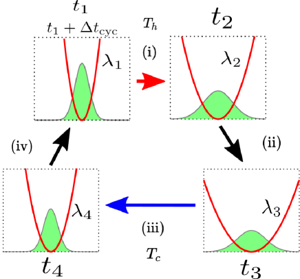
Figure 1: Schematic illustration of the Brownian Carnot cycle. In each box, the bottom horizontal line denotes the position coordinate $x$, and the boundary curve of the green filled area denotes the probability distribution of $x$. The red solid line corresponds to the harmonic potential with $\lambda_{i}$ ($i=1,2,3,4$). This cycle is composed of (i) the hot isothermal process, (ii) the finite-time adiabatic process, (iii) the cold isothermal process, and (iv) the finite-time adiabatic process.

We use the following protocol: (i) The hot isothermal process lasts for $t_{1}\leq t\leq t_{2}$. The temperature of the heat bath satisfies $T(t)=T_{h}$, and the stiffness $\lambda(t)$ changes from $\lambda_{1}$ to $\lambda_{2}$. (ii) The finite-time adiabatic process connecting the end of the hot isothermal process and the beginning of the cold one lasts for $t_{2}\leq t\leq t_{3}$. The temperature of the heat bath changes from $T_{h}$ to $T_{c}$, and the stiffness changes from $\lambda_{2}$ to $\lambda_{3}$. (iii) The cold isothermal process lasts for $t_{3}\leq t\leq t_{4}$. The temperature of the heat bath satisfies $T(t)=T_{c}$, and the stiffness $\lambda(t)$ changes from $\lambda_{3}$ to $\lambda_{4}$. (iv) The finite-time adiabatic process connecting the end of the cold isothermal process and the beginning of the hot one lasts for $t_{4}\leq t\leq t_{1}+\Delta t_{\rm cyc}$, where $\Delta t_{\rm cyc}$ is the cycle time. The temperature of the heat bath changes from $T_{c}$ to $T_{h}$, and the stiffness changes from $\lambda_{4}$ to $\lambda_{1}$.

In the above protocol, we assume that we can choose $\lambda_{1}$ and $\lambda_{2}$ arbitrarily and also assume that we choose the time taken for each process to be finite. When $\lambda_{2}$ is given, the initial value of $\tau_{x}$ of the finite-time adiabatic process (ii) is determined from Eq. (7). Then, since $\Delta t$ in this process is assumed to be finite, the condition of the finite-time adiabatic process in Eq. (46) should be satisfied because of the discussion in Sec. III. Applying Eq. (46) to the finite-time adiabatic process (ii), we impose the condition as

$$\frac{T_{c}^{2}}{\lambda_{3}}-\frac{T_{h}^{2}}{\lambda_{2}}=\alpha_{h\to c}\frac{\gamma}{\lambda_{2}^{2}},$$ (52)

where $\alpha_{h\to c}$ is a finite positive constant. Here, the indexes “$h\to c$” and “$c\to h$” denote the quantities in the finite-time adiabatic processes (ii) and (iv), respectively. When we give $\sigma_{x}(t)$ and $\Delta t$ in this process, we obtain the equation for $\alpha_{h\to c}$ and $\lambda_{3}$ from Eq. (47). By solving Eqs. (47) and (52) simultaneously, we can obtain $\alpha_{h\to c}$ and $\lambda_{3}$. In the finite-time adiabatic process (iv), the final value of $\tau_{x}$ is given since $\lambda_{1}$ is determined. Then, since $\Delta t$ in this process is assumed to be finite, the condition in Eq. (49) should be satisfied. Applying Eq. (49) to the finite-time adiabatic process (iv), we impose the condition as

$$\frac{T_{h}^{2}}{\lambda_{1}}-\frac{T_{c}^{2}}{\lambda_{4}}=\alpha_{c\to h}^{\prime}\frac{\gamma}{\lambda_{1}^{2}},$$ (53)

where $\alpha_{c\to h}^{\prime}$ is a finite positive constant. When we give $\sigma_{x}(t)$ and $\Delta t$ in this process, we can obtain $\lambda_{4}$ and $\alpha_{c\to h}^{\prime}$ by solving Eqs. (50) and (53) simultaneously. For convenience, we introduce the function $\phi(t)$ to describe the time evolution of the temperature $T(t)$ as

$$T(t)=\frac{T_{h}T_{c}}{T_{h}+\left(T_{c}-T_{h}\right)\phi(t)}.$$ (54)

In our Carnot cycle, since we assume that $T(t)$ is continuous, $\phi(t)$ should also be continuous, satisfying

$$\left\{\begin{array}[]{ll}\phi(t)=1&(t_{1}\leq t\leq t_{2})\\ 0\leq\phi(t)\leq 1&(t_{2}\leq t\leq t_{3})\\ \phi(t)=0&(t_{3}\leq t\leq t_{4})\\ 0\leq\phi(t)\leq 1&(t_{4}\leq t\leq t_{1}+\Delta t_{\rm cyc}).\end{array}\right.$$ (55)

IV.1 Construction of the Carnot cycle

In the hot isothermal process (i), the time taken for this process is given by

$$\Delta t_{h}\equiv t_{2}-t_{1}.$$ (56)

We choose $\Delta t_{h}$ as a finite value. When the entropy of the particle changes from $S_{1}$ to $S_{2}$ in this process, the entropy change $\Delta S_{h}$ in this process is given by

$$\Delta S_{h}\equiv S_{2}-S_{1}.$$ (57)

Substituting $T(t)=T_{h}$ into Eq. (II.1), the heat $Q_{h}$ flowing from the heat bath to the particle in this process is expressed by the entropy change of the particle $\Delta S_{h}$ and entropy production of the total system $\Sigma_{h}$ in this process as

$$Q_{h}=T_{h}\Delta S_{h}-T_{h}\Sigma_{h}.$$ (58)

Since the entropy production $\Sigma_{h}$ is nonnegative as seen from Eq. (II.1), we derive the inequality

$$T_{h}\Delta S_{h}\geq Q_{h}.$$ (59)

$Q_{h}>0$ should be satisfied since the heat should flow from the heat bath to the particle in the hot isothermal process in the Carnot cycle useful as a heat engine. Therefore, $T_{h}\Delta S_{h}$ as the upper bound of $Q_{h}$ in Eq. (59) has to be positive, and we obtain a necessary condition for the hot isothermal process:

$$S_{2}>S_{1}.$$ (60)

Since we consider the small relaxation-times regime, we can derive a condition for $\lambda_{1}$ and $\lambda_{2}$ from Eq. (60). From Eqs. (II) and (32), the entropy change in the hot isothermal process in this regime can be approximated by

$$\Delta S_{h}\simeq\frac{1}{2}\ln\left(\frac{\lambda_{1}}{\lambda_{2}}\right).$$ (61)

Because of $\Delta S_{h}>0$, $\lambda_{1}$ and $\lambda_{2}$ should satisfy

$$\lambda_{1}>\lambda_{2}.$$ (62)

Moreover, $\lambda_{1}/\lambda_{2}$ is finite because of the assumption above Eq. (27). Then, because of Eqs. (61) and (62), $\Delta S_{h}$ in the small relaxation-times regime is positively finite.

In the finite-time adiabatic process (ii), the entropy change of the particle $\Delta S_{h\to c}$ is equal to the entropy production of the total system $\Sigma_{h\to c}$ because of Eq. (40). When the entropy of the particle changes from $S_{2}$ to $S_{3}$, we obtain

$$\Delta S_{h\to c}\equiv S_{3}-S_{2}=\Sigma_{h\to c}.$$ (63)

From the nonnegatively of $\Sigma_{h\to c}$ in Eq. (II.1), the relation

$$S_{3}\geq S_{2}$$ (64)

should be satisfied. The time taken for this process is given by

$$\Delta t_{h\to c}\equiv t_{3}-t_{2}.$$ (65)

We choose $\Delta t_{h\to c}$ as a finite value.

In the isothermal process (iii), we can repeat the discussion similar to the isothermal process (i). In this process, the entropy of the particle changes from $S_{3}$ to $S_{4}$. Then, the time $\Delta t_{c}$ taken for this process, the entropy change $\Delta S_{c}$, and the heat $Q_{c}$ flowing from the heat bath to the particle in this process are given by

$$\Delta t_{c}\equiv t_{4}-t_{3},$$ (66)

$$\Delta S_{c}\equiv S_{4}-S_{3},$$ (67)

$$Q_{c}= T_{c}\Delta S_{c}-T_{c}\Sigma_{c},$$ (68)

where $\Sigma_{c}$ is the entropy production of the total system in this process. We choose $\Delta t_{c}$ as a finite value. Note that we cannot determine the sign of $\Delta S_{c}$ at this point by considering the sign of $Q_{c}$ unlike the case of the hot isothermal process (i). We will determine the sign of $\Delta S_{c}$ later by considering the sum of the entropy change of the particle during one cycle.

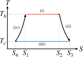
Figure 2: The entropy of the Brownian particle and temperature of the heat bath in our Carnot cycle with the finite-time adiabatic processes. From the restriction of the finite-time adiabatic processes, the entropy at the ends of the isothermal processes should satisfy $S_{2}\leq S_{3}$ and $S_{4}\leq S_{1}$.

In the finite-time adiabatic process (iv), the entropy change of the particle $\Delta S_{c\to h}$ is equal to the entropy production of the total system $\Sigma_{c\to h}$ because of Eq. (40). For the cycle to close, the entropy of the particle should change from $S_{4}$ to $S_{1}$, which leads to

$$\Delta S_{c\to h}\equiv S_{1}-S_{4}=\Sigma_{c\to h}.$$ (69)

Since the entropy production $\Sigma_{c\to h}$ is nonnegative, $S_{4}$ and $S_{1}$ should satisfy

$$S_{1}\geq S_{4}.$$ (70)

The time taken for this process is given by

$$\Delta t_{c\to h}\equiv(t_{1}+\Delta t_{\rm cyc})-t_{4}.$$ (71)

We choose $\Delta t_{c\to h}$ as a finite value.

After one cycle, the system returns to the initial state. Then, we obtain the trapezoidlike $T$-$S$ diagram of our cycle in Fig. 2 from Eqs. (60), (64), and (70). The sum of the entropy change of the particle satisfies

$$\Delta S_{h}+\Delta S_{h\to c}+\Delta S_{c}+\Delta S_{c\to h}=0.$$ (72)

Using Eqs. (63), (69), and (72), we obtain

$$\Delta S_{c}=-(\Delta S_{h}+\Sigma_{h\to c}+\Sigma_{c\to h}).$$ (73)

Using Eqs. (II) and (32), we find that the entropy change of the particle in the cold isothermal process in the small relaxation-times regime can be approximated by

$$\Delta S_{c}\simeq\frac{1}{2}\ln\left(\frac{\lambda_{3}}{\lambda_{4}}\right)<0,$$ (74)

where the last inequality comes from $\Delta S_{h}+\Sigma_{h\to c}+\Sigma_{c\to h}>0$ and Eq. (73). Then, we obtain

$$\lambda_{3}<\lambda_{4}.$$ (75)

From the first law of the thermodynamics, we derive the output work per cycle as

$$W= Q_{h}+Q_{c}$$

$$= T_{h}\Delta S_{h}+T_{c}\Delta S_{c}-T_{h}\Sigma_{h}-T_{c}\Sigma_{c}$$ (76)

$$= (T_{h}-T_{c})\Delta S_{h}-T_{h}\Sigma_{h}-T_{c}(\Sigma_{h\to c}+\Sigma_{c}+\Sigma_{c\to h}),$$

using Eqs. (58), (68), and (73). Since the entropy production of the total system in each process is nonnegative, the work $W$ has the upper bound $W_{0}$ as

$$W_{0}\equiv(T_{h}-T_{c})\Delta S_{h}\geq W.$$ (77)

Since $T_{h}-T_{c}$ and $\Delta S_{h}$ are finite, $W_{0}$ is also finite. When the entropy production in each process vanishes, we obtain $W=W_{0}$ from Eq. (IV.1). By using Eqs. (56), (65), (66), and (71), the time taken for each process satisfies

$$\Delta t_{\rm cyc}=\Delta t_{h}+\Delta t_{h\to c}+\Delta t_{c}+\Delta t_{c\to h}.$$ (78)

Since the time taken for each process is finite, $\Delta t_{\rm cyc}$ is finite. Using Eqs. (1), (59), and (77), we obtain the conditions for the efficiency $\eta$ and power $P$ of our cycle as

$$\eta\equiv \frac{W}{Q_{h}}\leq\frac{W_{0}}{T_{h}\Delta S_{h}}=\frac{(T_{h}-T_{c})\Delta S_{h}}{T_{h}\Delta S_{h}}=\eta_{\rm C},$$ (79)

$$P\equiv \frac{W}{\Delta t_{\rm cyc}}\leq\frac{W_{0}}{\Delta t_{\rm cyc}}=\frac{(T_{h}-T_{c})\Delta S_{h}}{\Delta t_{\rm cyc}}\equiv P_{0},$$ (80)

where $P_{0}$ is the power when $W=W_{0}$ is satisfied. When the entropy productions $\Sigma_{h}$, $\Sigma_{c}$, $\Sigma_{h\to c}$, and $\Sigma_{c\to h}$ vanish, $Q_{h}$ and $W$ approach $T_{h}\Delta S_{h}$ in Eq. (59) and $W_{0}$ in Eq. (77), respectively. Then, the efficiency approaches the Carnot efficiency $\eta_{\rm C}$ and the power approaches $P_{0}$.

V theoretical analysis

V.1 Trade-off relation

We show the trade-off relation between the efficiency $\eta$ and power $P$ in our cycle. From Eq. (II.1), we obtain the following inequality:

$$\dot{\Sigma}\geq \frac{\dot{Q}^{2}}{\gamma T\sigma_{v}},$$ (81)

or equivalently,

$$|\dot{Q}|\leq\sqrt{\gamma T\sigma_{v}\dot{\Sigma}}.$$ (82)

Since the finite-time adiabatic processes satisfy $\dot{Q}=0$, $Q_{h}$ can be written as

$$Q_{h}=\int^{t_{2}}_{t_{1}}dt\ \dot{Q}=\int^{t_{1}+\Delta t_{\rm cyc}}_{t_{1}}dt\ \phi(t)\dot{Q}(t),$$ (83)

where we used Eq. (55). Then, by using the Cauchy-Schwarz inequality, we derive the inequality for $Q_{h}$ as

$$Q_{h}^{2}= \left(\int^{t_{1}+\Delta t_{\rm cyc}}_{t_{1}}dt\ \phi\dot{Q}\right)^{2}$$

$$\leq \left(\int^{t_{1}+\Delta t_{\rm cyc}}_{t_{1}}dt\ \phi|\dot{Q}|\right)^{2}$$

$$\leq \left(\int^{t_{1}+\Delta t_{\rm cyc}}_{t_{1}}dt\ \phi\sqrt{\gamma T\sigma_{v}\dot{\Sigma}}\right)^{2}$$

$$\leq \Delta t_{\rm cyc}T_{c}^{2}\chi\Sigma_{\rm cyc},$$ (84)

using Eq. (82), where $\Sigma_{\rm cyc}$ is the entropy production of the total system per cycle and $\chi$ is defined as

$$\chi\equiv\frac{\gamma}{T_{c}^{2}\Delta t_{\rm cyc}}\int^{t_{1}+\Delta t_{\rm cyc}}_{t_{1}}dt\ \phi(t)^{2}T(t)\sigma_{v}(t).$$ (85)

Multiplying both sides of Eq. (V.1) by $W/(\Delta t_{\rm cyc}Q_{h}^{2})$, we derive the inequality for the power in Eq. (80) as

$$P\leq\frac{T_{c}^{2}\eta}{Q_{h}}\chi\Sigma_{\rm cyc},$$ (86)

using Eq. (79). Since the entropy change of the particle vanishes after one cycle, the entropy production of the total system per cycle is equal to that of the heat bath. Thus, the entropy production per cycle relates to the efficiency as

$$\Sigma_{\rm cyc}= -\frac{Q_{h}}{T_{h}}-\frac{Q_{c}}{T_{c}}$$

$$= \frac{Q_{h}}{T_{c}}(\eta_{\rm C}-\eta),$$ (87)

using Eqs. (1), (IV.1), and (79). From Eq. (V.1), it turns out that the efficiency becomes the Carnot efficiency when $\Sigma_{\rm cyc}$ vanishes. By using Eqs. (86) and (V.1), we can derive the trade-off relation between the efficiency and power:

$$P\leq\chi T_{c}\eta(\eta_{\rm C}-\eta).$$ (88)

This inequality is the same as Eq. (111) in Ref. [18], where we applied the method based on Ref. [25].

V.2 Compatibility of the Carnot efficiency and finite power

We show the compatibility of the Carnot efficiency and finite power in the vanishing limit of the relaxation times in our cycle. If the entropy productions of the total system in all the processes vanish, the entropy production per cycle vanishes. Then, we can achieve the Carnot efficiency because of Eq. (V.1), and the power also approaches a finite $P_{0}$ in Eq. (80). Thus, we evaluate the entropy production in each process in the small relaxation-times regime.

From Eq. (36), the entropy productions in the isothermal processes are given by

$$\Sigma_{h}\simeq \frac{1}{T_{h}}\int^{1}_{0}ds_{h}\frac{\frac{\tau_{v}}{\Delta t_{h}}\left(\frac{dQ}{ds_{h}}\right)^{2}+\frac{\tau_{x}}{\Delta t_{h}}\frac{T_{h}^{2}}{4}\left(\frac{d}{ds_{h}}\ln\frac{T_{h}}{\lambda}\right)^{2}}{T_{h}-\frac{\tau_{x}}{\Delta t_{h}}\frac{\tau_{v}}{\Delta t_{h}}\frac{T_{h}}{4}\left(\frac{d}{ds_{h}}\ln\frac{T_{h}}{\lambda}\right)^{2}},$$ (89)

$$\Sigma_{c}\simeq \frac{1}{T_{c}}\int^{1}_{0}ds_{c}\frac{\frac{\tau_{v}}{\Delta t_{c}}\left(\frac{dQ}{ds_{c}}\right)^{2}+\frac{\tau_{x}}{\Delta t_{c}}\frac{T_{c}^{2}}{4}\left(\frac{d}{ds_{c}}\ln\frac{T_{c}}{\lambda}\right)^{2}}{T_{c}-\frac{\tau_{x}}{\Delta t_{c}}\frac{\tau_{v}}{\Delta t_{c}}\frac{T_{c}}{4}\left(\frac{d}{ds_{c}}\ln\frac{T_{c}}{\lambda}\right)^{2}},$$ (90)

where $s_{h}$ and $s_{c}$ are the normalized times in the corresponding isothermal processes:

$$s_{h}\equiv\frac{t-t_{1}}{\Delta t_{h}},\quad s_{c}\equiv\frac{t-t_{3}}{\Delta t_{c}}.$$ (91)

In the isothermal processes, $\lambda$ is not constant because of Eqs. (62) and (75), while $T$ is constant. Then, from Eq. (34), we find that $dQ/ds_{h}$ in Eq. (89) and $dQ/ds_{c}$ in Eq. (90) are finite when $\lambda$ changes smoothly except when $\lambda$ takes extremal values. Thus, in the vanishing limit of the relaxation times, the integrand in Eqs. (89) and (90) vanishes, and $\Sigma_{h}$ and $\Sigma_{c}$ also vanish.

Since we choose $\Delta t_{h\to c}$ and $\Delta t_{c\to h}$ as finite values, $\alpha_{h\to c}$ and $\alpha^{\prime}_{c\to h}$ in Eqs. (52) and (53) are positively finite because of the discussion below Eq. (47). By applying Eqs. (48) and (51) to the present finite-time adiabatic processes (ii) and (iv), respectively, we derive the entropy productions of the total system in these processes as

$$\Sigma_{h\to c}\simeq \frac{1}{2}\ln\left(1+\frac{\alpha_{h\to c}\tau_{x}(t_{2})}{T_{h}^{2}}\right),$$ (92)

$$\Sigma_{c\to h}\simeq -\frac{1}{2}\ln\left(1-\frac{\alpha^{\prime}_{c\to h}\tau_{x}(t_{1})}{T_{h}^{2}}\right).$$ (93)

These entropy productions vanish in the vanishing limit of the relaxation times.

Note that there may exist an entropy production at the switchings between the isothermal and finite-time adiabatic processes. As shown in Appendix C, this entropy production is caused by the discontinuity of the time derivative of $T(t)$ and $\lambda(t)$ at the switchings, although we assume that $T(t)$ and $\lambda(t)$ are continuous. However, we can also show that this entropy production is negligible in the small relaxation-times regime.

Using Eqs. (89), (90), (92), and (93), we obtain the entropy production of the total system per cycle:

$$\Sigma_{\rm cyc}= \Sigma_{h}+\Sigma_{c}+\Sigma_{h\to c}+\Sigma_{c\to h}$$

$$\simeq \frac{1}{T_{h}}\int^{1}_{0}ds_{h}\frac{\frac{\tau_{v}}{\Delta t_{h}}\left(\frac{dQ}{ds_{h}}\right)^{2}+\frac{\tau_{x}}{\Delta t_{h}}\frac{T_{h}^{2}}{4}\left(\frac{d}{ds_{h}}\ln\frac{T_{h}}{\lambda}\right)^{2}}{T_{h}-\frac{\tau_{x}}{\Delta t_{h}}\frac{\tau_{v}}{\Delta t_{h}}\frac{T_{h}}{4}\left(\frac{d}{ds_{h}}\ln\frac{T_{h}}{\lambda}\right)^{2}}$$

$$+\frac{1}{T_{c}}\int^{1}_{0}ds_{c}\frac{\frac{\tau_{v}}{\Delta t_{c}}\left(\frac{dQ}{ds_{c}}\right)^{2}+\frac{\tau_{x}}{\Delta t_{c}}\frac{T_{c}^{2}}{4}\left(\frac{d}{ds_{c}}\ln\frac{T_{c}}{\lambda}\right)^{2}}{T_{c}-\frac{\tau_{x}}{\Delta t_{c}}\frac{\tau_{v}}{\Delta t_{c}}\frac{T_{c}}{4}\left(\frac{d}{ds_{c}}\ln\frac{T_{c}}{\lambda}\right)^{2}}$$

$$+\frac{1}{2}\ln\left(1+\frac{\alpha_{h\to c}\tau_{x}(t_{2})}{T_{h}^{2}}\right)$$

$$-\frac{1}{2}\ln\left(1-\frac{\alpha^{\prime}_{c\to h}\tau_{x}(t_{1})}{T_{h}^{2}}\right).$$ (94)

From the discussion below Eqs. (91) and (93), the entropy productions in all the processes vanish in the vanishing limit of the relaxation times, and $\Sigma_{\rm cyc}$ also vanishes in this limit. Then, the heat $Q_{h}$ in Eq. (58) and work $W$ in Eq. (IV.1) become $T_{h}\Delta S_{h}$ in Eq. (59) and $W_{0}$ in Eq. (77), respectively. Thus, the efficiency in Eq. (79) approaches the Carnot efficiency, and the power in Eq. (80) approaches $P_{0}$. Since $\Delta t_{\rm cyc}$ in Eq. (78) and $W_{0}$ are finite, $P_{0}$ is finite. Although this may seem to be inconsistent with the trade-off relation in Eq. (88), we below show that there is no inconsistency.

In the small relaxation-times regime, since $\sigma_{v}$ is approximated by Eq. (30), $\chi$ in Eq. (85) is approximated by

$$\chi\simeq \frac{1}{\tau_{v}\Delta t_{\rm cyc}T_{c}^{2}}\int^{t_{1}+\Delta t_{\rm cyc}}_{t_{1}}dt\ \phi^{2}T^{2}$$

$$= \frac{1}{\tau_{v}}\left(\frac{1}{T_{c}^{2}}\int^{1}_{0}ds_{\rm cyc}\ \phi^{2}T^{2}\right)$$

$$= \frac{C}{\tau_{v}},$$ (95)

where $s_{\rm cyc}\equiv(t-t_{1})/\Delta t_{\rm cyc}$, and $C$ is a constant defined as

$$C\equiv\frac{1}{T_{c}^{2}}\int^{1}_{0}ds_{\rm cyc}\ \phi^{2}T^{2}.$$ (96)

Since $T$ is finite and $\phi$ satisfies Eq. (55), $C$ is finite. From Eq. (V.2), $\chi$ turns out to diverge in the vanishing limit of the relaxation times.

Next, we consider the right-hand side of Eq. (86). In the small relaxation-times regime, $\chi\Sigma_{\rm cyc}$ in Eq. (86) is approximated by

$$\chi\Sigma_{\rm cyc}\simeq \frac{C}{T_{h}}\int^{1}_{0}ds_{h}\frac{\frac{1}{\Delta t_{h}}\left(\frac{dQ}{ds_{h}}\right)^{2}+\frac{\tau_{x}}{\tau_{v}\Delta t_{h}}\frac{T_{h}^{2}}{4}\left(\frac{d}{ds_{h}}\ln\frac{T_{h}}{\lambda}\right)^{2}}{T_{h}-\frac{\tau_{x}}{\Delta t_{h}}\frac{\tau_{v}}{\Delta t_{h}}\frac{T_{h}}{4}\left(\frac{d}{ds_{h}}\ln\frac{T_{h}}{\lambda}\right)^{2}}$$

$$+\frac{C}{T_{c}}\int^{1}_{0}ds_{c}\frac{\frac{1}{\Delta t_{c}}\left(\frac{dQ}{ds_{c}}\right)^{2}+\frac{\tau_{x}}{\tau_{v}\Delta t_{c}}\frac{T_{c}^{2}}{4}\left(\frac{d}{ds_{c}}\ln\frac{T_{c}}{\lambda}\right)^{2}}{T_{c}-\frac{\tau_{x}}{\Delta t_{c}}\frac{\tau_{v}}{\Delta t_{c}}\frac{T_{c}}{4}\left(\frac{d}{ds_{c}}\ln\frac{T_{c}}{\lambda}\right)^{2}}$$

$$+\frac{C}{2\tau_{v}}\ln\left(1+\frac{\alpha_{h\to c}\tau_{x}(t_{2})}{T_{h}^{2}}\right)$$

$$-\frac{C}{2\tau_{v}}\ln\left(1-\frac{\alpha^{\prime}_{c\to h}\tau_{x}(t_{1})}{T_{h}^{2}}\right)$$ (97)

from Eqs. (V.2) and (V.2). As shown below Eq. (91), $dQ/ds_{h}$ and $dQ/ds_{c}$ in the isothermal processes are finite except when $\lambda$ takes extremal values. Then, the first term of the numerator of the integrand in the first and second terms of Eq. (V.2) is positively finite even in the vanishing limit of the relaxation times since $\Delta t_{h}$ and $\Delta t_{c}$ are finite. Thus, the first and second terms in Eq. (V.2) do not vanish in the vanishing limit of the relaxation times, which means that $\chi\Sigma_{\rm cyc}$ does not vanish in this limit, while $\Sigma_{\rm cyc}$ vanishes and the efficiency approaches the Carnot efficiency because of Eq. (V.1). Therefore, the right-hand side of the trade-off relation in Eq. (86) does not vanish, which means that the finite power is allowed. In fact, the power also approaches the finite $P_{0}$ in this limit. Thus, the compatibility of the Carnot efficiency and finite power is achievable by taking the vanishing limit of the relaxation times in our Brownian Carnot cycle with arbitrary temperature difference.

VI Numerical simulation

We show numerical results of the compatibility of the Carnot efficiency and finite power in the vanishing limit of the relaxation times. In this simulation, we solved Eqs. (12)–(14) numerically by the fourth-order Runge-Kutta method. Our specific protocol in the isothermal processes is given by

$$T(t)= \ T_{h}\hskip 8.53581pt(t_{1}\leq t\leq t_{2}),$$

$$T(t)= \ T_{c}\hskip 8.53581pt(t_{3}\leq t\leq t_{4}),$$ (98)

$$\lambda_{h}(t)= \ \frac{T_{h}}{w_{1}\left[1+\left(\sqrt{w_{2}/w_{1}}-1\right)\frac{t-t_{1}}{\Delta t_{h}}\right]^{2}}\hskip 8.53581pt(t_{1}\leq t\leq t_{2}),$$

$$\lambda_{c}(t)= \ \frac{T_{c}}{w_{3}\left[1+\left(\sqrt{w_{4}/w_{3}}-1\right)\frac{t-t_{3}}{\Delta t_{c}}\right]^{2}}\hskip 5.69054pt(t_{3}\leq t\leq t_{4}),$$

where $\lambda_{h}(t)$ and $\lambda_{c}(t)$ are the time evolution of $\lambda(t)$ in the isothermal processes with temperatures $T_{h}$ and $T_{c}$, respectively, and $w_{j}$ ($j=1,2,3,4$) are positive parameters. This protocol is inspired by the optimal protocol in the overdamped Brownian Carnot cycle with the instantaneous adiabatic processes [27, 16] and used in our previous study [18]. From Eqs. (7) and (VI), we obtain

$$w_{j}=\frac{T(t_{j})}{\lambda_{j}}=\frac{T(t_{j})}{\gamma}\tau_{x}(t_{j}).$$ (99)

Note that, using Eqs. (30) and (99), we obtain

$$\sigma_{x}(t_{j})\simeq w_{j}$$ (100)

in the small relaxation-times regime. From Eqs. (62) and (99), $w_{2}/w_{1}>1$ should be satisfied. For all simulations, we fixed $w_{2}/w_{1}=2.0$, since we can choose $w_{1}$ and $w_{2}$ arbitrarily, corresponding to the assumption that we can choose $\lambda_{1}$ and $\lambda_{2}$ arbitrarily, as mentioned above Eq. (52). Note that $w_{2}/w_{1}$ should be finite since $\lambda_{1}/\lambda_{2}$ is finite as shown below Eq. (62). We also fixed $T_{c}=1.0$, $\Delta t_{h}=\Delta t_{c}=1.0$, and $\gamma=1.0$ and varied $w_{1}$, $m$, and the temperature difference $T_{h}-T_{c}$ (or equivalently, the temperature $T_{h}$). Note that Eqs. (99) and (100) satisfy the condition in Eq. (41).

We have to consider the finite-time adiabatic processes to determine $w_{3}$ and $w_{4}$. By using Eqs. (52), (53), and (99), we obtain

$$w_{3}=\frac{T_{h}}{T_{c}}w_{2}+\frac{\gamma\alpha_{h\to c}}{T_{h}^{2}T_{c}}w_{2}^{2},$$ (101)

$$w_{4}=\frac{T_{h}}{T_{c}}w_{1}-\frac{\gamma\alpha^{\prime}_{c\to h}}{T_{h}^{2}T_{c}}w_{1}^{2},$$ (102)

where $\alpha_{h\to c}$ and $\alpha_{c\to h}^{\prime}$ are constants. Below, we explain how to determine $w_{3}$, $w_{4}$, $\alpha_{h\to c}$, and $\alpha_{c\to h}^{\prime}$ from Eqs. (47), (50), (101), and (102) when $\Delta t_{h\to c}$ and $\Delta t_{c\to h}$ are given. First, we give $\sigma_{x}(t)$ in the finite-time adiabatic processes to obtain the protocol. From Eq. (100), we give $\sigma_{x,h\to c}(t)$ satisfying $\sigma_{xi,h\to c}=w_{2}$ and $\sigma_{xf,h\to c}=w_{3}$. Although $\sigma_{xi,h\to c}$ is given since we can give $w_{2}$, $\sigma_{xf,h\to c}$ is undetermined. Similarly, we give $\sigma_{x,c\to h}(t)$ satisfying $\sigma_{xi,c\to h}=w_{4}$ and $\sigma_{xf,c\to h}=w_{1}$, where $\sigma_{xf,c\to h}$ is given and $\sigma_{xi,c\to h}$ is undetermined. Moreover, we assume $\Delta t_{h\to c}=\Delta t_{c\to h}=1.0$. Using $\sigma_{x}(t)$, $\Delta t_{h\to c}$, and $\Delta t_{c\to h}$, we can obtain the equations for $w_{3}$, $w_{4}$, $\alpha_{h\to c}$, and $\alpha_{c\to h}^{\prime}$ from Eqs. (47) and (50) in our cycle. Then, solving those equations together with Eqs. (101) and (102), we can determine $w_{3}$, $w_{4}$, $\alpha_{h\to c}$, and $\alpha_{c\to h}^{\prime}$. Note that we can choose $\Delta t_{h\to c}$ and $\Delta t_{c\to h}$ arbitrarily as long as they are finite, although we set $\Delta t_{h\to c}=\Delta t_{c\to h}=1.0$ in our simulation for simplicity.

In the finite-time adiabatic processes, we give

$$\sigma_{x}(t)= \left\{\begin{array}[]{ll}w_{h\to c}(t)&(t_{2}\leq t\leq t_{3})\\ w_{c\to h}(t)&(t_{4}\leq t\leq t_{1}+\Delta t_{\rm cyc}),\end{array}\right.$$ (105)

$$w_{h\to c}(t)\equiv \ w_{2}+(w_{3}-w_{2})(t-t_{2})/\Delta t_{h\to c},$$ (106)

$$w_{c\to h}(t)\equiv \ w_{4}+(w_{1}-w_{4})(t-t_{4})/\Delta t_{c\to h}$$ (107)

to obtain the protocol. Then, from Eqs. (140) and (B) in Appendix B, we find that the protocol is obtained as

$$T_{h\to c}(t)= \left(1-\frac{w_{3}\frac{t-t_{2}}{\Delta t_{h\to c}}}{w_{h\to c}(t)}\right)T_{h}+\frac{w_{3}\frac{t-t_{2}}{\Delta t_{h\to c}}}{w_{h\to c}(t)}T_{c}$$

$$\hskip 99.58464pt(t_{2}\leq t\leq t_{3}),$$

$$T_{c\to h}(t)= \left(1-\frac{w_{1}\frac{t-t_{4}}{\Delta t_{c\to h}}}{w_{c\to h}(t)}\right)T_{c}+\frac{w_{1}\frac{t-t_{4}}{\Delta t_{c\to h}}}{w_{c\to h}(t)}T_{h}$$ (108)

$$\hskip 71.13188pt(t_{4}\leq t\leq t_{1}+\Delta t_{\rm cyc}),$$

$$\lambda_{h\to c}(t)= \frac{2T_{h\to c}(t)-\gamma\frac{\left(w_{3}-w_{2}\right)}{\Delta t_{h\to c}}}{2w_{h\to c}(t)}\quad(t_{2}\leq t\leq t_{3}),$$

$$\lambda_{c\to h}(t)= \frac{2T_{c\to h}(t)-\gamma\frac{\left(w_{1}-w_{4}\right)}{\Delta t_{c\to h}}}{2w_{c\to h}(t)}$$ (109)

$$\hskip 71.13188pt(t_{4}\leq t\leq t_{1}+\Delta t_{\rm cyc}).$$

Note that the approximate equality in Eq. (100) becomes equality only in the vanishing limit of the relaxation times. Although we derived the protocol in the adiabatic processes by regarding $\sigma_{x}(t_{j})$ as $w_{j}$ ($j=1,2,3,4$) in Eqs. (105)–(107), the equality in Eq. (100) is not satisfied exactly in the simulation. Thus, the time evolution of $\sigma_{x}(t)$ realized by solving Eqs. (12)–(14) with the protocol in Eqs. (VI) and (VI) is not exactly the same as the given $\sigma_{x}(t)$ in Eq. (105). However, their difference becomes small when the relaxation times are sufficiently small. Moreover, because the domains of $w_{h\to c}$ and $w_{c\to h}$ are $t_{2}\leq t\leq t_{3}$ and $t_{4}\leq t\leq t_{1}+\Delta t_{\rm cyc}$, respectively, they satisfy

$$0\leq\frac{w_{3}\frac{t-t_{2}}{\Delta t_{h\to c}}}{w_{h\to c}(t)},\ \frac{w_{1}\frac{t-t_{4}}{\Delta t_{c\to h}}}{w_{c\to h}(t)}\leq 1.$$ (110)

Thus, $T_{c}\leq T_{h\to c}(t),T_{c\to h}(t)\leq T_{h}$ is satisfied because of Eq. (VI). Then, $T_{h\to c}(t)$ and $T_{c\to h}(t)$ are finite at any time even in the vanishing limit of $w_{j}$ ($j=1,2,3,4$). By using Eq. (105), we can calculate the integral in Eqs. (47) and (50). Then, $\Delta t_{h\to c}$ and $\Delta t_{c\to h}$ in the small relaxation-times regime satisfy

$$\Delta t_{h\to c}\simeq \frac{T_{h}^{2}}{2\alpha_{h\to c}}\left(\frac{w_{3}}{w_{2}}-1\right)^{2},$$ (111)

$$\Delta t_{c\to h}\simeq \frac{T_{h}^{2}}{2\alpha_{c\to h}^{\prime}}\left(\frac{w_{4}}{w_{1}}-1\right)^{2}.$$ (112)

From Eqs. (101) and (102), we obtain

$$\frac{w_{3}}{w_{2}}=\frac{T_{h}}{T_{c}}+\frac{\gamma\alpha_{h\to c}}{T_{h}^{2}T_{c}}w_{2}\simeq\frac{T_{h}}{T_{c}},$$ (113)

$$\frac{w_{4}}{w_{1}}=\frac{T_{h}}{T_{c}}-\frac{\gamma\alpha^{\prime}_{c\to h}}{T_{h}^{2}T_{c}}w_{1}\simeq\frac{T_{h}}{T_{c}},$$ (114)

where the last approximate equalities hold because $w_{j}$ in Eq. (99) is sufficiently small in the small relaxation-times regime and $\alpha_{h\to c}$ and $\alpha^{\prime}_{c\to h}$ should be finite for any value of the relaxation times. Then, Eqs. (111) and (112) become

$$\Delta t_{h\to c}\simeq \frac{T_{h}^{2}}{2\alpha_{h\to c}}\left(\frac{T_{h}}{T_{c}}-1\right)^{2},$$ (115)

$$\Delta t_{c\to h}\simeq \frac{T_{h}^{2}}{2\alpha_{c\to h}^{\prime}}\left(\frac{T_{h}}{T_{c}}-1\right)^{2}.$$ (116)

Since we choose $\Delta t_{h\to c}=\Delta t_{c\to h}=1.0$, $\alpha_{h\to c}$ and $\alpha^{\prime}_{c\to h}$ are given by

$$\alpha_{h\to c}\simeq \frac{T_{h}^{2}}{2}\left(\frac{T_{h}}{T_{c}}-1\right)^{2},$$ (117)

$$\alpha_{c\to h}^{\prime}\simeq \frac{T_{h}^{2}}{2}\left(\frac{T_{h}}{T_{c}}-1\right)^{2}.$$ (118)

From Eqs. (101), (102), (117), and (118), we obtain $w_{3}$ and $w_{4}$.

By numerically calculating the integrals in Eqs. (22) and (23) from the solution to Eqs. (12)–(14), we obtained the heat $Q_{h}$ and $Q_{c}$ in Eqs. (58) and (68) and the work $W$ in Eq. (IV.1). Using the heat and work, we also calculated the efficiency $\eta=W/Q_{h}$ in Eq. (79) and power $P=W/\Delta t_{\rm cyc}$ in Eq. (80). In this simulation, we choose the initial condition as $\sigma_{x}(t_{1})=w_{1}$, $\sigma_{v}(t_{1})=T_{h}/m$, and $\sigma_{xv}(t_{1})=0$. Before starting to measure the thermodynamic quantities, we waited until the system settled down to a steady cycle. Therefore, our results are insensitive to the initial condition. When we consider the small relaxation-times regime in the present protocol, we should take the limit of $w_{1}\to 0$ and the limit of $m\to 0$ for the following reasons. In the limit of $w_{1}\to 0$, we can see that all $w_{j}$ vanish from $w_{2}/w_{1}=2.0$ and Eqs. (101) and (102). Then, $w_{h\to c}(t)$ in Eq. (106) and $w_{c\to h}(t)$ in Eq. (107) vanish at any time. Since $T(t)$ is finite at any time in the limit of $w_{1}\to 0$ as shown below Eq. (110), $\lambda(t)$ in Eqs. (VI) and (VI) diverges and the relaxation time of position $\tau_{x}(t)$ in Eq. (7) vanishes at any time. Moreover, in the limit of $m\to 0$, the relaxation time of velocity $\tau_{v}$ in Eq. (8) vanishes. Note that in the numerical simulations, we selected a time step smaller than the relaxation times. Specifically, we set the time step of the Runge-Kutta method as $\min(w_{1},m)\times 10^{-2}$ because of $\tau_{x}(t_{1})=\gamma w_{1}/T_{h}$ and $\tau_{v}=m/\gamma$.

We here confirm that the present protocol satisfies the assumption of finite $T(t^{\prime})/T(t)$ and $\lambda(t^{\prime})/\lambda(t)$, as mentioned above Eq. (27), where $t$ and $t^{\prime}$ are any times in a process. Since $T_{c}\leq T(t)\leq T_{h}$ is satisfied at any time, $T(t^{\prime})/T(t)$ is finite in all the processes. Moreover, from Eqs. (113) and (114) and the finite $w_{2}/w_{1}$, we find that $w_{3}/w_{1}$ and $w_{4}/w_{1}$ are also finite. Then, using Eqs. (VI), (106), (107), and (VI), we can confirm that $\lambda(t^{\prime})/\lambda(t)$ is finite in all the processes even in the vanishing limit of the relaxation times.

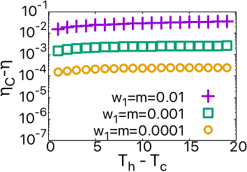
Figure 3: The difference between the Carnot efficiency and our efficiency measured with the protocol in Eqs. (VI), (VI), and (VI), when we vary the relaxation times $\tau_{x}(t_{1})$ and $\tau_{v}$, which are proportional to $w_{1}$ and $m$, respectively. In these simulations, we set $w_{1}=m=10^{-2}$ (purple plus), $w_{1}=m=10^{-3}$ (green square), and $w_{1}=m=10^{-4}$ (orange circle). The efficiency appears to approach the Carnot efficiency in the vanishing limit of $w_{1}$ (or $\tau_{x}$) and $m$ (or $\tau_{v}$).

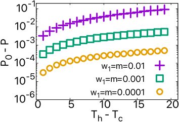
Figure 4: The power in Eq. (80) of our cycle, corresponding to Fig. 3. The power approaches $P_{0}$ in Eq. (120) in the vanishing limit of $w_{1}$ (or $\tau_{x}$) and $m$ (or $\tau_{v}$) for any temperature difference.

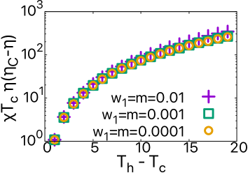
Figure 5: The right-hand side of Eq. (88) corresponding to Fig. 3. Although the efficiency approaches the Carnot efficiency in the limit of $w_{1},m\to 0$ ($\tau_{x},\tau_{v}\to 0$) in Fig. 3, $\chi T_{c}\eta(\eta_{\rm C}-\eta)$ remains almost unchanged. This means that $\chi$ diverges in this limit.

Figure 3 shows the difference between the Carnot efficiency and our efficiency measured with the protocol in Eqs. (VI), (VI), and (VI). In our previous study [18], the Carnot efficiency is achievable only in the small temperature-difference regime even when we take the vanishing limit of the relaxation times. In contrast to that, we can see that the efficiency approaches the Carnot efficiency in this limit even when the temperature difference is large.

Figure 4 shows the difference between $P_{0}$ in Eq. (80) and $P$ corresponding to Fig. 3. In the small relaxation-times regime, we obtain

$$\Delta S_{h}\simeq\frac{1}{2}\ln\left(\frac{w_{2}}{w_{1}}\right)=\frac{1}{2}\ln 2,$$ (119)

using $w_{2}/w_{1}=2.0$ and Eqs. (61) and (99). In the vanishing limit of the relaxation times, since the approximate equality in Eq. (30) becomes equality, the approximate equality in Eq. (119) also becomes equality. Then, we obtain $W_{0}=(T_{h}-T_{c})\ln 2/2$ because of Eq. (77). Since we use $\Delta t_{h}=\Delta t_{c}=\Delta t_{h\to c}=\Delta t_{c\to h}=1.0$, we have $\Delta t_{\rm cyc}=4.0$ in our simulation. Thus, we obtain

$$P_{0}=\frac{\ln 2}{8}(T_{h}-T_{c}),$$ (120)

from Eq. (80). From Fig. 4, we can see that the power approaches $P_{0}$ in the vanishing limit of the relaxation times for arbitrary temperature difference. Thus, the power turns out to be finite.

Figure 5 shows the upper bound of the power in Eq. (88). We can see that the upper bound of the power remains finite even when the efficiency approaches the Carnot efficiency as shown in Fig. 3. This means that $\chi$ in Eq. (85) diverges in the vanishing limit of the relaxation times, and also means that the finite power is allowed.

In Fig. 6, we compare the results of the numerical simulation with the theoretical analysis derived in Sec. V for the efficiency and power. To obtain the theoretical results in Fig. 6, we calculated the entropy productions in Eqs. (89), (90), (92), and (93). Note that we used Eq. (34) to calculate $\dot{Q}$ in Eqs. (89) and (90) from the time derivative of the protocol in Eq. (VI). Moreover, we set $\Delta S_{h}=\ln 2/2$ in the theoretical analysis as in the numerical simulation. Then, we derived the heat in the hot isothermal process and work from Eqs. (58) and (IV.1). Using the heat and work, we can obtain the efficiency in Eq. (79) and power in Eq. (80). The numerical simulation and theoretical analysis in Fig. 6 show good agreement. Thus, this result shows the validity of the theoretical analysis in Sec. V. From Figs. 3–5, we can see that the compatibility of the Carnot efficiency with finite power is achievable without breaking the trade-off relation.

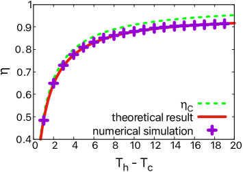
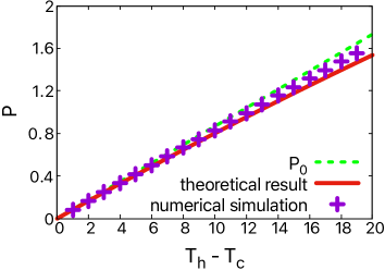
Figure 6: Efficiency (upper figure) and power (lower figure) derived from the numerical simulations in Figs. 3 and 4 (purple plus) and theoretical analysis (red solid line). We set $w_{1}=m=10^{-2}$. Although the relaxation times corresponding to these parameters are not very small among the parameters used in Fig. 3, the theoretical results and numerical simulations show a good agreement. We have confirmed a better agreement with smaller parameters (data not shown).

VII Summary

We studied the relaxation-times dependence of the efficiency and power in an underdamped Brownian Carnot cycle with the finite-time adiabatic processes [30, 31] and time-dependent harmonic potential. We showed that the compatibility of the Carnot efficiency and finite power is achievable in the vanishing limit of the relaxation times in our cycle. In our previous study [18], we showed that the compatibility of the Carnot efficiency and finite power is possible only in the small temperature-difference regime in the Brownian Carnot cycle with the instantaneous adiabatic processes. In this paper, we considered the finite-time adiabatic processes and represented the entropy production in terms of the relaxation times in the small relaxation-times regime. Then, the entropy production vanishes in the vanishing limit of the relaxation times. We constructed the Carnot cycle with the finite-time adiabatic processes in the small relaxation-times regime. By the theoretical analysis of our cycle, we derived the trade-off relation and showed that in the vanishing limit of the relaxation times, the entropy production per cycle vanishes, in other words, the efficiency approaches the Carnot efficiency. Then, we also showed that the finite power is achievable without breaking the trade-off relation in Eq. (88). Moreover, we confirmed that our theoretical analysis agrees with the results of our numerical simulation. We finally note that we can use other protocols satisfying the assumption above Eq. (27) and continuity at the switchings between the processes instead of the present protocol in our simulation.

APPENDIX A DERIVATION OF EQ. (30)

We show that the variables $\sigma_{x}$, $\sigma_{v}$, and $\sigma_{xv}$ behave like Eq. (30) in the small relaxation-times regime when the time-dependent temperature $T(t)$ and stiffness $\lambda(t)$ satisfy the assumption above Eq. (27). For the above purpose, we first show that the variables $\sigma_{x}$, $\sigma_{v}$, and $\sigma_{xv}$ relax toward Eq. (30) when the temperature $T$ and stiffness $\lambda$ are constant. After that, we consider the case that the temperature $T(t)$ and stiffness $\lambda(t)$ depend on time and show that these variables satisfy Eq. (30).

We assume that a thermodynamic process lasts for $t_{i}\leq t\leq t_{f}$ and we thus have $\Delta t=t_{f}-t_{i}$ in Eq. (18). The temperature $T$ and stiffness $\lambda$ are assumed to be constant. When we set $\sigma_{x}(t_{i})=\sigma_{x0}$, $\sigma_{v}(t_{i})=\sigma_{v0}$, and $\sigma_{xv}(t_{i})=\sigma_{xv0}$ as an initial condition, we can solve Eqs. (12)–(14) using the Laplace transform [28], and we can obtain $\sigma_{x}$ and $\sigma_{v}$ as follows:

$$\sigma_{x}(t)= \frac{T}{\lambda}+\frac{m}{\lambda}D_{1}e^{-\frac{\gamma}{m}(t-t_{i})}$$

$$+\frac{\left(\gamma+m\omega^{*}\right)^{2}}{4\lambda^{2}}D_{2}e^{-\left(\frac{\gamma}{m}-\omega^{*}\right)(t-t_{i})}$$

$$+\frac{\left(\gamma-m\omega^{*}\right)^{2}}{4\lambda^{2}}D_{3}e^{-\left(\frac{\gamma}{m}+\omega^{*}\right)(t-t_{i})},$$ (121)

$$\sigma_{v}(t)= \frac{T}{m}+D_{1}e^{-\frac{\gamma}{m}(t-t_{i})}+D_{2}e^{-\left(\frac{\gamma}{m}-\omega^{*}\right)(t-t_{i})}$$

$$+D_{3}e^{-\left(\frac{\gamma}{m}+\omega^{*}\right)(t-t_{i})},$$ (122)

where

$$\omega^{*}\equiv \frac{\gamma}{m}\sqrt{1-4\frac{m\lambda}{\gamma^{2}}},$$ (123)

$$D_{1}\equiv \frac{\lambda}{m{\omega^{*}}^{2}}\left(4\frac{T}{m}-2\sigma_{v0}-2\frac{\lambda}{m}\sigma_{x0}-2\frac{\gamma}{m}\sigma_{xv0}\right),$$ (124)

$$D_{2}\equiv -\frac{1}{2{\omega^{*}}^{2}}\left[\frac{\gamma T}{m^{2}}\left(\frac{\gamma}{m}-\omega^{*}\right)+\left(2\frac{\lambda}{m}-\frac{\gamma^{2}}{m^{2}}+\frac{\gamma}{m}\omega^{*}\right)\sigma_{v0}\right.$$

$$-2\frac{\lambda^{2}}{m^{2}}\sigma_{x0}\left.+2\frac{\lambda}{m}\left(-\frac{\gamma}{m}+\omega^{*}\right)\sigma_{xv0}\right],$$ (125)

$$D_{3}\equiv -\frac{1}{2{\omega^{*}}^{2}}\left[\frac{\gamma T}{m^{2}}\left(\frac{\gamma}{m}+\omega^{*}\right)+\left(2\frac{\lambda}{m}-\frac{\gamma^{2}}{m^{2}}-\frac{\gamma}{m}\omega^{*}\right)\sigma_{v0}\right.$$

$$-2\frac{\lambda^{2}}{m^{2}}\sigma_{x0}\left.+2\frac{\lambda}{m}\left(-\frac{\gamma}{m}-\omega^{*}\right)\sigma_{xv0}\right].$$ (126)

We can also derive $\sigma_{xv}$ using Eqs. (12) and (A). Note that since the exponential terms in Eqs. (A) and (A) vanish as $t\to\infty$, $\sigma_{x}$ and $\sigma_{v}$ relax to time-independent $T/\lambda$ and $T/m$, respectively. Using $\tau_{x}$ in Eq. (7) and $\tau_{v}$ in Eq. (8), we can rewrite Eq. (123) as

$$\omega^{*}=\frac{1}{\tau_{v}}\sqrt{1-4\frac{\tau_{v}}{\tau_{x}}}.$$ (127)

Then, the exponential functions in Eqs. (A) and (A) are represented by

$$e^{-\frac{\gamma}{m}(t-t_{i})} =e^{-\left(t-t_{i}\right)/\tau_{v}},$$ (128)

$$e^{-\left(\frac{\gamma}{m}-\omega^{*}\right)(t-t_{i})} =e^{-\left(1-\sqrt{1-4\frac{\tau_{v}}{\tau_{x}}}\right)\left(t-t_{i}\right)/\tau_{v}},$$ (129)

$$e^{-\left(\frac{\gamma}{m}+\omega^{*}\right)(t-t_{i})} =e^{-\left(1+\sqrt{1-4\frac{\tau_{v}}{\tau_{x}}}\right)\left(t-t_{i}\right)/\tau_{v}}.$$ (130)

By considering the magnitude relationship between $\tau_{x}$ and $\tau_{v}$, we show that the relaxation time of the system is evaluated as $\max(\tau_{x},\tau_{v})$. When $\tau_{x}\leq 4\tau_{v}$, $\omega^{*}$ in Eq. (127) becomes purely imaginary. Thus, we can consider that the exponential terms in Eqs. (A) and (A), which are expressed by Eqs. (128)–(130), are sufficiently smaller than the first terms of Eqs. (A) and (A) when

$$t-t_{i}\gg\tau_{v}$$ (131)

is satisfied. Therefore, we can regard the relaxation time of the system as $\tau_{v}$. On the other hand, the case of $\tau_{x}>4\tau_{v}$ is as follows. Since the exponential function of the second terms in Eqs. (A) and (A) is expressed by the relaxation times as in Eq. (128), it becomes sufficiently smaller than the first terms when Eq. (131) is satisfied. Moreover, because the fourth terms in Eqs. (A) and (A) are expressed by Eq. (130) and $1+\sqrt{1-4\tau_{v}/\tau_{x}}>1$, those terms are also sufficiently smaller than the first terms when Eq. (131) is satisfied. When $4\tau_{v}/\tau_{x}$ becomes small, however, $1-\sqrt{1-4\tau_{v}/\tau_{x}}$ in the exponent of Eq. (129), by which the third terms in Eqs. (A) and (A) are expressed, approaches 0 and we have to reconsider the case. When $\tau_{x}\gg\tau_{v}$, the exponent of Eq. (129) is approximated by

$$-\frac{1}{\tau_{v}}\left(1-\sqrt{1-4\frac{\tau_{v}}{\tau_{x}}}\right)\left(t-t_{i}\right)\simeq-\frac{2}{\tau_{x}}\left(t-t_{i}\right),$$ (132)

which makes Eq. (129) vanish when

$$t-t_{i}\gg\tau_{x}$$ (133)

is satisfied. Then, the third terms of Eqs. (A) and (A) are sufficiently smaller than the first terms. When $\tau_{x}\gg\tau_{v}$, the time for the third terms in Eqs. (A) and (A) to vanish is longer than the time for the second and fourth terms to vanish. Therefore, the relaxation time of the system is evaluated as $\tau_{x}$. In summary, the relaxation time of the system is represented by

$$\tau\equiv\max(\tau_{x},\tau_{v}).$$ (134)

Therefore, we can see that when $t-t_{i}\gg\tau$ is satisfied, $\sigma_{x}$ and $\sigma_{v}$ are approximated by

$$\sigma_{x}\simeq\frac{T}{\lambda},\quad\sigma_{v}\simeq\frac{T}{m}$$ (135)

from Eqs. (A) and (A). When $\sigma_{x}$ and $\sigma_{v}$ are changing toward Eq. (135), we consider that the system is in the relaxation. Moreover, when $t-t_{i}\gg\tau$ is satisfied, we use the phrase “after the relaxation.” Since the initial condition is included only in $D_{1}$, $D_{2}$, and $D_{3}$ in Eqs. (124)–(A), we find that the variables $\sigma_{x}$ and $\sigma_{v}$ relax to the values determined by $T$, $m$, and $\lambda$ even when we choose other initial conditions. In the limit of $\tau\to 0$, $\sigma_{x}$ and $\sigma_{v}$ satisfy Eq. (135) when $t-t_{i}>0$.

From Eq. (12), we can obtain $\sigma_{xv}$ by differentiating Eq. (A) with respect to time. Because $T$ and $\lambda$ are assumed to be constant, the time derivative of the first term in Eq. (A) vanishes. After the relaxation, we can see that the time derivative of the remaining terms in Eq. (A) also vanishes. Thus, $\sigma_{xv}$ vanishes after the relaxation.

Subsequently, we consider the thermodynamic process where the temperature $T(t)$ and stiffness $\lambda(t)$ depend on time. In the statement above Eq. (27), we assumed that $T(t)$ and $\lambda(t)$ vary smoothly and slowly. Then, in the small relaxation-times regime, we can expect that the fast relaxation dynamics rapidly vanishes and only the slow dynamics remains accompanying the change of $T(t)$ and $\lambda(t)$. Therefore, as the resulting approximate dynamics, we obtain the same expression as Eq. (135), by replacing the constant $T$ and $\lambda$ with the time-dependent variables $T(t)$ and $\lambda(t)$, respectively. Then, we obtain the time derivative of $\sigma_{x}(t)$ and $\sigma_{v}(t)$ after the relaxation in the process as

$$\dot{\sigma}_{x}(t)\simeq\frac{d}{dt}\left(\frac{T(t)}{\lambda(t)}\right)=\frac{T(t)}{\lambda(t)}\left(\frac{d}{dt}\ln\frac{T(t)}{\lambda(t)}\right),\ \dot{\sigma}_{v}(t)\simeq\frac{\dot{T}(t)}{m}.$$ (136)

From Eqs. (12) and (136), $\sigma_{xv}(t)$ becomes

$$\sigma_{xv}(t)=\frac{1}{2}\dot{\sigma}_{x}(t)\simeq\frac{1}{2}\frac{d}{dt}\left(\frac{T(t)}{\lambda(t)}\right)=\frac{T(t)}{2\lambda(t)}\left(\frac{d}{dt}\ln\frac{T(t)}{\lambda(t)}\right).$$ (137)

Therefore, we obtain the results in Eqs. (30) and (31) in the small relaxation-times regime. In Appendix C, we mention that we may need to reconsider these results at the switching between the processes.

APPENDIX B DERIVATION OF THE PROTOCOL IN THE FINITE-TIME ADIABATIC PROCESS

We derive the protocol of the finite-time adiabatic process by giving a finite $\Delta t$ and the time evolution of $\sigma_{x}(t)$. We assume that the finite-time adiabatic process lasts for $t_{i}\leq t\leq t_{f}$, and the temperature changes from $T_{i}$ to $T_{f}$. In the finite-time adiabatic process, we need to specify the time evolution of the five variables [$T(t)$ and $\lambda(t)$ in the protocol and $\sigma_{x}$, $\sigma_{v}$, and $\sigma_{xv}$ representing the state of the Brownian particle]. In the finite-time adiabatic process in Sec. III, however, there are only four equations in Eqs. (12)–(14) and (37). Therefore, we have insufficient number of the equations. However, we can obtain the closed equations if we give the time evolution of one of the five variables.

As we show below, we obtain the protocol by giving the time evolution of $\sigma_{x}(t)$. To determine the time evolution of $\sigma_{v}$, $\sigma_{xv}$, $T$, and $\lambda$, we solve Eqs. (12)–(14) and (37). From the given $\sigma_{x}$ and Eq. (12), we obtain $\sigma_{xv}$. Using Eqs. (12) and (37), we can rewrite Eqs. (13) and (14) as

$$\dot{T}= -\lambda\dot{\sigma}_{x},$$ (138)

$$m\ddot{\sigma}_{x}= 2T-2\lambda\sigma_{x}-\gamma\dot{\sigma}_{x}.$$ (139)

From Eq. (138), we obtain $\lambda(t)$ as

$$\lambda(t)=-\frac{\dot{T}(t)}{\dot{\sigma}_{x}(t)}.$$ (140)

Substituting this into Eq. (139), we derive the differential equation of $T$ as

$$\dot{T}+\left(\frac{d}{dt}\ln\sigma_{x}\right)T= \frac{1}{2}\left(\frac{d}{dt}\ln\sigma_{x}\right)\left(m\ddot{\sigma}_{x}+\gamma\dot{\sigma}_{x}\right).$$ (141)

By solving Eq. (141), we can derive the time evolution of $T(t)$ as

$$T(t)= \frac{1}{2\sigma_{x}(t)}\left(\gamma\int^{t}_{t_{i}}\dot{\sigma}_{x}(t)^{2}dt\right.$$

$$\left.+2T_{i}\sigma_{xi}+\frac{m}{2}\dot{\sigma}_{x}(t)^{2}-\frac{m}{2}\dot{\sigma}_{xi}{}^{2}\right),$$ (142)

using the initial condition $T(t_{i})=T_{i}$. Then, from Eq. (37), we obtain $\sigma_{v}$. Note that $\Delta\Phi$ in the finite-time adiabatic process satisfies

$$\Delta\Phi= \frac{\sigma_{xf}T_{f}}{m}-\frac{\sigma_{xi}T_{i}}{m}-\frac{1}{4}(\dot{\sigma}_{xf}{}^{2}-\dot{\sigma}_{xi}{}^{2})$$

$$= \frac{1}{2}\frac{\gamma}{m}\int^{t_{f}}_{t_{i}}\dot{\sigma}_{x}(t)^{2}dt,$$ (143)

where we used Eqs. (10), (12), (37), and (III). From Eqs. (B) and (B), we can confirm that $T(t)$ satisfies $T(t_{f})=T_{f}$. Substituting the given $\sigma_{x}(t)$ and $T$ in Eq. (B) into Eq. (140), we can obtain the time evolution of $\lambda(t)$.

APPENDIX C ENTROPY PRODUCTION AT THE SWITCHINGS

We show that the entropy production at the switchings between the isothermal and finite-time adiabatic processes can be neglected in the small relaxation-times regime. In Sec. IV, although we assumed that $T$ and $\lambda$ in our Carnot cycle are continuous at the switchings, we do not assume that the time derivatives of $T$ and $\lambda$ are continuous. If $\sigma_{xv}$ always satisfies Eq. (30) even in the vicinity of the switchings and the time derivative of $T$ and $\lambda$ are discontinuous at the switchings, $\sigma_{xv}$ becomes discontinuous. However, the variables $\sigma_{x}$, $\sigma_{v}$, and $\sigma_{xv}$ should be continuous because their time evolution is described by the differential equations in Eqs. (12)–(14). Thus, we may consider that the variables do not satisfy Eq. (30) just after the switchings and relax to Eq. (30). This means that there exists a relaxation just after the switchings.

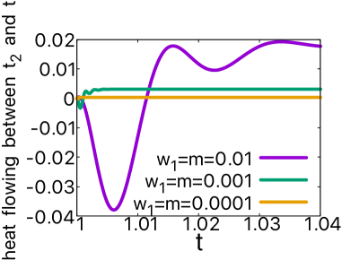
Figure 7: Heat flowing between $t_{2}$ and $t$ in the finite-time adiabatic process (ii) in Fig. 1. In this simulation, we used the protocol in Eqs. (VI), (VI), and (VI) in Sec. VI. We chose $T_{h}=10.0$, $T_{c}=1.0$, and the other parameters as in the numerical simulation in Sec. VI. We here set $t_{2}=1.0$. Thus, the finite-time adiabatic process (ii) lasts for $1.0\leq t\leq 2.0$. We find that although the relaxation after the switching at $t=t_{2}$ exists, the heat flowing in the relaxation becomes smaller when the relaxation times become smaller.

From Eq. (V.1), the entropy production per cycle should vanish to achieve the Carnot efficiency. Thus, the entropy production in the relaxation after the switchings may affect the efficiency. We evaluate the entropy production in the small relaxation-times regime and show that it can be neglected. Since the variables $\sigma_{x}$, $\sigma_{v}$, and $\sigma_{xv}$ may not satisfy Eqs. (30) and (31) in the relaxation, we cannot rewrite the entropy production rate by using the relaxation times as shown in Eq. (II.2). However, since the variables just before the switchings and after the relaxation satisfy Eqs. (30) and (31), we can evaluate the entropy change of the particle and heat flowing in the relaxation as shown below. Then, by using Eq. (II.1), we evaluate the entropy production.

Although we here focus on the switching from the hot isothermal process to the finite-time adiabatic process, corresponding to $t=t_{2}$ in Fig. 1, the similar discussion is available in the other switchings. At that switching, the temperature and stiffness satisfy $T=T_{h}$ and $\lambda=\lambda_{2}$, respectively. When $T$ and $\lambda$ vary smoothly and slowly, as in the statement above Eq. (27), we can expect that $T$ and $\lambda$ remain unchanged in the relaxation. Thus, the entropy change of the particle in this relaxation satisfies

$$\Delta S^{\rm rel}\simeq 0$$ (144)

in the small relaxation-times regime because of Eqs. (II) and (32), where the index “rel” means the quantity in this relaxation. Moreover, since $T$ and $\lambda$ are regarded as unchanged in the relaxation, we can see from Eq. (30) that each of $\sigma_{x}$ and $\sigma_{v}$ just before the relaxation takes the same value as that after the relaxation. Therefore, we can evaluate the heat $Q^{\rm rel}$ flowing in this relaxation in the small relaxation-times regime as

$$Q^{\rm rel}\simeq \frac{1}{2}m(\Delta\sigma_{v})^{\rm rel}+\frac{1}{2}\lambda_{2}(\Delta\sigma_{x})^{\rm rel}\simeq 0$$ (145)

from Eqs. (II.1) and (23). Figure 7 shows that the relaxation exists after the switching at $t=t_{2}$ in the finite-time adiabatic process (ii) in Fig. 1 with the protocol in Sec. VI. However, we can see that the heat flowing in the relaxation becomes smaller when the relaxation times become smaller. Thus, we can neglect $Q^{\rm rel}$ in Eq. (145) in the small relaxation-times regime. Since we can regard $T$ as $T_{h}$ in the relaxation, we derive the entropy production $\Sigma^{\rm rel}$ of the total system in this relaxation by using Eqs. (II.1), (144), and (145) as

$$\Sigma^{\rm rel}\simeq \Delta S^{\rm rel}-\frac{Q^{\rm rel}}{T_{h}}\simeq 0.$$ (146)

Thus, the entropy production $\Sigma^{\rm rel}$ can be neglected in the small relaxation-times regime.