Self-supervised Graph Learning for Occasional Group Recommendation

Abstract

As an important branch in Recommender System, occasional group recommendation has received more and more attention. In this scenario, each occasional group (cold-start group) has no or few historical interacted items. As each occasional group has extremely sparse interactions with items, traditional group recommendation methods can not learn high-quality group representations. The recent proposed Graph Neural Networks (GNNs), which incorporate the high-order neighbors of the target occasional group, can alleviate the above problem in some extent. However, these GNNs still can not explicitly strengthen the embedding quality of the high-order neighbors with few interactions. Motivated by the Self-supervised Learning technique, which is able to find the correlations within the data itself, we propose a self-supervised graph learning framework, which takes the user/item/group embedding reconstruction as the pretext task to enhance the embeddings of the cold-start users/items/groups. In order to explicitly enhance the high-order cold-start neighbors‘ embedding quality, we further introduce an embedding enhancer, which leverages the self-attention mechanism to improve the embedding quality for them. Comprehensive experiments show the advantages of our proposed framework than the state-of-the-art methods.

1 Introduction

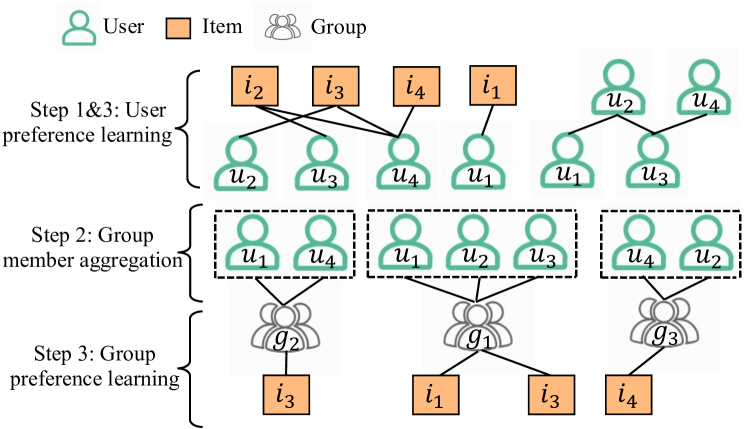
Figure 1: A running example for group recommendation.

As an important branch in Recommender System [48, 49, 50], occasional group recommendation has received more and more attention, and many social media platforms such as Meetup and Facebook aims to solve this problem [23, 24, 25, 26]. This task can be formulated as recommending items to occasional groups, where each occasional group has no or few historical interacted items. Since each occasional group has extremely sparse interactions with items, traditional group recommendation methods can not learn high-quality group representations.

To solve this problem, some early studies adopt heuristic pre-defined aggregation strategy such as average strategy [2], least misery strategy [5] and maximum satisfaction strategy [3] to aggregate the user preference to obtain the group preference. However, due to the fixed aggregation strategies, These methods are difficult to capture the complex dynamic process of group decision making, which results in unstable recommendation performance [32]. Further, Cao et al. [10] propose to assign each user an attention weight, which represents the influence of group member in deciding the group’s choice on the target item. However, when some users in the occasional group only interact with few items (a.k.a. cold-start users), the attention weight assigned for each user is diluted by these cold-start users, and thus results in biased group profile.

Recently, a few Graph Neural Networks (GNNs) based group recommendation methods are proposed [27, 12, 13, 16]. The core idea of these GNNs is to incorporate high-order neighbors as collaborative signals to strengthen the cold-start users’ embedding quality, and further enhance the embedding quality of the target group. As shown in Figure 1, the GNN model first conducts graph convolution multiple steps on the user-item and user-user interaction graphs to learn the preference of group members, and then performs average [16], summation and pooling [36] or attention mechanism [16] to aggregate the preferences of group members to obtain the group representation. Next, based on the aggregated embeddings of groups and users, the GNNs can estimate the probability that a group/user purchase an item. Finally, the recommendation-oriented loss (e.g., BPR loss [31]) is used to optimize the groups/users/items embeddings. Moreover, Zhang et al. [46] propose hypergraph convolution network (HHGR) with self-supervised node dropout strategy, which can model complex high-order interactions between groups and users. Through incorporating self-supervised signals, HHGR can alleviate the cold-start issue in some extent.

However, the above methods still suffer from the following challenges. First, the group representation not only depends on the group members’ preferences, but also relies on the group-level preferences towards items and collaborative group signals (the groups that share common users/items). Although some GNNs consider either group-level preferences [14] or collaborative group signals [16, 46] to form the group representation, they do not consider all these signals together. Second, the GNNs can not explicitly enhance the high-order cold-start neighbors’ embedding quality. For example in Figure 1, for the target group $g_{2}$, its group member $u_{1}$ and high-order neighbor $i_{1}$ only have few interactions. The embeddings of $u_{1}$ and $i_{1}$ are inaccurate, which will hurt the embedding quality of $g_{2}$ after performing graph convolution operation. Thus, how can we learn high-quality embeddings by GNNs for occasional group recommendation?

To this end, motivated by the self-supervised learning (SSL) technique [20, 19, 17], which aims to spontaneously find the supervised signals from the input data itself and can further benefit the downstream tasks [51, 52], we propose a self-supervised graph learning framework (${\rm SGG}$), which reconstructs the user/item group embedding with the backbone GNNs from multiple interaction graphs under the meta-learning setting [33]. ${\rm SGG}$ can explicitly improve the users’/items’/groups’ embedding quality. More concretely, first, we choose the groups/users/items that have enough interactions as the target groups/users/items. We treat the learned embeddings of these target groups/users/items as the ground-truth embeddings, since traditional recommendation algorithms can learn high-quality embeddings for them. Further, we mask a large proportion neighbors of the target groups/users/items to simulate the cold-start scenario, where the cold-start groups/users/items have few interactions. Based on the partially observed neighbors of the target groups/users/items, we perform graph convolution multiple steps to learn their ground-truth embeddings. More concretely, for each target group/user/item in their counterpart interaction graphs, we randomly sample $K$ first-order neighbors for them. Based on the sampled neighbors, we perform graph convolution operation multiple times in each interaction graph, and fuse the corresponding refined embeddings to predict the target embedding. Finally, we jointly optimize the reconstruction losses between the users’/items’/groups’ ground-truth embeddings and the predicted embeddings by the GNNs, which improves the convolution ability of the GNNs. Thus, the GNNs can obtain high-quality group representation that contains all the signals as presented in the first challenge.

Nevertheless, the above proposed embedding reconstruction task does not explicitly strengthen the high-order cold-start neighbors’ embedding quality for the target users/items/groups. To explicitly enhance the high-order cold-start neighbors’ embedding quality, we incorporate an embedding enhancer to learn high-quality node’s embeddings under the same meta-learning setting as mentioned before. The embedding enhancer is instantiated as the self-attention learner, which learns the cold-start nodes’ embeddings based on their masked first-order neighbors in the counterpart interaction graphs. We incorporate the meta embedding produced by the embedding enhancer into each graph convolution step to further strengthen the GNNs’ aggregation ability. The contributions are:

• We present a self-supervised graph learning framework for group recommendation. In this framework, we design the user/item/group embedding reconstruction task with GNNs under the meta-learning setting,

• We further introduce an embedding enhancer to strengthen the GNNs’ aggregation ability, which can improve the high-order cold-start neighbors’ embedding quality.

• Comprehensive experiments show the superiority of our proposed framework against the state-of-the-art methods.

2 Preliminary

2.1 Problem Definition

There are three sets of entities in the group recommendation scenario: $U=\ \{u_{1},\cdots,u_{|U|}\}$ denotes a user set, $I=\ \{i_{1},\cdots,i_{|I|}\}$ denotes an item set, and $G=\ \{g_{1},\cdots,g_{|G|}\}$ denotes a group set. There are three kinds of observed interaction graphs, i.e., group-item subgraph $\mathcal{G}_{GI}$, user-item subgraph $\mathcal{G}_{UI}$ and group-user subgraph $\mathcal{G}_{GU}$. Since the social connections of user-user and group-group are also important to depict the user and group profiles, we build two kinds of implicit interaction graphs based on $\mathcal{G}_{GI}$ and $\mathcal{G}_{UI}$, namely user-user subgraph $\mathcal{G}_{UU}$ and group-group subgraph $\mathcal{G}_{GG}$. In $\mathcal{G}_{UU}$, the two users are connected if they share with more than $c_{u}$ items. Similarly, in $\mathcal{G}_{GG}$, the two groups are connected if they share with more than $c_{g}$ items. Formally, notation $\mathcal{G}$ = $\{\mathcal{V},\mathcal{E}\}$ denotes the set of observed and implicit interaction graphs, i.e., $\mathcal{G}$ = $\mathcal{G}_{GI}\cup\mathcal{G}_{UI}\cup\mathcal{G}_{GU}\cup\mathcal{G}_{GG}\cup\mathcal{G}_{UU}$, where $\mathcal{E}$ is the edge set and $\mathcal{V}$ is the nodes set which contains $\{U,I,G\}$.

Definition 1. GNN-oriented Group Recommendation. Given the interaction graph $\mathcal{G}$, the goal is to train a GNN-based encoder $f$ that can recommend top-$k$ items for the target group $g$.

2.2 Base GNN for Group Recommendation

Although existing GNN-based group recommendation methods show their diversity in modelling group interactions with users and items [13, 12, 14, 16], we notice that they essentially share a general model structure. Based on this finding, we present a base GNN model, which consists of a representation learning module and a jointly training module. The representation learning module learns the representations of groups and users upon their counterpart interaction graphs, while the jointly training module optimizes the user/group preferences over items to compare the likelihood and the true user-item/group-item observations.

2.2.1 Representation Learning Module.

This module first learns the user representation upon the user-item and user-user subgraphs, and then learns the group representation upon the group-group, group-item and group-user subgraphs. Specifically, for each user $u$, we first sample his first-order neighbors on $\mathcal{G}_{UI}$ and $\mathcal{G}_{UU}$, and then perform graph convolution: $\textbf{h}_{u_{UI}}^{l}=\text{CONV}(\textbf{h}_{u_{UI}}^{l-1},\textbf{h}^{l}_{\mathcal{N}(u_{UI})})$, $\textbf{h}_{u_{UU}}^{l}=\text{CONV}(\textbf{h}_{u_{UU}}^{l-1},\textbf{h}^{l}_{\mathcal{N}(u_{UU})})$, where CONV can be instantiated into any GNN models, such as LightGCN [28] or GCN [41]. $\textbf{h}_{u_{UI}}^{l}$ and $\textbf{h}_{u_{UU}}^{l}$ denote the user embeddings calculated from $\mathcal{G}_{UI}$ and $\mathcal{G}_{UU}$ at the $l$-th graph convolution step, $\textbf{h}_{u_{UI}}^{0}$ and $\textbf{h}_{u_{UU}}^{0}$ are randomly initialized embeddings. $\textbf{h}^{l}_{\mathcal{N}(u_{UI})}$ and $\textbf{h}^{l}_{\mathcal{N}(u_{UU})}$ mean the averaged neighbor embeddings, where the neighbors are sampled from $\mathcal{G}_{UI}$ and $\mathcal{G}_{UU}$, respectively. After performing $L$-th convolution steps, we can obtain the refined user embeddings $\textbf{h}_{u_{UI}}^{L}$ and $\textbf{h}_{u_{UU}}^{L}$ from the counterpart subgraphs. Finally we conduct the soft-attention algorithm [22] to aggregate these embeddings to form the final user embedding $\textbf{h}_{u}^{L}$: $\textbf{h}_{u}^{L}=\sum_{c\in\{UI,UU\}}a_{c}\textbf{h}_{u_{c}}^{L}$, $a_{c}=\frac{{\rm exp}(\mathbf{W}_{c}\textbf{h}_{u_{c}}^{L})}{\sum_{c^{\prime}\in\{UI,UU\}}{\rm exp}(\mathbf{W}_{c^{\prime}}\textbf{h}_{u_{c^{\prime}}}^{L})}$, where $\{\mathbf{W}_{c}|c\in\{UI,UU\}\}$ are trainable parameters, $\{a_{c}|c\in\{UI,UU\}$ are the learned attention weight for each subgraph.

Then for each group $g$, we first sample its first-order neighbors from the $\mathcal{G}_{GI}$, $\mathcal{G}_{GU}$ and $\mathcal{G}_{GG}$, and perform graph convolution:

$$\textbf{h}_{g_{GI}}^{l} = \text{CONV}(\textbf{h}_{g_{GI}}^{l-1},\textbf{h}^{l}_{\mathcal{N}(g_{GI})}),$$ (1)

$$\textbf{h}_{g_{GU}}^{l} = \text{CONV}(\textbf{h}_{g_{GU}}^{l-1},\textbf{h}^{l}_{\mathcal{N}(g_{GU})}),$$

$$\textbf{h}_{g_{GG}}^{l} = \text{CONV}(\textbf{h}_{g_{GG}}^{l-1},\textbf{h}^{l}_{\mathcal{N}(g_{GG})}),$$

where $\textbf{h}_{g_{GI}}^{l}$, $\textbf{h}_{g_{GU}}^{l}$ and $\textbf{h}_{g_{GG}}^{l}$ denote the group embeddings calculated from $\mathcal{G}_{GI}$, $\mathcal{G}_{GU}$ and $\mathcal{G}_{GG}$ at the $l$-th graph convolution step, $\textbf{h}_{g_{GI}}^{0}$, $\textbf{h}_{g_{GU}}^{0}$ and $\textbf{h}_{g_{GG}}^{0}$ are randomly initialized embeddings. $\textbf{h}^{l}_{\mathcal{N}(g_{GI})}$, $\textbf{h}^{l}_{\mathcal{N}(g_{GU})}$ and $\textbf{h}^{l}_{\mathcal{N}(g_{GG})}$ mean the averaged neighbor embeddings, where the neighbors are sampled from $\mathcal{G}_{GI}$, $\mathcal{G}_{GU}$ and $\mathcal{G}_{GG}$, respectively. After performing $L$-th convolution steps, we can obtain the refined group embeddings $\textbf{h}_{g_{GI}}^{L}$, $\textbf{h}_{g_{GU}}^{L}$ and $\textbf{h}_{g_{GG}}^{L}$ from these three subgraphs. Same as existing works [14, 14, 16, 46], we further average the first-order neighbors in $\mathcal{G}_{GU}$ to obtain the aggregated group embedding $\textbf{h}_{g_{GU^{\prime}}}^{L}$,

$$\textbf{h}_{g_{GU^{\prime}}}^{L}=f_{agg}(\{\textbf{h}_{u_{GU}}^{L}|u\in\mathcal{N}(g_{GU})\}),$$ (2)

where $\textbf{h}_{u_{GU}}^{L}$ is obtained by performing graph convolution $L$ steps in $\mathcal{G}_{GU}$, $\mathcal{N}(g_{GU})$ denotes the first-order user set sampled from $\mathcal{G}_{GU}$, $f_{agg}$ is the aggregate function such as average [16], summation and pooling [36], or self-attention mechanism [9]. In our experiments, we find attention mechanism has the best performance. Finally, we use the soft-attention algorithm to aggregate the above embeddings to form the final group embedding $\textbf{h}_{g}^{L}$:

$$\textbf{h}_{g}^{L} = \sum_{c\in\{GI,GU,GU^{\prime},GG\}}a_{c}\textbf{h}_{g_{c}}^{L},$$ (3)

$$a_{c} = \frac{{\rm exp}(\mathbf{W}_{c}\textbf{h}_{g_{c}}^{L})}{\sum_{c^{\prime}\in\{GI,GU,GU^{\prime},GG\}}{\rm exp}(\mathbf{W}_{c^{\prime}}\textbf{h}_{g_{c^{\prime}}}^{L})},$$

where $\{\mathbf{W}_{c}|c\in\{GI,GU,GU^{\prime},GG\}\}$ are trainable parameters, $\{a_{c}\ |\ c\in\{GI,GU,\\ GU^{\prime},GG\}$ are the learned attention weights.

2.2.2 Jointly Training Module.

This module jointly optimizes the user preferences over items with the user-item loss $\mathcal{L}_{u}$ and the group preferences over items with the group-item loss $\mathcal{L}_{g}$, i.e., $\mathcal{L}_{main}=\mathcal{L}_{g}+\lambda\mathcal{L}_{u}$, where $\mathcal{L}_{main}$ is the final recommendation loss with a balancing hyper-parameter $\lambda$. Here, we use BPR loss [31] to calculate $\mathcal{L}_{u}$ and $\mathcal{L}_{g}$:

$$\mathcal{L}_{u} = \sum_{(u,i)\in\mathcal{E}_{UI},(u,j)\notin\mathcal{E}_{UI}}-\ln\sigma(y(u,i)-y(u,j)),$$ (4)

$$\mathcal{L}_{g} = \sum_{(g,i)\in\mathcal{E}_{GI},(g,j)\notin\mathcal{E}_{GI}}-\ln\sigma(y(g,i)-y(g,j)),$$

where $\sigma$ is the activation function, $y(u,i)={\textbf{h}_{u}^{L}}^{\mathrm{T}}\textbf{h}_{i}^{L}$, $y(g,i)={\textbf{h}_{g}^{L}}^{\mathrm{T}}\textbf{h}_{i}^{L}$, $\mathcal{E}_{UI}$ and $\mathcal{E}_{GI}$ represent the edges in $\mathcal{G}_{UI}$ and $\mathcal{G}_{GI}$.

Although the above presented GNNs can address the occasional groups through incorporating high-order collaborative signals, they still can not deal with the groups/users/items with few interactions, and thus can not learn high-quality embeddings for them.

3 The proposed model

We propose a self-supervised graph learning framework for group recommendation (${\rm SGG}$). We first describe the process of embedding reconstruction with GNN, and then detail an embedding enhancer which is incorporated into the backbone GNN model to further enhance the embedding quality. Finally, we present how ${\rm SGG}$ is trained and analyze its time complexity. The overall framework of ${\rm SGG}$ is shown in Figure 2.

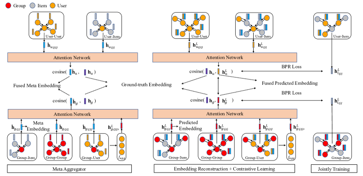
Figure 2: The overall framework of SGG. SGG contains a self-attention based embedding enhancer, which incorporates the generated meta embedding at each step of the original GNN convolution process.

3.1 Embedding Reconstruction with GNN

We propose embedding reconstruction with GNN, which jointly reconstructs the groups/users/items embeddings from multiple subgraphs under the meta-learning setting. Here we take the group embedding reconstruction as an example. Notably, the user/item embedding reconstruction process is similar to the group embedding reconstruction process. Specifically, first, we need the groups with abundant interactions as the target groups, and use any recommendation model such as AGREE [10] or LightGCN [28] to learn the embeddings of the target groups as the ground-truth embeddings. Then we mask a large proportion neighbors of the target group to simulate the occasional group. Based on the remained neighbors, we repeat the graph convolution operation multiple times to learn the ground-truth embeddings. Formally, for each target group $g$, we use notation $\textbf{h}_{g}$ to represent its ground-truth embedding. To mimic the occasional group, in each training episode, for each target group, we randomly sample $K$ items, $K$ users and $K$ groups from the corresponding group-item subgraph $\mathcal{G}_{GI}$, group-user subgraph $\mathcal{G}_{GU}$ and group-group subgraph $\mathcal{G}_{GG}$. We sample neighbors $L$ steps for each subgraph, i.e., for each target group, in each subgraph, we sample from its first-order neighbors to its $L$-order neighbors. After the sampling process is finished, for each target group, and for each subgraph, we can obtain at most $K^{l}(1\leq l\leq L)$ $l$-order neighbors. Next we use Eq. (1) to conduct the graph convolution operation $L$ steps from scratch to obtain the refined group embeddings $\textbf{h}_{g_{GI}}^{L}$, $\textbf{h}_{g_{GU}}^{L}$ and $\textbf{h}_{g_{GG}}^{L}$, use Eq. (2) to obtain the aggregated group embedding $\textbf{h}_{g_{GU^{\prime}}}^{L}$, and use Eq. (3) to obtain the fused group embedding $\textbf{h}_{g}^{L}$. Finally, following [35, 17], we measure the cosine similarity between $\textbf{h}_{g}$ and $\textbf{h}_{g}^{L}$, since the cosine similarity is a popularity indicator for the semantic similarity between embeddings:

$$\mathcal{L}_{R_{g}}:\mathop{\arg\max}_{\Theta_{f}}\sum_{g}{\rm cos}(\textbf{h}_{g}^{L},\textbf{h}_{g}),$$ (5)

where $\Theta_{f}$ is the parameters of the GNN model $f$. Similarly, we reconstruct the user embedding based on $\mathcal{G}_{UI}$ and $\mathcal{G}_{UU}$ with loss $\mathcal{L}_{R_{u}}$, and reconstruct the item embedding based on $\mathcal{G}_{UI}$ with loss $\mathcal{L}_{R_{i}}$. In practice, we jointly optimize group/user/item embedding reconstruction tasks with loss $\mathcal{L}_{R}$:

$$\mathcal{L}_{R}=\mathcal{L}_{R_{g}}+\mathcal{L}_{R_{u}}+\mathcal{L}_{R_{i}}.$$ (6)

Notably, the above proposed embedding reconstruction task is trained under the meta-learning setting, which enables the GNNs rapidly being adapted to new occasional groups. After we trained the model, when it comes to a new occasional group, given its first- and high-order neighbors, the pre-trained GNNs can generate a more accurate embedding for it. However, the above proposed embedding reconstruction task does not explicitly strengthen the high-order cold-start neighbors’ embedding quality. For example, if the high-order cold-start neighbors’ embeddings are biased, they will affect the embeddings of the target group when performing graph convolution. As shown in Fig. 1, for the target group $g_{2}$, its group member $u_{1}$ and high-order neighbor $i_{1}$ only have few interactions. The embeddings of $u_{1}$ and $i_{1}$ are inaccurate, which will hurt the embedding quality of $g_{2}$ after performing graph convolution operation. To solve this problem, we further incorporate an embedding enhancer into the above embedding reconstruction GNN model.

3.2 Embedding Enhancer

To explicitly strengthen the embedding quality of the high-order cold-start neighbors, we propose the embedding enhancer, which also learns the ground-truth group/user/item embedding, but only based on the first-order neighbors of the target group/user/item sampled from the counterpart graphs. Specifically, before we train the above embedding reconstruction task with GNNs, we train the embedding enhancer $f_{meta}$ under the same meta-learning setting as proposed in Section 3.1. Once the embedding enhancer $f_{meta}$ is trained, we combine the enhanced group/user/item embedding produced by $f_{mata}$ with the original group/user/item embedding at each graph convolution step to improve the cold-start neighbors’ embeddings. Notably, the GNN model is to strengthen the cold-start groups’/users’/items’ embedding quality, while the embedding enhancer is to improve the high-order cold-start neighbors’ embedding quality.

Here we take group embedding as an example. The embedding enhancer tackles the user/item embedding is similar to the group embedding. Specifically, the embedding enhancer $f_{meta}$ is instantiated as a self-attention learner [9]. For each group $g$, the embedding enhancer accepts the randomly initialized first-order embeddings $\{\textbf{h}_{i_{GI_{1}}}^{0},\cdots,\textbf{h}_{i_{GI_{K}}}^{0}\}$, $\{\textbf{h}_{u_{GU_{1}}}^{0},\cdots,\textbf{h}_{u_{GU_{K}}}^{0}\}$ and $\{\textbf{h}_{g_{GG_{1}}}^{0},\cdots,\textbf{h}_{g_{GG_{K}}}^{0}\}$ from the corresponding subgraphs $\mathcal{G}_{GI}$, $\mathcal{G}_{GU}$ and $\mathcal{G}_{GG}$ as input, outputs the smoothed embeddings $\{\textbf{h}_{i_{GI_{1}}},\cdots,\textbf{h}_{i_{GI_{K}}}\}$, $\{\textbf{h}_{u_{GU_{1}}},\cdots,\textbf{h}_{u_{GU_{K}}}\}$ and $\{\textbf{h}_{g_{GG_{1}}},\cdots,\textbf{h}_{g_{GG_{K}}}\}$, and use the average function to obtain the meta embedding $\hat{\textbf{h}}_{g_{GI}}$, $\hat{\textbf{h}}_{g_{GU}}$, $\hat{\textbf{h}}_{g_{GG}}$. The process is:

$$\{\textbf{h}_{i_{GI_{1}}},\cdots,\textbf{h}_{i_{GI_{K}}}\} \leftarrow \text{SELF\_ATTENTION}(\{\textbf{h}_{i_{GI_{1}}}^{0},\cdots,\textbf{h}_{i_{GI_{K}}}^{0}\}),$$

$$\hat{\textbf{h}}_{g_{GI}} = \text{AVERAGE}(\{\textbf{h}_{i_{GI_{1}}},\cdots,\textbf{h}_{i_{GI_{K}}}\}),$$ (7)

where the embedding $\hat{\textbf{h}}_{g_{GU}}$ and $\hat{\textbf{h}}_{g_{GG}}$ can be obtained in the same way. Furthermore, the aggregated group embedding $\textbf{h}_{g_{GU^{\prime}}}^{L}$ in Eq. (2) is also considered to reconstruct the group embedding. Finally, $f_{meta}$ fuses these embeddings using Eq. (3) to obtain another meta embedding $\hat{\textbf{h}}_{g}$.

The advantage of the self-attention learner is to pull the similar nodes more closer, while pushing away dissimilar nodes. Thus, the self-attention technique can capture the major group/user/item preference from its neighbors. Same with Section 3.1, the same cosine similarity (i.e., Eq.(5)) is used between $\hat{\textbf{h}}_{g}$ and $\textbf{h}_{g}$ to measure their similarity. Once the embedding enhancer $f_{meta}$ is trained, we incorporate the meta embedding $\hat{\textbf{h}}_{g_{GI}}$, $\hat{\textbf{h}}_{g_{GU}}$ and $\hat{\textbf{h}}_{g_{GG}}$ produced by the embedding enhancer into the GNN model at each graph convolution step (i.e., we add the meta embedding into Eq. (1)):

$$\textbf{h}_{g_{GI}}^{l} = \text{CONV}(\hat{\textbf{h}}_{g_{GI}},\textbf{h}_{g_{GI}}^{l-1},\textbf{h}^{l}_{\mathcal{N}(g_{GI})}),$$ (8)

$$\textbf{h}_{g_{GU}}^{l} = \text{CONV}(\hat{\textbf{h}}_{g_{GU}},\textbf{h}_{g_{GU}}^{l-1},\textbf{h}^{l}_{\mathcal{N}(g_{GU})}),$$

$$\textbf{h}_{g_{GG}}^{l} = \text{CONV}(\hat{\textbf{h}}_{g_{GG}},\textbf{h}_{g_{GG}}^{l-1},\textbf{h}^{l}_{\mathcal{N}(g_{GG})}).$$

For a target group $g$, we repeat Eq. (8) $L$ steps to obtain the embeddings $\textbf{h}_{g_{GI}}^{L}$, $\textbf{h}_{g_{GU}}^{L}$, $\textbf{h}_{g_{GG}}^{L}$. Then, we use Eq. (2) to obtain the aggregated group embedding $\textbf{h}_{g_{GU^{\prime}}}^{L}$, and use Eq. (3) to obtain the final group embedding $\textbf{h}_{g}^{L}$. Finally, we also use cosine similarity (i.e., Eq. (5)) to optimize the model parameters including the GNNs’ parameters $\Theta_{f}$ and the embedding enhancer’s parameters $\Theta_{f_{meta}}$. Similarly, the embedding enhancer $f_{meta}$ can obtain the enhanced user embedding on $\mathcal{G}_{UI}$ and $\mathcal{G}_{UU}$, and the enhanced item embedding on $\mathcal{G}_{UI}$.

3.3 Model Training

We conduct multi-task learning paradigm [45] to optimize the model parameters, i.e., we jointly train the recommendation objective function (cf. Eq. (4)) and the designed SSL objective function (cf. Eq. (6)):

$$\mathcal{L}=\mathcal{L}_{main}+\lambda_{1}\mathcal{L}_{R}+\lambda_{2}||\Theta||^{2}_{2},$$ (9)

where $\Theta$ = $\{\Theta_{f},\Theta_{f_{meta}}\}$ is the model parameters, $\lambda_{1}$ and $\lambda_{2}$ are hyperparameters. We also consider another training paradigm [17], i.e., pre-train the GNNs on $\mathcal{L}_{R}$ and fine-tune the GNNs on $\mathcal{L}_{main}$. We detail the recommendation performance of the two training paradigms in Section 4.4.3.

Table 1: The time complexity analysis between GNN and SGG.

Component	GNN	${\rm SGG}$
Adjacency Matrix	$\mathcal{O}(2|\mathcal{E}|)$	$\mathcal{O}(10|\hat{\mathcal{E}|}s+2|\mathcal{E}|)$
Graph Convolution	$\mathcal{O}(2|\mathcal{E}|Lds\frac{|\mathcal{E}|}{B})$	$\mathcal{O}(2(|\mathcal{E}|+5|\hat{\mathcal{E}}|)Lds\frac{|\mathcal{E}|}{B})$
BPR Objective Function	$\mathcal{O}(2|\mathcal{E}|ds)$	$\mathcal{O}(2|\mathcal{E}|ds)$
Self-supervised Objective Function	-	$\mathcal{O}(20|\hat{\mathcal{E}}|Lds)$

3.4 Time and Space Complexity Analysis

We present the time and space complexity of ${\rm SGG}$, and compare its time and space complexity with the backbone GNN model. Same as LightGCN [28], we implement ${\rm SGG}$ as the matrix form. Suppose the number of edges in the interaction graph $\mathcal{G}$ is $|\mathcal{E}|$. The number of edges in the masked interaction graph $\hat{\mathcal{G}}$ is $|\hat{\mathcal{E}}|$. Since we mask a large proportion neighbors for each node in $\mathcal{G}$ to simulate the cold-start scenario, the size of masked edge set is far less than the original edge set, i.e., $|\hat{\mathcal{E}}|\ll|\mathcal{E}|$. Let $s$ denote the number of epochs, $d$ denote the embedding size and $L$ denote the GCN convolution layers. Since ${\rm SGG}$ introduces meta embedding to enhance the aggregation ability, the space complexity of ${\rm SGG}$ is twice than that of the vanilla GNN model. The time complexity comes from four parts, namely adjacency matrix normalization, graph convolution operation, recommendation objective function and self-supervised objective function. Since we do not change the GNN’s model structure and GNN’s inference process, the time complexity of ${\rm SGG}$ in the graph convolution operation and recommendation objective function is the same as the vanilla GNN model. We present the main differences between the vanilla GNN and ${\rm SGG}$ models as follows:

• Adjacency matrix normalization. In each training epoch, generating the target group embedding needs five corresponding subgraphs. Suppose the non-zero elements in the adjacency matrices of the full training graph and the five subgraphs are $2|\mathcal{E}|$, $2|\hat{\mathcal{E}}_{UU}|$, $2|\hat{\mathcal{E}}_{UI}|$, $2|\hat{\mathcal{E}}_{GG}|$, $2|\hat{\mathcal{E}}_{GU}|$ and $2|\hat{\mathcal{E}}_{GI}|$, respectively. Thus, the total complexity of adjacency matrix normalization is $\mathcal{O}((2|\hat{\mathcal{E}}_{UU}|+2|\hat{\mathcal{E}}_{UI}|+2|\hat{\mathcal{E}}_{GG}|+2|\hat{\mathcal{E}}_{GU}|+2|\hat{\mathcal{E}}_{GI}|)s+2|\mathcal{E}|)\approx 10|\hat{\mathcal{E}}|s+2|\mathcal{E}|$. 

• Self-supervised objective function. We evaluate the self-supervised tasks upon the masked subgraphs. For the user or item embedding reconstruction task, the time complexity is $\mathcal{O}(2d*(2|\hat{\mathcal{E}}_{UU}|+2|\hat{\mathcal{E}}_{UI}|)*s*L)\approx 8|\hat{\mathcal{E}}|Lds$. For the group embedding reconstruction task, the time complexity is $\mathcal{O}(2d*(2|\hat{\mathcal{E}}_{GG}|+2|\hat{\mathcal{E}}_{GU}|+2|\hat{\mathcal{E}}_{GI}|)*s*L)\approx 12|\hat{\mathcal{E}}|Lds$, where $2d$ represents the concatenated embedding size, as we incorporate the meta embedding to the graph convolution process. Thus the total time complexity of self-supervised loss is $8|\hat{\mathcal{E}}|Lds+12|\hat{\mathcal{E}}|Lds=20|\hat{\mathcal{E}}|Lds$.

We summarize the time complexity between the vanilla GNNs and ${\rm SGG}$ in Table 1, from which we observe that the time complexity of ${\rm SGG}$ is in the same magnitude with the vanilla GNNs, which is totally acceptable, since the increased time complexity of ${\rm SGG}$ is only from the self-supervised loss. The details are shown in Section 4.4.1.

4 Experiments

We conduct comprehensive experiments to answer the following questions:

• Q1: Can ${\rm SGG}$ have better performance than the other baselines?

• Q2: Can the proposed self-supervised task benefit the occasion group recommendation task?

• Q3: How does ${\rm SGG}$ perform in different settings?

4.1 Experimental Settings

4.1.1 Datasets.

We select three public recommendation datasets, i.e., Weeplaces [27], CAMRa2011 [10] and Douban [1] to evaluate the performance of ${\rm SGG}$. Table 1 shows the statistics of these three datasets.

Table 2: Statistics of the Datasets.

	Weeplaces	CAMRa2011	Douban
Users	8,643	602	70,743
Items	25,081	7,710	60,028
Groups	22,733	290	109,538
U-I Interactions	1,358,458	116,314	3,422,266
G-I Interactions	180,229	145,068	164,153
U-I Sparsity	6.27%	2.51%	0.081%
G-I Sparsity	0.03%	6.49%	0.002%

4.1.2 Baselines.

We select the following baselines:

• MoSAN [6] adopts sub-attention mechanism to model the group-item interactions.

• AGREE [10] adopts attention mechanism for jointly modelling user-item and group-item interactions.

• SIGR [1] further incorporates social relationships of groups and users to model the attentive group and user representations.

• GroupIM [27] further regularizes group and user representations by maximizing the mutual information between the group and its members.

• GAME [14] performs graph convolution only based on the first-order neighbors from the group-group, group-user and group-item graphs for group recommendation.

• GCMC [40] uses the classical GCN [41] model to perform graph convolution, and learn the node embeddings.

• NGCF [42] adds second-order interactions upon the neural passing based GNN model [43].

• LightGCN [28] devises the light graph convolution upon NGCF.

• HHGR [46] designs coarse- and fine-grained node dropout strategies upon the hypergraph for group recommendation.

We discard potential baselines like Popularity [38], COM [8], and CrowdRec [39], since previous works [6, 10, 1, 27, 14] have validated the superiority over the compared ones. For the GNN model GCMC, NGCF and LightGCN, we extend it to address group recommendation as proposed in Section 2.2; Besides, notation GNN* denotes the corresponding proposed model ${\rm SGG}$. We further evaluate two variants of ${\rm SGG}$, named Basic-GNN and Meta-GNN, which are equipped with basic embedding reconstruction with GNNs (Section 3.1) and embedding enhancer (Section 3.2), respectively.

4.1.3 Training Settings.

We present the details of dataset segmentation, model training process and hyper-parameter settings.

Dataset Segmentation. We first select the groups with abundant interactions as the target groups in the meta-training set $D_{T}^{g}$ , and leave the rest groups in the meta-test set $D_{N}^{g}$, as we need more accurate embeddings of groups to evaluate the quality of the generated group embeddings. The splitting strategy of the users/items is the same with the groups. In order to avoid information leakage, we further select items with sufficient interactions from the group meta-training set $D_{T}^{g}$ and the user meta-training set $D_{T}^{u}$, and obtain the meta-training set $D_{T}^{i}$. For simplicity, we use $D_{T}$ and $D_{N}$ to denote these meta-training and meta-test sets. For each group/user in $D_{N}$, according to the interaction time with items, we further choose the former $c$% items into the training set $Train_{N}$, and leave the other items into the test set $Test_{N}$.

More concretely, for addressing the occasional groups, we split the dataset according to a predefined hyperparameter $n_{g}$. If a group interacts with more than $n_{g}$ items, we put it in $D_{T}$. Otherwise, we leave the group in $D_{N}$. We select $n_{g}$ as 10 for Weeplaces and Douban. Similarly, for the users/items with few interactions, we split the dataset according to $n_{u}$ ($n_{i}$). Both $n_{u}$ and $n_{i}$ is set as 10 for Weeplaces and Douban. In CAMRa2011, since the groups, users and items have abundant interactions, we randomly select 70% groups, users and items in $D_{T}$ and leave the rest in $D_{N}$. For each group and user in $D_{N}$, in order to simulate the real cold-start scenario, we only keep top 10 interacted items in chronological order. Similarly, for each item in $D_{N}$, we only keep its first 5 interacted groups/users.

Model Training Process. We train each of the baseline methods to obtain the ground-truth embeddings on $D_{T}$, since these methods can learn high-quality embeddings for the target nodes with enough interactions. For MoSAN, AGREE, SIGR, GroupIM and GAME, we directly fetch the trained embeddings as ground-truth embeddings; For the hypergraph GNN model HHGR and the general GNNs (i.e., LightGCN, NGCF and GCMC), we first fetch the embeddings at each layer and then concatenate them to obtain the final ground-truth embeddings. Take the group embedding as an example, $\textbf{h}_{g}$ = $\textbf{h}_{g}^{0}$ + $\cdots$+ $\textbf{h}_{g}^{L}$. User and item embeddings can be explained in the similar way.

The SSL tasks is trained on $D_{T}$, while the recommendation task is trained on $D_{T}$ and $Train_{N}$. Both the SSL and the recommendation tasks are evaluated in $Test_{N}$. We adopt Recall@$\mathcal{K}$ and NDCG@$\mathcal{K}$ as evaluation metric.

Hyper-parameter Settings. We use Xavier method [44] to initialize the parameters of all the models. We set the learning rate as 0.001 and the mini-batch size as 256. We tune $K$, $L$, $c\%$ within the ranges of {3, 4, 5, 6, 7, 8, 9, 10, 11, 12}, {1,2,3,4} and {0.1, 0.2, 0.3}, respectively. We tune $\lambda_{1}$ with the ranges of {0.01, 0.1, 0.5, 1.0, 1.2}, and empirically set $\lambda$ and $\lambda_{2}$ as 1 and 1e-6, respectively. We tune $c_{u}$ and $c_{g}$ with the ranges of {10, 20, 30}. By default, we set $L$ as 3, $K$ as 5, $c$% as 0.1, $\tau$ as 0.2, $c_{u}$ and $c_{g}$ as 20, and $\mathcal{K}$ as 20.

Table 3: Overall performance with sparse rate $c\%$=0.1, layer size $L$=3 and neighbor size $K$=5.

Methods	Weeplaces		CAMRa2011		Douban
	Recall	NDCG	Recall	NDCG	Recall	NDCG
${\rm MoSAN}$	0.0223	0.0208	0.0214	0.0166	0.0023	0.0019
${\rm AGREE}$	0.0266	0.0233	0.0237	0.0168	0.0024	0.0018
${\rm SIGR}$	0.0276	0.0223	0.0278	0.0169	0.0028	0.0021
${\rm GroupIM}$	0.0228	0.0283	0.0277	0.0169	0.0034	0.0026
${\rm GAME}$	0.0283	0.0216	0.0499	0.0173	0.0031	0.0027
${\rm GCMC}$	0.0312	0.0083	0.0348	0.0171	0.0036	0.0025
${\rm NGCF}$	0.0336	0.0093	0.0288	0.0177	0.0043	0.0028
${\rm LightGCN}$	0.0316	0.0233	0.1036	0.0183	0.0118	0.0032
${\rm HHGR}$	0.0488	0.0422	0.1494	0.0376	0.0154	0.0045
${\rm GCMC*}$	0.0513	0.0448	0.1112	0.0394	0.0053	0.0038
${\rm NGCF*}$	0.0486	0.0413	0.1256	0.0342	0.0133	0.0043
${\rm LightGCN*}$	0.0523	0.0426	0.1634	0.0353	0.0237	0.0063

4.2 Recommendation Performance (Q1)

4.2.1 Overall Recommendation Performance

We report the overall group recommendation performance in Table 3. The results show that ${\rm SGG}$ (denoted as ${\rm GNN}^{*}$) has the best recommendation performance, which indicates the proposed SSL tasks are useful to learn high-quality embeddings, and can further benefit the recommendation task. Besides, ${\rm SGG}$ is better than the most competitive baseline method HHGR, which indicates the superiority of the proposed SSL tasks in dealing with high-order cold-start neighbors.

4.2.2 Interacted Number and Sparse Rate Analysis.

Since we split the groups/users into $D_{T}$ and $D_{N}$ according to the predefined hyperparameters $n_{g}$ and $n_{u}$ or the sparse rate $c$%, in order to explore whether ${\rm SGG}$ is sensitive to these hyperparameters, we change $n_{g}$ and $n_{u}$ in the range of $\{5,10,15\}$ while keeping $c$% as 0.1, $L$ as 3 and $K$ as 5; and change $c\%$ in the range of $\{0.1,0.2,0.3\}$ while keeping $n_{g}$ and $n_{u}$ as 5, $L$ as 3 and $K$ as 5. We compare our proposed model ${\rm SGG}$ (denoted as LightGCN*, in which we select LightGCN as the backbone GNN model) with competitive baseline methods AGREE, GroupIM, HHGR and LightGCN, and report the recommendation performance in Figure 3. If $n_{g}$, $n_{u}$ and $c$% gets smaller, the groups and users in $D_{N}$ will have fewer interacted items. The results show that: (1) ${\rm LightGCN}^{*}$ has the best performance, which shows ${\rm SGG}$ is able to handle the cold-start recommendation with different $n_{g}$, $n_{u}$ and $c$%. (2) When $n_{g}$ and $n_{u}$ decrease from 15 to 5, and when $c$% decreases from 0.3 to 0.1, compared with other baselines, ${\rm SGG}$ always has a large improvement, which also shows its capability in dealing with the cold-start group recommendation problem.

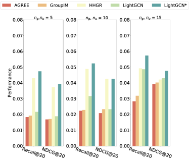
(a) Weeplaces

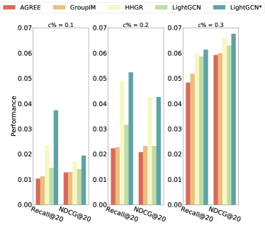
(b) Weeplaces

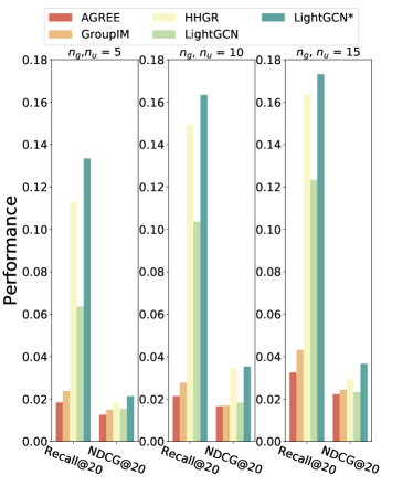
(c) CAMRa2011

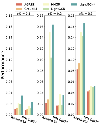
(d) CAMRa2011

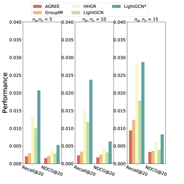
(e) Douban

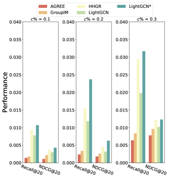
(f) Douban

Figure 3: Recommendation performance under different interacted numbers $n_{u}$ and $n_{g}$ (Cf. Fig 3(a), Fig 3(c) and Fig 3(e)), and under different sparse rate $c$% (Cf. Fig 3(b), Fig 3(d) and Fig 3(f)).

4.3 Ablation Study (Q2)

We perform the ablation study to explore whether each component in ${\rm SGG}$ is reasonable for the good recommendation performance. To this end, we report the recommendation performance for ${\rm SGG}$ and its variant model in Table 4. We find that: (1) Basic-GNN and Meta-GNN is consistently superior than the vanilla GNNs, which indicates the effectiveness of the proposed SSL tasks. (2) Among all the variant models, Meta-GNN performs the best, which indicates enhancing the cold-start neighbors’ embedding quality is much more important. (3) GNN* performs the best, which verifies the superiority of combining these SSL tasks.

Table 4: Ablation study for SGG with sparse rate $c$%= 0.1, layer size $L$=3 and neighbor size $K$=5.

Methods	Weeplaces		CAMRa2011		Douban
	Recall	NDCG	Recall	NDCG	Recall	NDCG
${\rm GCMC}$	0.0312	0.0083	0.0348	0.0171	0.0036	0.0025
${\rm Basic}$-${\rm GCMC}$	0.0412	0.0293	0.0561	0.0278	0.0045	0.0028
${\rm Meta}$-${\rm GCMC}$	0.0441	0.0328	0.0826	0.0319	0.0048	0.0031
${\rm GCMC*}$	0.0513	0.0448	0.1112	0.0394	0.0053	0.0038
${\rm NGCF}$	0.0336	0.0093	0.0288	0.0177	0.0043	0.0028
${\rm Basic}$-${\rm NGCF}$	0.0390	0.0241	0.0971	0.0233	0.0068	0.0041
${\rm Meta}$-${\rm NGCF}$	0.0480	0.0382	0.1172	0.0319	0.0121	0.0042
${\rm NGCF*}$	0.0486	0.0413	0.1256	0.0342	0.0133	0.0043
${\rm LightGCN}$	0.0316	0.0233	0.1036	0.0183	0.0118	0.0032
${\rm Basic}$-${\rm LightGCN}$	0.0373	0.0318	0.1252	0.0210	0.0181	0.0038
${\rm Meta}$-${\rm LightGCN}$	0.0475	0.0415	0.1556	0.0312	0.0232	0.0049
${\rm LightGCN*}$	0.0523	0.0426	0.1634	0.0353	0.0237	0.0063

4.4 Study of SGG (Q3)

4.4.1 Effectiveness of Meta-Learning Setting.

As mentioned in Section 3.1, we train ${\rm SGG}$ under the meta-learning setting. In order to examine whether the meta-learning setting can benefit the recommendation performance and have satisfactory time complexity, we compare ${\rm SGG}$ and the vanilla GNN model with a variant model ${\rm SGG}$-M, which removes the meta-learning setting. More Concretely, in ${\rm SGG}$-M, for each group/user/item, we do not sample $K$ neighbors, but instead directly using their first-order and high-order neighbors to perform graph convolution. We report the average recommendation performance, the average training time in each epoch and the average convergent epoch in Table 5. Based on the results, we find that ${\rm SGG}$ is consistently superior than ${\rm SGG}$-M, and has much more smaller training time in each epoch, much faster converges speed. This indicates training ${\rm SGG}$ in the meta-learning setting can not only improve the model performance, but also improve the training efficiency.

Table 5: Recommendation performance, training time per epoch and convergent epochs w/wo meta-learning setting.

Dataset	Weeplace				CAMRa2011
Method	Recall	NDCG	Time	Epoch	Recall	NDCG	Time	Epoch
GCMC	0.0312	0.0083	188.6s	31	0.0348	0.0171	51.8s	30
GCMC*-M	0.0509	0.0453	721.3s	30	0.1021	0.0382	172.6s	22
GCMC*	0.0513	0.0448	499.6s	12	0.1112	0.0394	112.3s	10
NGCF	0.0336	0.0093	182.6s	30	0.0288	0.0177	58.7s	26
NGCF*-M	0.0465	0.0403	700.2s	20	0.1123	0.0325	166.3s	13
NGCF*	0.0486	0.0413	489.7s	8	0.1256	0.0342	100.8s	8
LightGCN	0.316	0.0233	179.2s	30	0.1036	0.0183	48.3s	30
LightGCN*-M	0.0511	0.0402	683.6s	18	0.1435	0.0329	153.8s	18
LightGCN*	0.0523	0.0426	483.4s	10	0.1634	0.0353	99.3s	6

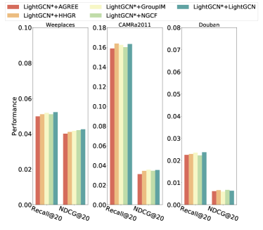
(a) Recommendation performance

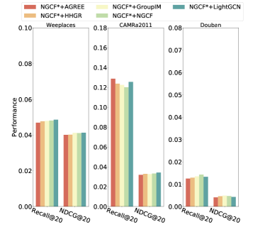
(b) Recommendation performance

Figure 4: Sensitive analysis of ground-truth embeddings.

4.4.2 Effectiveness of Ground-truth Embedding.

Notably, in Section 3.1, we select any group recommendation models to learn the ground-truth embeddings. Here we explore whether the ground-truth embeddings obtained by different models can affect the performance of ${\rm SGG}$. To this end, we use competitive baselines to learn the ground-truth embeddings as proposed in Section 4.1.3, and report the performance of NGCF* and LightGCN* in Figure 4. Notation NGCF*-AGREE denotes ${\rm SGG}$ is equipped with the ground-truth embeddings, which are obtained by AGREE. Other notations are defined in a similar way. The results show that the performance of ${\rm SGG}$ is almost the same under different ground-truth embeddings, the reason is that traditional recommendation methods are able to learn accurate embeddings for the nodes with enough interactions.

Table 6: Recommendation performance, training time for each epoch and convergent epochs under the multi-task learning or pre-training paradigms.

Dataset	Weeplaces				CAMRa2011
Method	Recall	NDCG	Time	Epoch	Recall	NDCG	Time	Epoch
GCMC*-P	0.0428	0.0409	201.0s	28	0.1008	0.0317	56.29s	26
GCMC*	0.0513	0.0448	499.6s	12	0.1112	0.0394	112.3s	10
NGCF*-P	0.0411	0.0388	203.1s	28	0.1182	0.0318	60.2s	28
NGCF*	0.0486	0.0413	489.7s	8	0.1256	0.0342	100.8s	8
LightGCN*-P	0.0487	0.0386	189.3s	28	0.1525	0.0327	50.1s	28
LightGCN*	0.0523	0.0426	483.4s	10	0.1634	0.0353	99.3s	6

4.4.3 Multi-task Learning Vs Pre-training.

We report the recommendation performance under the two training paradigms as proposed in Section 3.3. For the pre-training paradigm, we first pre-train the SSL task on $D_{T}$ and then fine-tune ${\rm SGG}$ on $D_{N}$ with the recommendation task. We use notation ${\rm SGG}$-P to denote this training paradigm. For the multi-task learning paradigm, we directly train the SSL task and the recommendation task on $D_{T}$ and $D_{N}$. We report the recommendation performance, the average training time in each epoch and the average convergent epoch in Table 6. Based on the results, we find that: (1) ${\rm SGG}$-P performs worse than ${\rm SGG}$, but still better than other baselines (cf. Table 3). This shows the SSL task can benefit the recommendation performance. However, jointly training the SSL task and the recommendation task is better than the pre-training & fine-tuning paradigm, since the two tasks can enhance with each other, this finding is the same with previous findings [45]. (2) Compared with ${\rm SGG}$-P, ${\rm SGG}$ has faster convergence speed. Although ${\rm SGG}$-P has smaller training time per epoch, it still has larger total training time than ${\rm SGG}$. This verifies the multi-task learning paradigm can speed up the model convergence.

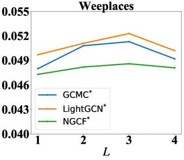
(a) Recall@20

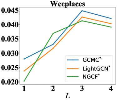
(b) NDCG@20

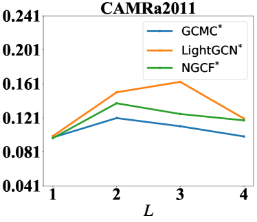
(c) Recall@20

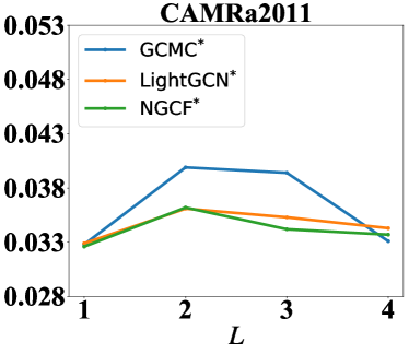
(d) NDCG@20

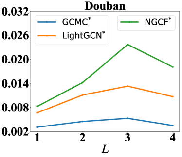
(e) Recall@20

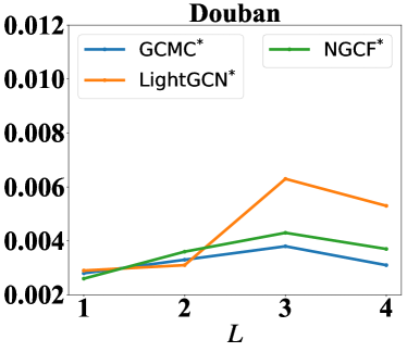
(f) NDCG@20

Figure 5: Recommendation performance under different layer $L$ $c$%=0.1 and $K$=5.

4.4.4 Hyper-parameter analysis.

Here we explore whether ${\rm SGG}$ is sensitive to the layer depth $L$, the neighbor size $K$, and the hyperparameter $\lambda 1$. We select LightGCN*, NGCF* and GCMC*, report their performances under different layer depth $L$ in Figure 5, under different neighbor size $K$ in Figure 6, and under different hyperparameter $\lambda_{1}$ in Figure 7. The results show that:

• In terms of $L$, the performance increases from 1 to 3 and drops from 3 to 4. When $L$ equals to 3, ${\rm SGG}$ always has the best performance. This indicates using proper layer size can benefit the recommendation task.

• In terms of $K$, the performance increases from 3 to 8 and drops from 8 to 12. When $K$ is 8, ${\rm SGG}$ can always achieve the best performance. This indicates incorporating proper size of neighbors can benefit the recommendation task.

• In terms of the balancing parameter $\lambda_{1}$, we report the recommendation performance of LightGCN*, NGCF* and GCMC* on CAMRa2011 and Douban in Figure 7. The results show the performance increases from 0.01 to 1, and drops from 1 to 1.2. This indicates the auxiliary SSL tasks are as important as the main recommendation task.

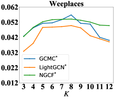
(a) Recall@20

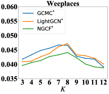
(b) NDCG@20

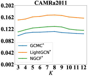
(c) Recall@20

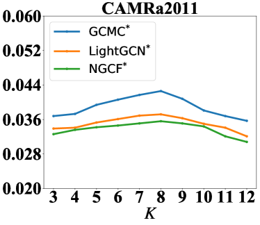
(d) NDCG@20

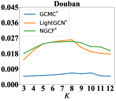
(e) Recall@20

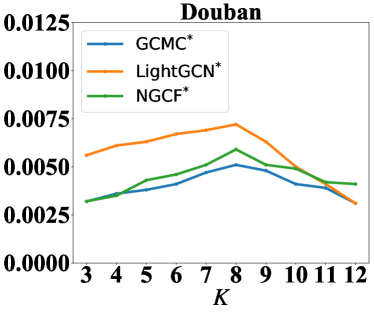
(f) NDCG@20

Figure 6: Recommendation performance under different neighbor size $K$. $c$%=0.1, $L$=3.

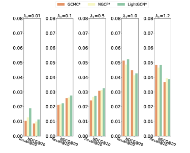
(a) Weeplaces

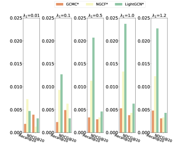
(b) Douban

Figure 7: Recommendation performance under different balancing parameter $\lambda_{1}$. $K$=5, $c$%=0.1 and $L$=3.

5 Related Work

5.1 Group Recommendation

The goal of group recommendation is to recommend proper items to a group. Different from Shared-account recommendation [58, 59], where the members in the shared-account is closely related, the members in the group may formed at hoc. Existing methods for group recommendation can be classified into the following two categories:

Score Aggregation Group Recommendation Strategy. This strategy pre-defines a scoring function to obtain the preference score of all members in a group on the target item. The scoring functions include average [2], least misery [5] and maximum satisfaction [3]. However, due to the static recommendation process of the predefined functions, these methods easily fall into local optimal solutions.

Profile Aggregation Group Recommendation Strategy. This strategy aggregates the group members’ profiles and feeds the fused group profile into individual recommendation models. Essentially, probabilistic generative models and deep learning based models are proposed to aggregate the group profile. The generative model first selects group members for a target group, and then generates items based on the selected members and their associated hidden topics [4, 7, 8]. The deep learning based model conducts attention mechanism to assign each user an attention weight, which denotes the influence of group member in deciding the group’s choice on the target item [10, 11, 1]. However, both of these two methods suffer from the data sparsity issue. Recently, researches propose GNN-based recommendation models, which incorporate high-order collaborative signals in the built graph [12, 13, 14, 54] or hypergraph [15, 16, 57]. Moreover, Zhang et al. [46] propose hypergraph convolution network (HHGR) with self-supervised node dropout strategy. However, the GNNs still can not strengthen the cold-start neighbors’ embedding quality. Motivated by recent works which leverage the SSL technique to solve the cold-start problems [54, 55, 56, 57] such as PT-GNN [17] and SGL [53], we propose the group/user/item embedding reconstruction task under the meta-learning setting, and further incorporate an embedding enhancer to improve the embedding quality. Notably, our work is related to PT-GNN [17], which reconstructs the cold-start user/item embeddings for personalized recommendation. Different from PT-GNN, the group embedding reconstruction in ${\rm SGG}$ is much more complex, as the decision process of a group is much more complicated than an individual user. Besides, the group representation not only depends on the group members’ preferences, but also relies on the group-level preferences towards items and collaborative group signals. Thus, the group embedding reconstruction process is much more complicated than user/item embedding reconstruction. Recently, Chen et al [57] propose CubeRec, which uses the hypercube to model the group member decision process to enhance the group embedding. Although both CubeRec and ${\rm SGG}$ is to enhance the group representation, CubeRec takes subspace to strengthen the group embedding, while ${\rm SGG}$ views the group embedding as a single point and directly leverage SSL technique to enhance the group embedding.

6 Conclusion

We present a self-supervised graph learning framework for group recommendation. In this framework, we design the user/item/group embedding reconstruction task with GNNs under the meta-learning setting, We further introduce an embedding enhancer to strengthen the GNNs’ aggregation ability, which can improve the high-order cold-start neighbors’ embedding quality. Comprehensive experiments show the superiority of our proposed framework than the state-of-the-art methods. The limitation of this work is that the proposed model is not a general pre-training model that can be applied to new recommendation datasets. In the future, our goal is to design a general pre-training recommendation model that can be applied to different datasets, we hope to achieve the same effect as the natural language pre-training model BERT [60]. More concretely, we will dedicate to learn the structure and semantic information in the user-item-group heterogeneous graph, and transfer the learned information into new datasets.

References

- [1] Yin, H., Wang, Q., Zheng, K., Li, Z., Yang, J., Zhou, X. ICDE’19 (pp. 566-577). Social influence-based group representation learning for group recommendation. (2019).
- [2] Baltrunas, L., Makcinskas, T., Ricci, F. Recsys’10 (pp. 119-126) Group recommendations with rank aggregation and collaborative filtering. (2010).
- [3] Boratto, L., Carta, S. State-of-the-art in group recommendation and new approaches for automatic identification of groups. Information retrieval and mining in distributed environments (pp. 1-20). (2010).
- [4] Liu, X., Tian, Y., Ye, M., Lee, W. C. CIKM’12 (pp. 674-683) Exploring personal impact for group recommendation. (2012).
- [5] Amer-Yahia, S., Roy, S. B., Chawlat, A., Das, G., Yu, C. VLDB’09 (pp. 754-765) Group recommendation: Semantics and efficiency. (2009).
- [6] Vinh Tran, L., Nguyen Pham, T. A., Tay, Y., Liu, Y., Cong, G., Li, X. SIGIR’19 (pp. 255-264) Interact and decide: Medley of sub-attention networks for effective group recommendation. (2019).
- [7] Ye, M., Liu, X., Lee, W. C. SIGIR’12 (pp. 671-680) Exploring social influence for recommendation: a generative model approach. (2012).
- [8] Yuan, Q., Cong, G., Lin, C. Y. SIGKDD’14 (pp. 163-172). COM: a generative model for group recommendation. (2014).
- [9] Vaswani, A., Shazeer, N., Parmar, N., Uszkoreit, J., Jones, L., Gomez, A. N., … Polosukhin, I. NIPS’17. Attention is all you need. (2017)
- [10] Cao, D., He, X., Miao, L., An, Y., Yang, C., Hong, R. SIGIR’18 (pp. 645-654). Attentive group recommendation. (2018).
- [11] Cao, D., He, X., Miao, L., Xiao, G., Chen, H., Xu, J. IEEE Trans Knowl Data Eng, 33(3), 1195-1209. Social-enhanced attentive group recommendation. (2019).
- [12] Guo, L., Yin, H., Wang, Q., Cui, B., Huang, Z., Cui, L. ICDE’20 (pp. 121-132). Group recommendation with latent voting mechanism. (2020).
- [13] Wang, W., Zhang, W., Rao, J., Qiu, Z., Zhang, B., Lin, L., Zha, H. SIGIR’20 (pp. 1449-1458). Group-aware long-and short-term graph representation learning for sequential group recommendation. (2020).
- [14] He, Z., Chow, C. Y., Zhang, J. D. SIGIR’20 (pp. 649-658). GAME: Learning graphical and attentive multi-view embeddings for occasional group recommendation. (2020).
- [15] Yu, J., Yin, H., Li, J., Wang, Q., Hung, N. Q. V., Zhang, X. WWW’21 (pp. 413-424). Self-supervised multi-channel hypergraph convolutional network for social recommendation. (2021).
- [16] Guo, L., Yin, H., Chen, T., Zhang, X., Zheng, K. ACM Trans Inf Syst, 40(1), 1-27. Hierarchical hyperedge embedding-based representation learning for group recommendation. (2021)
- [17] Hao, B., Zhang, J., Yin, H., Li, C., Chen, H. WSDM’21 (pp. 265-273). Pre-training graph neural networks for cold-start users and items representation. (2021).
- [18] Liu, Y., Yang, S., Lei, C., Wang, G., Tang, H., Zhang, J., … Miao, C. MM’21 (pp. 2853-2861). Pre-training graph transformer with multimodal side information for recommendation. (2021).
- [19] Qiu, J., Chen, Q., Dong, Y., Zhang, J., Yang, H., Ding, M., … Tang, J. SIGKDD’20 (pp. 1150-1160). Gcc: Graph contrastive coding for graph neural network pre-training. (2020).
- [20] Hu, Z., Dong, Y., Wang, K., Chang, K. W., Sun, Y. SIGKDD’20 (pp. 1857-1867). Gpt-gnn: Generative pre-training of graph neural networks. (2020).
- [21] Sun, F. Y., Hoffmann, J., Verma, V., Tang, J. ICLR’20. Infograph: Unsupervised and semi-supervised graph-level representation learning via mutual information maximization. (2019).
- [22] He, X., He, Z., Song, J., Liu, Z., Jiang, Y. G., Chua, T. S. IEEE Trans Knowl Data Eng, 30(12), 2354-2366. Nais: Neural attentive item similarity model for recommendation. (2018).
- [23] Liu, C., Wang, X., Lu, T., Zhu, W., Sun, J., Hoi, S. AAAI’19 (pp. 208-215). Discrete social recommendation. (2019).
- [24] Sun, P., Wu, L., Wang, M. SIGIR’18 (pp. 185-194). Attentive recurrent social recommendation. (2018).
- [25] Gao, L., Wu, J., Qiao, Z., Zhou, C., Yang, H., Hu, Y. CIKM’16 (pp. 1941-1944). Collaborative social group influence for event recommendation. (2016).
- [26] Yin, H., Zou, L., Nguyen, Q. V. H., Huang, Z., Zhou, X. ICDE’18 (pp. 929-940). Joint event-partner recommendation in event-based social networks. (2018).
- [27] Sankar, A., Wu, Y., Wu, Y., Zhang, W., Yang, H., Sundaram, H. SIGIR’20 (pp. 1279-1288). Groupim: A mutual information maximization framework for neural group recommendation. (2020).
- [28] He, X., Deng, K., Wang, X., Li, Y., Zhang, Y., Wang, M. SIGIR’20 (pp. 639-648). Lightgcn: Simplifying and powering graph convolution network for recommendation. (2020).
- [29] Hamilton, W., Ying, Z., Leskovec, J. NIPS’17. Inductive representation learning on large graphs. (2017).
- [30] Hao, B., Zhang, J., Li, C., Chen, H., Yin, H. ECML-PKDD’20 (pp. 36-51) Recommending Courses in MOOCs for Jobs: An Auto Weak Supervision Approach. (2020).
- [31] Rendle, S., Freudenthaler, C., Gantner, Z., Schmidt-Thieme, L. UAI’09. BPR: Bayesian personalized ranking from implicit feedback. (2009).
- [32] De Pessemier, T., Dooms, S., Martens, L. Comparison of group recommendation algorithms. MULTIMED TOOLS APPL (2016).
- [33] Vinyals, O., Blundell, C., Lillicrap, T., Wierstra, D. NIPS’16. Matching networks for one shot learning. (2016).
- [34] Chen, J., Ma, T., Xiao, C. ICLR’18. Fastgcn: fast learning with graph convolutional networks via importance sampling. (2018).
- [35] Hu, Z., Chen, T., Chang, K. W., Sun, Y. ACL’19. Few-shot representation learning for out-of-vocabulary words. (2019).
- [36] Zaheer, M., Kottur, S., Ravanbakhsh, S., Poczos, B., Salakhutdinov, R. R., Smola, A. J. NIPS’17. Deep sets. (2017).
- [37] Zhang, J., Hao, B., Chen, B., Li, C., Chen, H., Sun, J. AAAI’19 (pp. 435-442). Hierarchical reinforcement learning for course recommendation in MOOCs. (2019).
- [38] Cremonesi, P., Koren, Y., Turrin, R. Recsys’10 (pp. 39-46).Performance of recommender algorithms on top-n recommendation tasks. (2010).
- [39] Rakesh, V., Lee, W. C., Reddy, C. K. WSDM’16 (pp. 257-266). Probabilistic group recommendation model for crowdfunding domains. (2016).
- [40] Wu, Y., Liu, H., Yang, Y. KDIR (pp. 49-58). Graph Convolutional Matrix Completion for Bipartite Edge Prediction. (2018).
- [41] Kipf, T. N., Welling, M. ICLR’17. Semi-supervised classification with graph convolutional networks. (2017).
- [42] Wang, X., He, X., Wang, M., Feng, F., Chua, T. S. SIGIR’19. (pp. 165-174). Neural graph collaborative filtering. (2019).
- [43] Gilmer, J., Schoenholz, S. S., Riley, P. F., Vinyals, O., Dahl, G. E. ICML’17 (pp. 1263-1272). Neural message passing for quantum chemistry. (2017).
- [44] Glorot, X., Bengio, Y. (2010, March). IJCAI’10 (pp. 249-256). Understanding the difficulty of training deep feedforward neural networks. (2010).
- [45] Wu, J., Wang, X., Feng, F., He, X., Chen, L., Lian, J., Xie, X. SIGIR’21 (pp. 726-735). Self-supervised graph learning for recommendation. (2021).
- [46] Zhang, J., Gao, M., Yu, J., Guo, L., Li, J., Yin, H. CIKM’21 (pp. 2557-2567). Double-Scale Self-Supervised Hypergraph Learning for Group Recommendation. (2021).
- [47] Chen, T., Kornblith, S., Norouzi, M., Hinton, G. ICML’20 (pp. 1597-1607). A simple framework for contrastive learning of visual representations. (2020).
- [48] Yang, Q., Hu, S., Zhang, W., Zhang, J. Int. J. Intell. Attention mechanism and adaptive convolution actuated fusion network for next POI recommendation. (2022).
- [49] Zhang, X., Ma1, H., Gao, Z., Li, Z., Chang, L. Int. J. Intell. Exploiting cross-session information for knowledge-aware session-based recommendation via graph attention networks. (2022).
- [50] Yu, X., Che, X., Mao, Q., Gong, Z., Fu, W., Zheng, X. Int. J. Intell. PF-ITS: Intelligent traffic service recommendation based on DeepAFM model. 30(1), 1-14. (2022).
- [51] Hung, N. Q. V., Viet, H. H., Tam, N. T., Weidlich, M., Yin, H., & Zhou, X. IEEE Trans Knowl Data Eng, 30(1), 1-14. Computing crowd consensus with partial agreement. (2017).
- [52] Nguyen, T. T., Duong, C. T., Weidlich, M., Yin, H., & Nguyen, Q. V. H. IJCAI’17. Retaining data from streams of social platforms with minimal regret. (2017).
- [53] Wu, J., Wang, X., Feng, F., He, X., Chen, L., Lian, J., & Xie, X. SIGIR’21 (pp. 726-735). Self-supervised graph learning for recommendation. (2021).
- [54] Yin, H., Wang, Q., Zheng, K., Li, Z., & Zhou, X. IEEE Trans Knowl Data Eng. Overcoming data sparsity in group recommendation. (2020).
- [55] Hao, B., Yin, H., Zhang, J., Li, C., & Chen, H. (2021). ACM Trans Inf Syst. A Multi-Strategy based Pre-Training Method for Cold-Start Recommendation. (2022).
- [56] Hao, B., Zhang, J., Li, C., & Chen, H. APWeb-WAIM’20 (pp. 363-377). Few-Shot Representation learning for Cold-Start users and items. (2020).
- [57] Chen, T., Yin, H., Long, J., Nguyen, Q. V. H., Wang, Y., & Wang, M. SIGIR’22. Thinking inside The Box: Learning Hypercube Representations for Group Recommendation. (2022).
- [58] Guo, L., Zhang, J., Chen, T., Wang, X., & Yin, H. IEEE Trans Knowl Data Eng. Reinforcement Learning-enhanced Shared-account Cross-domain Sequential Recommendation. (2022).
- [59] Guo, L., Tang, L., Chen, T., Zhu, L., Nguyen, Q. V. H., & Yin, H. IJCAI’21. DA-GCN: a domain-aware attentive graph convolution network for shared-account cross-domain sequential recommendation. (2021).
- [60] Devlin, J., Chang, M. W., Lee, K., & Toutanova, K. NAACL-HIT’19. (pp. 4171-4186). Bert: Pre-training of deep bidirectional transformers for language understanding. (2019).