Harsha et al.

Deep Policy Iteration for Inventory Management

Deep Policy Iteration with Integer Programming for Inventory Management

Pavithra Harsha, Ashish Jagmohan, Jayant Kalangnanam, Brian Quanz IBM Research, Thomas J. Watson Research Center, Yorktown Heights, NY 10598, USA Divya Singhvi NYU Leonard N. Stern School of Business, NY 10012, USA

Problem Definition: In this paper, we present a Reinforcement Learning (RL) based framework for optimizing long-term discounted reward problems with large combinatorial action space and state dependent constraints. These characteristics are common to many operations management problems, e.g., network inventory replenishment, where managers have to deal with uncertain demand, lost sales, and capacity constraints that results in more complex feasible action spaces. Our proposed Programmable Actor Reinforcement Learning (PARL) uses a deep-policy iteration method that leverages neural networks (NNs) to approximate the value function and combines it with mathematical programming (MP) and sample average approximation (SAA) to solve the per-step-action optimally while accounting for combinatorial action spaces and state-dependent constraint sets. Results: We then show how the proposed methodology can be applied to complex inventory replenishment problems where analytical solutions are intractable. We also benchmark the proposed algorithm against state-of-the-art RL algorithms and commonly used replenishment heuristics and find that the proposed algorithm considerably outperforms existing methods by as much as 14.7% on average in various supply chain settings. Managerial Insights: We find that this improvement in performance of PARL over benchmark algorithms can be directly attributed to better inventory cost management, especially in inventory constrained settings. Furthermore, in a simpler back order setting where optimal replenishment policy is tractable, we find that the RL based policy also converges to the optimal policy. Finally, to make RL algorithms more accessible for inventory management researchers, we also discuss the development of a modular Python library that can be used to test the performance of RL algorithms with various supply chain structures. This library can spur future research in developing practical and near-optimal algorithms for inventory management problems.

Multi Echelon Inventory Management, Inventory Replenishment, Deep Reinforcement Learning This paper is under preparation.

1 Introduction

Inventory and supply chain management have seen a tremendous shift over the past decade. With the advent of online e-commerce, supply chains have become more and more complex and global with increasingly connected physical flows (young_2022). Naturally, the cost of managing these supply chains have increased over the years. Furthermore, the pandemic has lead to an increased spending in managing such complex supply chains. In fact, a recent Wall Street Journal report states that US business logistics costs increased as much as 22% year-on-year (young_2022). One potential promising direction for managing such complex supply chains is to use Artificial Intelligence (AI) based inventory management solutions and explore the benefits it can provide.

AI and Reinforcement learning (RL) has led to considerable breakthroughs in diverse areas such as games (mnih2013playing), robotics (kober2013reinforcement) and others. RL provides a systematic framework to solve sequential decision making problems with very limited domain knowledge. In fact, one can leverage several state-of-the-art, open-source RL methods to learn a very good policy that maximizes long-run rewards of many sequential decision problems at hand. Therefore, it is not surprising that RL has recently also been applied to similar problems in various domains such as healthcare (yu2019reinforcement), supply chains (gijsbrechts2018can, oroojlooyjadid2021deep, sultana2020reinforcement) and more. Yet enterprise level operations applications of RL remains limited and quite challenging.

Consider typical operations management (OM) problems such as inventory management and network revenue management. These problems are generally characterized by large action spaces, often well-defined state-dependent action constraints and rewards, and underlying stochastic transition dynamics. For example, a firm managing the inventory across a network of nodes in the supply chain has to decide how much inventory to place across the different nodes of the network. To accomplish this efficiently, the firm has to overcome various challenges. This includes accounting for (i) the uncertain demand across the nodes in the network; (ii) a large set of locally feasible (and often combinatorial) actions since the firm decides on the number of units to allocate to different nodes; (iii) a large number of state-dependent constraints to ensure that the complete allocation vector is feasible; (iv) the trade-off between the immediate and the long term reward of actions.

RL methods use an environment, a live or simulated one, to sample the underlying uncertainty to generate reward trajectories, and in-turn estimates of different action policies by understanding the trade-off between long term and short term rewards. Nevertheless, large combinatorial action spaces with state-dependent constraints, as in the case of the OM problems described above, render enumeration based RL techniques over the action space, computationally intractable. Hence, in this paper, we present a specialized RL algorithm that resolves these challenges. In particular, we present a deep-policy iteration method that leverages neural networks (NNs) to approximate the value function and combines it with mathematical programming (MP) and sample average approximation (SAA) to solve the per-step-action optimally while accounting for combinatorial action spaces and state-dependent constraint sets. From an RL perspective, one can view this as replacing the actor in an actor-critic method with a math-programming based actor. We use this modified RL approach to provide benchmark solutions to inventory management problems with complexities that make analytical solutions even in simpler networks intractable (e.g. lost sales, fixed costs, dual sourcing, lead times in multi-echelon networks) and compare them with state-of-the art RL methods and popular supply chain heuristics.

1.1 Contributions

We make the following contributions through this work:

1. We present a policy iteration algorithm for dynamic programming problems with large action spaces and underlying stochastic dynamics that we call Programmable Actor Reinforcement Learning (PARL). In our framework, the value-to-go is represented as a sum of immediate reward and sum of future discounted rewards. The future discounted rewards are approximated with a NN that is fitted by generating value-to-go rewards from Monte-Carlo simulations. Then, we represent the NN and the immediate reward as an integer program which is used to optimize the per-step action. As the approximation improves, so does the per-step-action, which ensures that the learned policy eventually converges to the unknown optimal policy. The approach overcomes the enumeration challenges and allows an easy implementation of known contextual state dependent constraints.

2. We apply the proposed methodology to the problem of optimal replenishment decisions of a retailer with a network of warehouses and retail stores. Focusing on settings where analytical tractability is not guaranteed, we analyze and compare the performance of PARL under different supply chain network structures (multi-echelon distribution networks with and without dual-sourcing and with lost sales) and network sizes (single supplier and three retailers, to up to 20 heterogeneous retailers with multiple intermediary warehouses). We find that PARL is competitive, and in some cases outperforms, state of the art methods (14.6% improvement on average across different settings studied in this paper). Our numerical experiments provide a comprehensive benchmark results in these settings using different RL algorithms (SAC, TD3, PPO and A2C), as well as commonly used heuristics in various supply chain settings (specifically, base stock policies on an edge and on a serial path). We also perform additional numerical experiments to analyze the structure of the learned RL based replenishment policies and find that (i) in a simpler back-order setting, the RL policy is near optimal as it also learns an order up-to-policy and (ii) in the other more complex settings, the higher profitability is on account of improved cost management across the supply chain network.

3. Finally, we open source our supply chain environment as a Python library to allow researchers to easily implement and benchmark PARL and other state-of-the-art RL methods in various supply chain settings. Our proposed library is modular and allows for researchers to design supply chains networks with varying complexity (multi-echelon, dual sourcing), size (number of retailers and warehouses) and reward structure (back order and lost sales settings). While our objective is similar to hubbs2020or, we focus on inventory management problems specifically and provide more flexibility in the network design. We believe this library will make RL algorithms more accessible to the OR and inventory management community and spur future research in developing practical and near-optimal algorithms for inventory management problems.

1.2 Selected Literature Review

Our work is related to the following different streams of literature: (1) parametric policies, (2) approximate dynamic programming (ADP), (3) reinforcement learning (RL) and (4) mathematical programming based RL. As the literature in these topics, in general and even within the context of supply chain and inventory management specifically, is quite vast, we describe the state-of-the art with select related literature that is most related to the current work.

Parametric policies for inventory management:

The topic of inventory management has been studied for many years and it has a long history. The seminal work of scarf1960optimality shows that for a single node sourcing from a single supplier with infinite inventory, a constant lead time and an ordering cost with fixed and variable components, the optimal policy for back-ordered demand has a $(s,S)$ structure where $S$ is referred to as the order-up-level based on the inventory position (sum of on-hand inventory plus that in the pipeline, i.e., a collapsed inventory state) and $s$ an inventory position threshold, below which orders are placed. This $(s,S)$ policy is commonly referred to as the base stock policy.

For lost-sales demand settings, i.e., wherein demand excess of inventory is lost, when the lead times are non-zero, the structure of the optimal policy is unknown (zipkin2008old, zipkin2008structure) even in the single node setting sourcing from a single retailer. Moreover, base stock policies generally perform poorly (zipkin2008old), except when penalty costs are large, when inventory levels are high and stock-outs are rare. In general, the optimal policy depends on the full-inventory pipeline, unlike the state-space collapse that is possible in back order settings, and the complexity grows exponentially in lead time. In these settings, huh2009asymptotic, goldberg2016asymptotic respectively prove the following asymptotic optimality results (1) regarding the basestock policy when the penalties are high and (2) regarding the constant ordering policies when the lead times are large. xin2021understanding combines these results to propose a capped base stock policy that is asymptotically optimal as the lead time increases and shows good empirical performance for smaller lead times.

sheopuri2010new prove that the lost sales problem is a special case of dual sourcing problem (a retail node has access to 2 external suppliers), and hence base stock policies are not optimal, in general. In the dual sourcing setting, various heuristic policies similar to the lost sales setting extend the base stock policy with a constant order and/or cap that splits the order between the two suppliers depending on the inventory position across each have been independently proposed. These include the Dual-Index (veeraraghavan2008now), Tailored Base-Surge (allon2010global) and Capped Dual Index policies (sun2019robust).

Multi-echelon networks are those wherein there are multiple nodes, stages or echelons that hold inventory. Base stock policies are optimal only in special cases with back ordered demands without fixed costs with additional restrictive assumptions such as the a serial chain with back order penalty at the demand node (clark1960optimal) or the inability to hold demand in the warehouse in a 2-echelon distribution network (federgruen1984approximations). We refer the reader to de2018typology for an extensive review multi-echelon models studied based on variety of modeling assumptions and supply chain network structures.

Despite the non-optimality of base stock policies (the use of $(s,S)$ policies with a collapsed state space, i.e., via inventory positions), they are popular both in practice and in the literature. For example, ozer2008stock and rong2017heuristics propose competitive heuristics that compute the order-up to base stock levels for the multi-echelon distribution (tree) networks without fixed costs but with service level constraints and demand back ordering costs respectively, and show asymptotic optimality in certain dimensions in the 2-echelon case. agrawal2019learning propose a learning-based method to find the best base stock policy in a single node lost sales setting with regret guarantees. pirhooshyaran2020simultaneous develop a DNN-based learning approach to find the best order up-to levels in each link of a general supply chain network.

In this work, we present a deep RL approach and leverage it to solve a certain class of cost-based stochastic inventory management problems in settings where parametric optimal policies do not exist or are unknown, such as the multi-echelon supply chains with fixed costs, capacities, lost sales and dual sourcing. In these settings, we provide new empirical benchmarks wherein the algorithm we propose is able to outperform commonplace heuristics that are based on the base-stock policy.

Approximate Dynamic Programming (ADP) and Reinforcement Learning (RL):

Our work is also related to the broad field of ADP (bertsekas2012dynamic, powell2007approximate). This generally focuses on solving the Bellman’s equation (1) and has been an area of active research for many years. ADP methods typically use an approximation of the value function to optimize over computationally intractable dynamic programming problems. Popular algorithms can be classified into two types: model-aware and model-agnostic. Model-aware approaches use information on underlying system dynamics (known transition function and immediate reward) to estimate value-to-go and popular approaches include value iteration and policy iteration. These algorithms essentially start with arbitrary estimates of the value-to-go and iteratively improve these estimates to eventually converge to the unknown optimal policy. We refer the interested readers to gijsbrechts2018can for an excellent review of ADP based approaches for inventory management.

Model-agnostic approaches circumvent the issue of partial or no knowledge of the underlying system dynamics by trial-and-error using an environment that generates immediate-reward and state-transitions, given the current state and a selected action. This latter framework is popularly referred to as Reinforcement Learning (RL) (sutton2018reinforcement). Note that RL methods themselves are also categorized into model-based RL and model-free RL wherein in process of learning the optimal policy via the environment, the transition functions are also learned in the former method and not learned in the latter method.

In this paper, we focus on model-free RL methods. One of the popular model-free RL algorithms is Q-learning, wherein the value of each state-action pair is estimated using the collected trajectory of state and rewards based on different actions and then the optimal action is obtained by an exhaustive search. In classical RL methods, a set of features are chosen and polynomial functions of those features are used to approximate the value function (van1997neuro). This had limited success initially, but after the deep-learning revolution and the availability of significant compute, the deep-RL (DRL) methods regained significant popularity and success as neural-nets were used to approximate the value function, thereby automating the step of feature and function selection.This led to many algorithmic breakthroughs including the development of a family of policy gradient methods called the actor-critic method (mnih2016asynchronous), in which neural networks are used to approximate both the value function and the policy itself - the policy with an actor network which encodes a distribution over actions. Despite their successes, DRL and actor-critic approaches suffer from several challenges, such as lack of robust convergence properties, high sensitivity to hyper parameters, high sample complexity, and function approximation errors in their networks leading to sub-optimal policies and incorrect value estimation (see, for discussions, pmlr-v80-haarnoja18b, maei2009convergent, fujimoto2018addressing, duan2016benchmarking, schulman2017proximal, henderson2018deep, lillicrap2016continuous). To address these different issues, new variations of the actor-critic approach continue to be proposed, such as Proximal Policy Optimization (PPO), which tries to avoid convergence to a sub-optimal solution while still enabling substantial policy improvement per update by constraining the divergence of the updated policy from the old one (schulman2017proximal), and Soft Actor-Critic (SAC), which tries to improve exploration via entropy regularization to improve hyper parameter robustness and prevent convergence to bad local optima while accelerating policy learning overall (pmlr-v80-haarnoja18b).

The current work is complimentary to this literature since we provide a principled way of factoring in known constraints and immediate reward explicitly in training, as opposed to having to implicitly infer/learn them. Additionally, our framework, as mentioned earlier, can be viewed as replacing the actor in the actor-critic method with a mixed-integer program. These aspects of our proposed approach potentially help address the known issues with actor critic methods, such as reducing the sample complexity, improving robustness and reducing the risk of convergence to poor solutions, and removing the dependence on function approximation of the policy network which may be inaccurate due to over or under fitting or sampling from the data (e.g., due to under-exploration or sub-optimal convergence).

RL for inventory management:

Early work that shows the benefits of RL for multi-echelon inventory management problems include van1997neuro, giannoccaro2002inventory, stockheim2003reinforcement. There has been a recent surge in using DNN-based reinforcement learning techniques to solve supply chain problems (gijsbrechts2018can, oroojlooyjadid2021deep, sultana2020reinforcement, hubbs2020or). A DNN-based actor-critic method to solve the inventory management problem was studied in gijsbrechts2018can for the case of single node lost sales and dual sourcing settings, as well as multi-echelon settings, and showed improved performance in the latter setting. oroojlooyjadid2021deep show how RL can be used to solve the classical bear game problem where agents in a serial supply chain compete for limited supply. More recently sultana2020reinforcement use a multi-agent actor-critic framework to solve an inventory management problem for a large number of products in a multi-echelon setting. Similarly, qi2020practical develop a practical end-to-end method for inventory management with deep learning.  hubbs2020or show the benefit of RL methods over static policies like base stock in a serial supply chain for a finite horizon problem. We also refer the interested readers to an excellent overview and roadmap for using RL for inventory management in boute2021deep. Unlike these papers, we adopt a mathematical programming-based RL actor and show the benefit over vanilla DRL approaches in the inventory management setting.

Mathematical programming (MP) based RL actor:

MP techniques have recently been used for optimizing actions in RL settings with DNN-based function approximators and large action spaces. They leverage MP to optimize a mixed-integer (linear) problem (MIP) over a polyhedral action space using commercially available solvers such as CPLEX and Gurobi. A number of papers show how trained ReLU-based DNNs can be expressed as an MP with tjandraatmadja2020convex, anderson2020strong also providing ideal reformulations that improve computational efficiencies with a solver. ryu2019caql propose a Q-learning framework to optimize over continuous action spaces using a combination of MP and a DNN actor. delarue2020reinforcement, van2019approximate, xu2020deep show how to use ReLU-based DNN value functions to optimize combinatorial problems (e.g., vehicle routing) where the immediate rewards are deterministic and the action space is vast. In this paper, we apply it to inventory management problems where the rewards are uncertain.

2 Model and Performance Metrics

Model and notation:

We consider an infinite horizon discrete-time discounted Markov decision process (MDP) with the following representation: states $s\in\mathcal{S}$, actions $a\in\mathcal{A}(s)$, uncertain random variable $D\in\mathbb{R}^{\texttt{dim}}$ with probability distribution $P(D=d|s)$ that depends on the context state $s$, reward function $R(s,a,D)$, distribution over initial states $\beta$, discount factor $\gamma$ and transition dynamics $s^{\prime}=\mathcal{T}(s,a,d)$ where $s^{\prime}$ represents the next state. A stationary policy $\pi\in\Pi$ is specified as a distribution $\pi(.|s)$ over actions $\mathcal{A}(s)$ taken at state $s$. Then, the expected return of a policy $\pi\in\Pi$ is given by $J^{\pi}=E_{s\sim\beta}V^{\pi}(s)$ where the value function is defined as

$$V^{\pi}(s)=\sum_{t=0}^{\infty}\mathbb{E}\left[\gamma^{t}R(s_{t},a_{t},D_{t})|s_{0}=s,\pi,P,\mathcal{T}\right]\,,$$

where the expectation is taken over both the immediate reward as well as the transition state. The optimal policy that maximizes the long term expected discounted reward is given by $\pi^{*}:=\arg\max_{\pi\in\Pi}J^{\pi}\,.$ Finally, by Bellman’s principle, the optimal policy is a unique solution to the following recursive equation:

$$V^{\pi^{*}}(s)=\max_{a\in\mathcal{A}(s)}\mathbb{E}_{D}\left[R(s,a,D)+V^{\pi^{*}}(\mathcal{T}(s,a,D))\right]\,.$$ (1)

As discussed in §1.2, solving (1) directly is computationally intractable due to the curse of dimensionality. We take a hybrid approach where a model determines the immediate reward but value-to-go is model-free and is determined using trial-and-error in a simulation environment. We discuss the algorithm in detail next.

2.1 Algorithm

We propose a monte-carlo simulation based policy-iteration framework where the learned policy is the outcome of a mathematical program which we refer to as PARL: Programming Actor Reinforcement Learning (see Algorithm 1 and an illustrative block diagram (Figure 1).

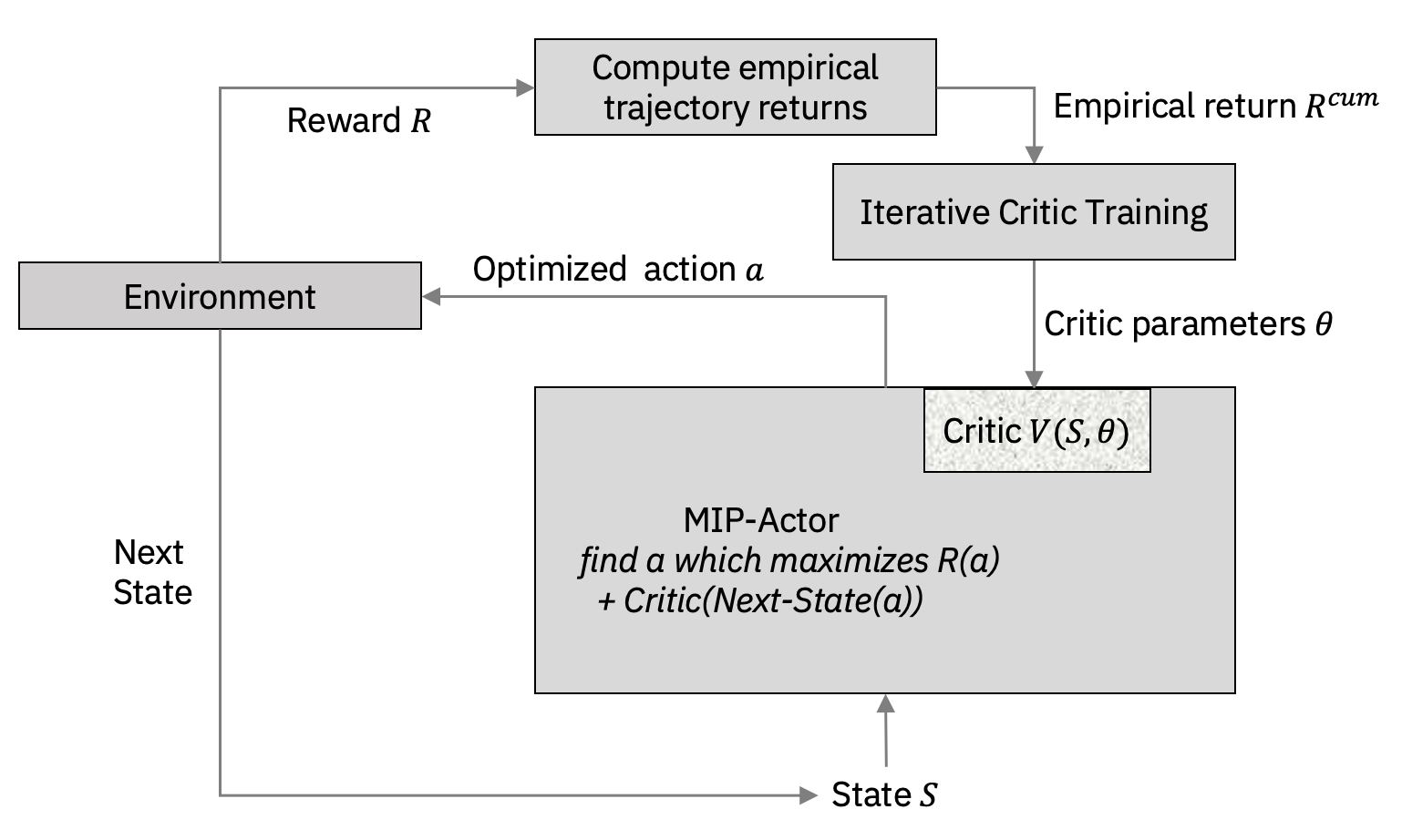
Figure 1: Block diagram illustration of the PARL algorithm

As is common in RL based methods, our framework assumes access to a simulation environment that generates state transitions and rewards, given an action and a current state. PARL is initialized with a random policy. The initial policy is iteratively improved over epochs with a learned critic (or the value function). In epoch j, policy $\pi_{j-1}$ is used to generate N sample paths, each of length T. At every time step, a tuple of {state ($s_{t}^{n}$), reward ($R_{t}^{n}$), next-state ($s_{t+1}^{n}$)} is also generated from the environment that is then used to estimate the value-to-go function $\hat{V}^{\pi_{j-1}}_{\theta}$. The value-to-go function is represented using a neural network parametrized by $\theta$ which is generated by solving the following error minimization problem:

$$\min_{\theta}\sum_{n=1}^{N}\sum_{t=1}^{T}\left(R^{cum,n}_{t}-\hat{V}^{\pi_{j}}_{\theta}(s_{t}^{n})\right)^{2}\,,$$

where the target variable $R^{cum,n}_{t}:=\sum_{i=t}^{T}\gamma^{i-t}R^{n}_{i}$ is the cumulative discounted reward from the state at time $t$ in sample path $n$, generated by simulating policy $\pi_{j-1}$. Once a $\hat{V}$ is estimated, the new policy using the trained value-to-go function is simply

$$\pi_{j}(s)=\arg\max_{a\in\mathcal{A}(s)}\mathbb{E}_{D}\left[R(s,a,D)+\gamma\hat{V}^{\pi_{j-1}}_{\theta}(\mathcal{T}(s,a,D))\right].$$ (2)

Problem (2) resembles Problem (1) except that the true value-to-go is replaced with an approximate value-to-go. Since, each iteration leads to an updated subsequent improved policy, we call it a policy iteration approach. Next, we discuss how to solve Problem (2) to get an updated policy in each iteration.

Problem (2) is hard to solve because of two main reasons. First, notice that $\hat{V}^{\pi_{j-1}}$ is a neural network which makes enumeration based techniques intractable, especially for settings where the actions space is large and combinatorial. And second, the objective function involves evaluating expectation over the distribution of uncertainty D that is analytically intractable to compute. We next discuss how PARL addresses each of these complexities.

2.2 Optimizing over a neural network

We first focus on the problem of maximization of the objective in (2). To simplify the problem we start by considering the case where demand D is deterministically known to be $d$. Then, Problem (2) can be written as

$$\max_{a\in\mathcal{A}(s)}R(s,a,d)+\gamma\hat{V}^{\pi_{j-1}}_{\theta}(\mathcal{T}(s,a,d))\,,$$

where we have removed the expectation over the uncertain demand $D$. Notice that the decision variable, a is an input to the value-to-go estimate represented by $\hat{V}$. Hence, optimizing over a involves optimizing over a neural network which is non-trivial. We take a math programming based approach to solve this problem. First, we assume that the value-to-go function is a trained $K$-layer feed forward ReLU-network with input state $s$ and satisfies the following equations $\forall k=2,\cdots,K,$

$$z_{1}=s,\ \hat{z}_{k}=W_{k-1}z_{k-1}+b_{k-1},\ z_{k}=\max\{0,\hat{z}_{k}\}\,$$

$$\hat{V}_{\theta}(s):=c^{T}\hat{z}_{K}\,.$$

Here, $\theta=(c,\{(W_{k},b_{k})\}_{k=1}^{K-1})$ are the parameters of the value-to-go estimator. Particularly, $(W_{k},b_{k})$ are the multiplicative and bias weights of layer $k$ and $c$ is the weight of the output layer (see Figure 2). Finally, $\hat{z}_{k},z_{k}$ denotes the pre- and post-activation values at layer $k$. ReLU activation at each neuron allows for a concise math programming representation that uses binary variables and big-M constraints (ryu2019caql, anderson2020strong). For completeness, we briefly describe the steps.

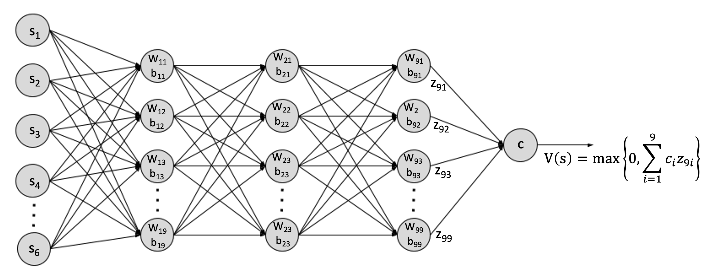
Figure 2: A representative NN that takes as an input, a 6-dimensional state space, and considers a 10 layer NN (including the output layer) with each internal layer containing 9 neurons. Each neuron is defined by weights (W) and bias (b), except for the output layer that is defined with parameter vector $c$. The output of each neuron uses ReLU activation and passes it as an input to the neurons in the subsequent layer.

Consider a neuron in the neural-network with parameters $(w,b)$. For example, in layer $k$ neuron $i$’s parameters are $(W_{k}^{i},b_{k}^{i})$. Assuming a bounded input $x\in[l,u]$, the output $z$ of that neuron can be obtained by solving following MP representation:

$$\texttt{P}(w,b,l,u):= \argmax_{x,z,y}~{}~{}0$$ (3)

$$z \geq w^{T}x+b$$

$$z \geq 0$$

$$z \leq w^{T}x+b-M^{-}(1-y)$$

$$z \leq M^{+}y$$

$$x \in[l,u]$$

$$y \in\{0,1\}\,.$$

Here,

$$M^{+}=\max_{x\in[l,u]}w^{T}x+b~{}~{}\&~{}~{}M^{-}=\min_{x\in[l,u]}w^{T}x+b\,,$$

are the maximum and minimum outputs of the neuron for any feasible input $s$. Note that $M^{+}$ and $M^{-}$ can be easily calculated by analyzing the component-wise signs on $w$. For example, let

$$\tilde{u}_{i}=\begin{cases}u_{i}~{}~{}\textit{if}~{}w_{i}\geq 0\\ l_{i},~{}~{}otherwise.\end{cases}$$

Similarly, let

$$\tilde{l}_{i}=\begin{cases}l_{i}~{}~{}\textit{if}~{}w_{i}\geq 0\\ u_{i},~{}~{}otherwise.\end{cases}$$

Then, simple algebra yields that $M^{+}=w^{T}\tilde{u}+b$ and $M^{-}=w^{T}\tilde{l}+b$. starting with the bounded input state $s$, the upper and lower bounds for subsequent layers can be obtained by assembling the $\max\{0,M^{+}\}$ and $\max\{0,M^{-}\}$ for each neuron from its prior layer. We will refer to them as $[l_{k},u_{k}]$ for every layer $k$. This MP reformulation of the neural network that estimates the value-to-go is crucial in our approach. Particularly, since we can also represent the immediate reward directly in terms of the decision $a$, and the feasible action set for any state is a polyhedron, we can now use the machinery of integer programming to solve Problem (2). We will make this connection more precise in §3 in the context of inventory management.

Next, we discuss how to tackle the problem of estimating expectation in Problem (2).

2.3 Maximizing expected reward with a large action space:

The objective in Problem (2) has an expectation that is taken over the uncertainty D. Note that the uncertainty in $D$ impacts both the immediate reward as well as the value-to-go via the transition function. Evaluating this expectation could be potentially hard since $D$ generally has a continuous distribution and we use a NN based value-to-go approximator. Hence, we take a SAA approach (kim2015guide) to solve it. Let $d_{1},d_{2},..d_{\eta}$ denote $\eta$ independent realizations of the uncertainty D. Then, SAA posits approximating the expectation as follows

$$\mathbb{E}_{D}[R(s,a,D)+\gamma\hat{V}^{\pi_{j-1}}_{\theta}(\mathcal{T}(s,a,D))]\approx\frac{1}{\eta}\sum_{i=1}^{\eta}R(s,a,d_{i})+\gamma\hat{V}^{\pi_{j-1}^{\eta}}_{\theta}(\mathcal{T}(s,a,d_{i}))\,.$$

Hence, Problem (2) becomes

$$\hat{\pi}^{\eta}_{j}(s)=\arg\max_{a\in\mathcal{A}(s)}\frac{1}{\eta}\sum_{i=1}^{\eta}R(s,a,d_{i})+\gamma\hat{V}^{\pi_{j-1}^{\eta}}_{\theta}(\mathcal{T}(s,a,d_{i}))\,.$$ (4)

Problem (4) involves evaluating the objective only at sampled points instead of all possible realizations. Assuming that for any $\eta$, the set of optimal actions is non empty, we show that as the number of samples, $\eta$ grows, the estimated optimal action converges to the optimal action. We make this statement precise in Proposition 2.1. The proof follows through standard results in the analysis of SAA and is provided in Appendix §LABEL:app:SAA_guarantee.

Proposition 2.1

Consider epoch $j$ of the PARL algorithm with a ReLU-network value function estimate $\hat{V}_{\theta}^{\pi_{j-1}}(s)$ for some fixed policy $\pi_{j-1}$. Suppose $\pi_{j},\hat{\pi}^{\eta}_{j}$ are the optimal policies as described in Problem (2) and its corresponding SAA approximation respectively. Then, $\forall~{}s$,

$$\lim_{\eta\to\infty}\hat{\pi}^{\eta}_{j}(s)=\pi_{j}(s).$$

Proposition 2.1 shows that the quality of the estimated policy improves as we increase the number of demand samples. Nevertheless, the computationally complexity of the problem also increases linearly with the number of samples: for each demand sample, we represent the DNN based value function estimation using binary variables and the corresponding set of constraints.

1:Initialize with random actor policy $\pi_{0}$.

2:for $j\in[\dot{\mathcal{T}}]$ do

3:     for (epoch) $n\in[N]$ do

4:         Play policy $\pi_{j-1}$ for $T(1-\epsilon)$ and random action for $\epsilon T$ steps starting with state $s_{0}^{n}\sim\beta$.

5:         Let $R^{cum,n}_{t}=\sum_{i=t}^{T}\gamma^{i-t}R_{i}^{n}$ and store tuple {$s_{t}^{n}$,$R_{t}^{cum,n}$} $\forall t=1,..,T$.

6:     end for

7:     Approximate a DNN value function approximator by solving

$$\hat{V}_{j}=\arg\min_{\theta}\sum_{n=1}^{N}\sum_{t=1}^{T}\left(R^{cum,n}_{t}-f(s_{t}^{n},\theta)\right)^{2}$$

8:     Sample $\eta$ realizations of the underlying uncertainty $D$ and obtain a new policy (as a lazy evaluation, as needed) by solving Problem (4)).

9:end for

Algorithm 1 PARL

Remark 2.2 (Incorporating Extra Information on the Underlying Uncertainty )

In many settings, the decision maker might have extra information on the underlying uncertainty $D$. In these cases, one can use specialized weighting schemes to estimate the expected value to go for different actions, given a state. For example, consider the case when the uncertainty distribution $P(D=d)$ is known and independent across different dimensions. Let $q_{1},q_{2},..q_{\eta}$ denote $\eta$ quantiles (for example, evenly split between 0 to 1). Also let $F_{j}~{}\&~{}f_{j},\forall j=1,2..,\texttt{dim}$, denote the cumulative distribution function and the probability density function of the uncertainty $D$ in each dimension respectively. Let $d_{ij}=F^{-1}_{j}(q_{i})~{}\&~{}\texttt{w}_{ij}=f_{j}(q_{i}),\forall i=1,2,..,\eta,j=1,2..,\texttt{dim}$ denote the uncertainty samples and their corresponding probability weights. Then, a single realization of the uncertainty is a dim dimensional vector $d_{i}=[d_{i1},..,d_{i,\texttt{dim}}]$ with associated probability weight $\texttt{w}^{pool}_{i}=\texttt{w}_{i1}*\texttt{w}_{i2}..*\texttt{w}_{i,\texttt{dim}}$. With $\eta$ realizations of uncertainty in each dimension, in total there are $\eta^{\texttt{dim}}$ such samples. Let $\mathcal{Q}=\{d_{i},\texttt{w}^{pool}_{i}\}$ be the set of demand realizations sub sampled from this set along with the weights (based on maximum weight or other rules) such that $|\mathcal{Q}|=\eta$. Also let $\texttt{w}_{\mathcal{Q}}=\sum_{i\in\mathcal{Q}}\texttt{w}^{pool}_{i}$. Then Problem (4) becomes

$$\hat{\pi}^{\eta}_{j}(s)=\arg\max_{a\in\mathcal{A}(s)}\sum_{d_{i}\in\mathcal{Q}}\texttt{w}_{i}\left(R(s,a,d_{i})+\gamma\hat{V}^{\pi_{j-1}^{\eta}}_{\theta}(\mathcal{T}(s,a,d_{i}))\right)\,,$$ (5)

where $\texttt{w}_{i}=w^{pool}_{i}/\texttt{w}_{\mathcal{Q}}$. The computational complexity of solving the above problem remains the same as before but since we use weighted samples, the approximation to the underlying expectation improves.

3 Inventory Management Application

We now describe the application of PARL to an inventory management problem. We consider a firm managing inventory replenishment and distribution decisions for a single product across a network of stores (also referred to as nodes) with goal to maximize profits while meeting customer demands. As we will discuss next, our objective is to account for practical considerations in the inventory replenishment problem by accounting for (i) lead times in shipments; (ii) fixed and variable costs of shipment; and (iii) lost sales of unfulfilled demand. These problems are notoriously hard to solve and there are very few results on the structure of the optimal policy (see §1.2), but as we describe next, RL and particularly, PARL can be used to generate well performing policies on these problems.

3.1 Model and System Dynamics

The firm’s supply chain network consists of a set of nodes ($\Lambda$), indexed by l. For example, these nodes can denote the warehouses, distribution centers or retail stores of the firm. Each node in the supply chain network can produce inventory units (denoted by random variable $D^{p}_{l}$) and/or generate demand (denoted by random variable $D^{d}_{l}$). Inventory produced at each node can be stored at the node, or it can be shipped to other nodes in the supply chain. For node $l$, $O_{l}$ denotes the upstream nodes that can ship to node $l$. At any given time, each node can fulfill demand based on the available on-hand inventory at the node. We assume that any unfulfilled demand is lost (lost-sales setting).

The firm’s objective is to maximize revenue (or minimize costs) by optimizing different fulfillment decisions across the nodes of the supply chain. Fulfillment at any node can happen both through transshipment between nodes in the supply chain, or from an external supplier. Each trans-shipment from node $l$ to $l^{\prime}$ has a deterministic lead time $L_{ll^{\prime}}\geq 0$ and is associated with a fixed cost $K_{ll^{\prime}}$ and a variable cost $C_{ll^{\prime}}$. The fixed cost could be related to hiring trucks for the shipment, while the variable cost could be related to the physical distance between the nodes. Each node $l$ has a holding cost of $h_{l}$. Each inventory unit sold at different nodes generates a profit (equivalently revenue) of $p_{l}$.

We discuss the system dynamics in detail next. Note that the dependence on the time period t is suppressed for ease of exposition.

1. In each period t, the firm observes I, the inventory pipeline vector of all nodes in the supply chain. The inventory pipeline vector for node l stores the on-hand inventory as well as the inventory that will arrive from upstream nodes. By convention, we denote $I^{0}_{l}$ to be the on-hand inventory at node $l$.

2. The firm makes trans-shipment decision $x_{l^{\prime}l}$ which denotes the inventory to be shipped from node $l^{\prime}$ to $l$ and incurs a trans-shipment cost (tsc) of

   $$\mathtt{tsc}_{l}=\sum_{l^{\prime}\in O_{l}}\left[K_{l^{\prime}l}\mathbbm{1}_{x_{l^{\prime}l}>0}+C_{l^{\prime}l}x_{l^{\prime}l}\right]\,,$$

   for node $l$.

3. The available on hand-inventory at each node is updated so as to account for units that are shipped out, as well as units that arrive from other nodes, and units that are produced at this node. We let $\tilde{I}_{l}^{0}$ denote this intermediate on-hand inventory, which is given by

   $$\tilde{I}_{l}^{0}=I_{l}^{0}+I_{l}^{1}+D^{p}_{l}+\sum_{l^{\prime}\in O_{l}}x_{l^{\prime}l}\mathbbm{1}_{L_{l^{\prime}l}=0}-\sum_{\{l^{\prime}\in\Lambda|l\in O_{l^{\prime}}\}}x_{ll^{\prime}}\,.$$

4. The stochastic demand at each node, $D^{d}_{l}$ is realized and the firm fulfills demand from the intermediate on-hand inventory, generating a revenue from sales (rs) of

   $$\mathtt{rs}_{l}=p_{l}\min\{D^{d}_{l},\tilde{I}_{l}^{0}\}\,.$$

5. Excess inventory (over capacity) gets salvaged, and the firm incurs holding costs on the left-over inventory. The firm incurs holding-and-salvage costs (hsc) given by

   $$\mathtt{hsc}_{l}=h_{l}\min\left\{\bar{U}_{l},\left[\tilde{I}^{0}_{l}-D^{d}_{l}\right]^{+}\right\}+\delta_{l}[\tilde{I}^{0}_{l}-D^{d}_{l}-\bar{U}_{l}]^{+}\,,$$

   where $\bar{U}_{l}$ is the storage capacity of node $l$. We let $I_{l}^{\prime 0}:=\min\left\{\bar{U}_{l},\left[\tilde{I}^{0}_{l}-D^{d}_{l}\right]^{+}\right\}$ for ease of notation.

6. Finally, inventory gets rotated at the end of the time period:

   $$I_{l}^{\prime j}=I_{l}^{j+1}+\sum_{l^{\prime}\in O_{l}}x_{l^{\prime}l}\mathbbm{1}_{L_{l^{\prime}l}=j},~{}\forall\ 1\leq j\leq\max_{l^{\prime}\in O_{l}}L_{l^{\prime}l}\,.$$

   The rotated inventory becomes the inventory pipeline for the next time period. That is, $\bf{I}_{t+1}=I^{\prime}_{t}$.

The problem of maximizing profits can be now written as a MDP. In particular, the state space s is the pipeline inventory vector I; the action space is defined by the set of feasible actions; the transition function $\mathcal{T}$ is defined by the set of next-state equations (which depend on the distribution of demand $D^{d}_{l}$); and the reward from each state is the profit minus the inventory holding and trans-shipment costs in each period. We can write the optimization problem using Bellman recursion. Let

$$R_{l}(\bf{I},\bf{x},D)=\mathtt{rs}_{l}-\mathtt{tsc}_{l}-\mathtt{hc}_{l}\,,$$ (6)

denote the revenue per node as a function of the pipeline inventory, the trans-shipment decisions, and the stochastic demand and production. Then, the total revenue generated from the supply chain in each time period is

$$\overset{*}{R}(\textbf{I},\textbf{x},D)=\sum_{l\in\Lambda}R_{l}(\bf{I},\bf{x},D)\,.$$ (7)

Similarly, the optimization problem can be written as

$$V(\textbf{I})=\max_{x\in\mathcal{A(\textbf{I})}}\mathbb{E}_{D}[\overset{*}{R}(\bf{I},\bf{x},D)+\gamma V(\bf{I}^{\prime})]\,,$$ (8)

where $\bf{I}^{\prime}$ is implicitly a function of I, x and $D$. As discussed before, this inventory replenishment problem takes exactly the same form as the general problem of §2. It can be solved using Bellman recursion which is unfortunately computationally intractable. Hence, in what follows we will discuss how the framework developed in §2.1 can be effectively used to solve such problems.

3.2 PARL for Inventory Management

Recall that the PARL algorithm solves Problem (2) to estimate an approximate optimal policy. In the inventory management context, this problem becomes

$$\pi(\textbf{I})=\argmax_{x\in\mathcal{A}(\textbf{I})}\frac{1}{\eta}\sum_{i=1}^{\eta}\overset{*}{R}(\textbf{I},\textbf{x},d_{i})+\gamma\hat{V}(\textbf{I}^{\prime})\,,$$

where as discussed before the next state $\textbf{I}^{\prime}$ is a function of the current state, action as well as the demand realization. We describe how this problem can be written as an integer program. First, since we consider the lost-sales inventory setting, we define auxiliary variables $\texttt{sa}_{li}$ that denotes the number of units sold for node $l$ and demand sample $i$. Then, constraints

$$\begin{split}\texttt{sa}_{li}&\leq d^{d}_{li}\\ \texttt{sa}_{li}&\leq\tilde{I}_{li}^{0}\,,\end{split}$$ (9)

ensure that the number of units sold are less than the inventory on-hand and demand. Note that with discounted reward and time-invariant prices\costs, opportunities for stock hedging in future time periods due to the presence of a sales variable are not present, and that sales will exactly be the the minimum of demand and inventory. We also define auxiliary variables $B_{li}$ that denotes the number of units salvaged at node $l$ for demand sample $i$. Then, constraints

$$\begin{split}\tilde{I}_{li}^{0}&=I_{l}^{0}+I_{l}^{1}+d^{p}_{li}+\sum_{l^{\prime}\in O_{l}}x_{l^{\prime}l}\mathbbm{1}_{L_{l^{\prime}l}=0}-\sum_{\{l^{\prime}\in\Lambda|l\in O_{l^{\prime}}\}}x_{ll^{\prime}}\\ I^{{}^{\prime}0}_{li}&=\tilde{I}^{0}_{li}-s_{li}-B_{li}\\ I^{{}^{\prime}j}_{li}&=I_{l}^{j+1}+\sum_{l^{\prime}\in O_{l}}x_{l^{\prime}l}\mathbbm{1}_{L_{l^{\prime}l}=j},\quad\forall\ 1\leq j\leq\max_{l^{\prime}\in O_{l}}L_{l^{\prime}l},\\ B_{li}&\geq 0\,,\end{split}$$ (10)

capture the next state transition, for each demand realization. Finally, the objective function has two components: the immediate reward, and the value-to-go. The immediate reward, in terms of the auxiliary variables can be written as

$$R_{l}(\textbf{I},x,d_{i})=\underbrace{p_{l}\texttt{sa}_{li}}_{\texttt{rs}_{l}}-\underbrace{\sum_{l^{{}^{\prime}}\in O_{l}}\left[K_{l^{{}^{\prime}}l}g_{l^{{}^{\prime}}l}+C_{l^{{}^{\prime}}l}x_{l^{{}^{\prime}}l}\right]}_{\texttt{tsc}_{l}}-\underbrace{(h_{l}I^{{}^{\prime}0}_{li}+\delta B_{li})}_{\texttt{hsc}_{l}}\,.$$

Note that $g_{l^{\prime}l}$ is a binary variable that models the fixed cost of ordering. Next, let $\bf{I}^{\prime}_{i}$ denote the next state under the $i^{th}$ demand realization. Assume that the NN estimator for value-to-go has $\Psi$ fully connected layers with $\mathcal{N}_{k}$ neurons in each layer with ReLU activation. Let $\texttt{neu}_{jk}$ denote the $j^{th}$ neuron in layer $k$. Then, the outcome from the neurons in the first layer can be represented as

$$(z_{j1},y_{j1}):=\texttt{P}(W_{1k},b_{1k},\textbf{I}^{\prime}_{i},\textbf{I}^{\prime}_{i}),~{}\forall j\in[1,..,\mathcal{N}_{1}]\,.$$

The output from this layer becomes the input of the next layer. Hence, let $Z_{1}$:= [$z_{11},z_{12},..z_{1\mathcal{N}_{1}}$] denote the outcome of layer 1. Then, the output of each neuron of layer 2 can be now written as

$$(z_{j2},y_{j2}):=\texttt{P}(W_{2k},b_{2k},Z_{1},Z_{1}),~{}\forall j\in[1,..,\mathcal{N}_{2}]\,.$$

Note that we have suppressed $Z_{1}$ from the outcome to de-clutter notation since it is fixed as an input to the problem (see Problem (3) for details). Continuing this iterative calculation, we have that $\forall k=2,...,\Psi-1$

$$(z_{jk},y_{jk}):=\texttt{P}(W_{2k},b_{2k},Z_{k-1},Z_{k-1}),~{}\forall j\in[1,..,\mathcal{N}_{k}]\,.$$

Finally, letting $c$ denote the weight vector of the output layer, we have that

$$V(\textbf{I}^{\prime}_{i})=c^{\top}Z_{\mathcal{N}_{\Psi}}\,,$$

where note that the value-to-go is implicitly a function of the decisions $x$ since they impact the next-state $\textbf{I}^{\prime}$. Using this value-function approximation, the inventory fulfillment problem for each time period can be now written as

$$\max_{x_{l^{\prime}l}\in{Z}^{+},{\bf U^{L}}\leq{\bf x}\leq{\bf U^{H}}} \frac{1}{n}\sum_{i=1}^{n}\left[\overset{*}{R}({\bf I},{\bf x},{\bf d}_{i})+\gamma c^{T}{\bf z}_{\Psi i}\right]$$ (11a)

$$\textrm{where }\quad\overset{*}{R}({\bf I},{\bf x},{\bf d}_{i}) =\sum_{l\in\Lambda}R_{l}({\bf I}_{l},{\bf x}_{l},{\bf d}_{li})$$ (11b)

$$R_{l}({\bf I}_{l},{\bf x}_{l},{\bf d}_{li}) =\texttt{rs}_{l}+\texttt{tsc}_{l}+\texttt{hsc}_{l}$$ (11c)

$$\texttt{sa}_{li} \leq d^{d}_{li}\quad\forall\ l\in\Lambda,i,$$ (11d)

$$\texttt{sa}_{li} \leq\tilde{I}_{li}^{0}\quad\forall\ l\in\Lambda,i,$$ (11e)

$$g_{ll^{{}^{\prime}}} \leq x_{ll^{{}^{\prime}}}\quad\forall\ l\in O_{l^{{}^{\prime}}},l^{\prime}\in\Lambda,$$ (11f)

$$x_{ll^{{}^{\prime}}} \leq U^{H}_{ll^{{}^{\prime}}}g_{ll^{{}^{\prime}}}\quad\forall\ l\in O_{l^{\prime}},l^{\prime}\in\Lambda,$$ (11g)

$$\tilde{I}_{li}^{0} =I_{l}^{0}+I_{l}^{1}+d^{p}_{li}+\sum_{l^{\prime}\in O_{l}}x_{l^{\prime}l}\mathbbm{1}_{L_{l^{\prime}l}=0}-\sum_{\{l^{\prime}\in\Lambda|l\in O_{l^{\prime}}\}}x_{ll^{\prime}},\quad\forall\ l\in\Lambda,i,$$ (11h)

$$I^{{}^{\prime}0}_{li} =\tilde{I}^{0_{li}}-s_{li}-B_{li}^{0},\quad\forall\ l\in\Lambda,i,$$ (11i)

$$I^{{}^{\prime}j}_{li} =I_{l}^{j+1}+\sum_{l^{{}^{\prime}}\in O_{l}}x_{l^{{}^{\prime}}l}\mathbbm{1}_{L_{l^{{}^{\prime}}l}=j}-B^{j}_{li},\quad\forall\ 1\leq j\leq\max_{l^{{}^{\prime}}\in O_{l}}L_{l^{{}^{\prime}}l},l\in\Lambda,i,$$ (11j)

$$B_{li}^{j} \geq 0,\quad\forall\ j=0,\cdots,\max_{l^{\prime}\in O_{l}}L_{l^{\prime}l},l\in\Lambda,i,$$ (11k)

$$(z_{2qi},y_{2qi}) \in\texttt{P}(W_{1q},b_{1q},{\bf I}^{{}^{\prime}}_{i},{\bf I}^{{}^{\prime}}_{i})\quad\forall q\in\mathcal{N}_{1},$$ (11l)

$$(z_{k+1,qi},y_{k+1,qi}) \in\texttt{P}(W_{kq},b_{kq},z_{k,i},z_{k,i})\quad\forall q\in\mathcal{N}_{k},k=2,\cdots,\Psi-1.$$ (11m)