An iterative solver for the HPS discretization applied to three dimensional Helmholtz problems

Abstract.

This manuscript presents an efficient solver for the linear system that arises from the Hierarchical Poincaré-Steklov (HPS) discretization of three dimensional variable coefficient Helmholtz problems. Previous work on the HPS method has tied it with a direct solver. This work is the first efficient iterative solver for the linear system that results from the HPS discretization. The solution technique utilizes GMRES coupled with a locally homogenized block-Jacobi preconditioner. The local nature of the discretization and preconditioner naturally yield the matrix-free application of the linear system. Numerical results illustrate the performance of the solution technique. This includes an experiment where a problem approximately $100$ wavelengths in each direction that requires more than a billion unknowns to achieve approximately 4 digits of accuracy takes less than $20$ minutes to solve.

Key words. Helmholtz, HPS, block-Jacobi, Domain Decomposition, Poincaré-Steklov, GMRES.

AMS subject classifications. 65N22, 65N35, 65N55, 65F05

1. Introduction

The efficient simulation of wave propagation phenomena in 3D heterogeneous media is of great research interest in many areas. This document considers wave propagation problems that are captured by the variable coefficient Helmholtz problem with impedance boundary conditions given below

(1) $$\begin{aligned} -\Delta u(\boldsymbol{x})-\kappa^{2}(1-b(\boldsymbol{x}))u(\boldsymbol{x})=&s(\boldsymbol{x}),\quad\boldsymbol{x}\in\Omega\text{, and}\\ \frac{\partial u}{\partial n}+i\eta u(\boldsymbol{x})=&t(\boldsymbol{x}),\quad\boldsymbol{x}\in\partial\Omega.\end{aligned}$$

where $\Omega=(0,1)^{3}\subset\mathbb{R}^{3}$, $u(\boldsymbol{x}):\Omega\rightarrow\mathbb{C}$ is the unknown solution, $\kappa\in\mathbb{R}$ is the so-called wave number, $b(\boldsymbol{x}):\Omega\rightarrow\mathbb{C}$ is a given smooth scattering potential and $n$ is the outward normal unit vector to the boundary of the domain. The functions $s(\boldsymbol{x}):\Omega\rightarrow\mathbb{C}$ and $t(\boldsymbol{x}):\partial\Omega\rightarrow\mathbb{C}$ are assumed to be smooth functions. The usage of impedance boundary conditions such as the one in (1) can be found in diffraction theory, acoustics, seismic inversion, electromagnetism and others [30, 27, 25, 12]. For a detailed exposition on the state-of-the-art literature and applications see [20, §1.1,§1.2] and references therein.

This manuscript presents an efficient technique for solving the linear system that results from the discretization of (1) with the Hierarchical Poincaré-Steklov (HPS) method. Roughly speaking, the HPS method is a discretization technique based on local “element”-wise spectral collocation. Continuity of the solution and the flux are enforced strongly at the interface between elements. For the case of Helmholtz equation, the continuity of incoming and outgoing impedance data is enforced between elements. As with other element-wise discretization techniques, the matrix that results from the HPS is sparse where all non-zero entries correspond to an element interacting with itself or with a neighbor. Such sparse matrices can be applied to a vector in the so-called matrix-free format which means that each sub-matrix can be applied by sweeping over the elements and never building the full matrix.

The efficient solution for the linear system resulting from the HPS discretization presented in this paper utilizes a locally homogenized block Jacobi preconditioned GMRES [38] solver. The application of the proposed block Jacobi preconditioner and the matrix itself is done via matrix-free operations and exploits the tensor product nature of the element wise discretization matrices. The proposed preconditioner requires inversion of the Jacobi blocks with a homogeneous coefficient at element level. The local nature of the blocks and the preconditioner make the solution technique naturally parallelizable in a distributed memory model. Numerical results show that the solution technique is efficient and capable of tackling mid-frequency problems with a billion degrees of freedom in less than thirty minutes in parallel.

1.1. Prior work on the HPS method

The HPS method is a recently developed discretization technique [33, 19, 18, 22, 16, 7], based on local spectral collocation where the continuity of the solution and the flux is enforced via Poincaré-Steklov operators. For general elliptic problems, it is sufficient enough to use the Dirichlet-to-Neumann operator [32, Rem. 3.1]. For Helmholtz problems, the Impedance-to-Impedance (ItI) operator is used [18, 7]. By using this unitary operator for the coupling of elements, the HPS method is able to avoid artificial resonances and does not appear to observe the so-called pollution effect [18]. The paper [8] provides some analysis supporting the numerical results seen in practice.

Remark 1.

Roughly speaking, pollution [1, Def. 2.3] is the need to increase the number of degrees of freedom per wavelength as the wave number $\kappa$ grows in order to maintain a prescribed accuracy. This problem is known to happen when Galerkin finite element discretizations in two and more space dimensions are applied to Helmholtz problems [6, 2, 1].

Thus far the HPS method has only been applied to problems when coupled with a nested dissection [17] type direct solver. For two dimensional problems, this direct solver is easily parallelizable using shared memory [7] and integrated into an adaptive version of the discretization technique [16]. Additionally, the computational cost of the direct solver is $O(N^{3/2})$, where $N$ is the number of discretization points, for two dimensional problems with a small constant. For many problems the direct solver can be accelerated to have a computational cost that scales linearly with respect $N$ in two dimensions [19] and $O(N^{4/3})$ in three dimensions [22].

While direct solvers have been proven to be robust for various problems and parameters, they scale superlinearly in flops and storage for three dimensional problems. Additionally, there is a large amount of communication in the construction of solver making it complicated to get highly efficient parallel implementations. The application of the precomputed solver is less cumbersome in a parallel environment. Essentially, a user has to decide if they have enough right hand sides to justify the cost of building a direct solver versus just using an iterative solver. When solving very large problems, in the order of the billion degrees of freedom for a single right hand side, iterative methods are (in general) faster. For instance, shifted-Laplace preconditioners [43, 26] introduce an imaginary shift $\epsilon$ to the frequency $\omega$ at subdomain level for the preconditioner and show a complexity $\mathcal{O}(N^{4/3})$ for 3D problems with $N=\mathcal{O}(\omega^{3})$ [21, 37, 35]. In the search for a scalable Helmholtz solver, many techniques have been used including efficient coarse problems to precondition Krylov solvers in the context of multigrid methods and domain decomposition, local eigenspaces for heterogeneous media, complex-symmetric least-square formulations, numerical-asymptotic hybridization and block-Krylov solvers (see [15, §4] and references therein for a detailed description). If a problem is poorly conditioned, it may be beneficial to use a direct solver instead of an iterative solver that may have trouble converging even with a preconditioner.

This manuscript presents the first iterative solution technique for the linear system that arises from the HPS discretization.

1.2. Related work

There are several spectral collocation techniques that are similar to the HPS discretization in spirit (such as [34]). A thorough review of those methods is provided in [33].

The block Jacobi preconditioner presented in this paper can be viewed as a homogenized non-overlapping Schwarz domain decomposition preconditioner. Domain decomposition preconditioned solvers are widely used for solving large PDE discretizations with a distributed memory model parallelization. These techniques rely on the algorithm being able to perform the bulk of the calculation locally in each subdomain and limiting the amount of communication between parallel processes (see [40, 41] and references therein). Whenever possible using local tensor product formulations for the discretized operator and preconditioner, matrix-free techniques can accelerate the implementation and minimize memory footprint of domain decomposition preconditioned solvers (e.g. [28, 29]). By using a high order Chebyshev tensor product local discretization and sparse inter-element operators, the solution technique presented in this manuscript is domain decomposing in nature and the implementation matrix-free to a large extent.

The implementation of the algorithms presented in this paper are parallelized using the PETSC library [4, 3, 5] with a distributed memory model.

1.3. Outline

The manuscript begins by describing the HPS discretization (in section 2) and how the linear system that results from that discretization can be applied efficiently in a matrix-free manner in section 3. Then section 4 presents the proposed solution technique, including a block Jacobi preconditioner and its fast application. Next section 5 presents the technique for implementing the solver on a distributed memory platform. Numerical results illustrating the performance of the solver are presented in section 6. Finally, the paper concludes with a summary highlighting the key features and the impact of the numerical results in section 7.

2. Discretizing via the HPS method

The HPS method applied to (1) is based on partitioning the geometry $\Omega$ into a collection of small boxes. In previous papers on the HPS method, these small boxes have been called leaf boxes but the term element from the finite element literature can also be applied to them. Each element is discretized with a modified spectral collocation method and continuity of impedance data is used to glue the boxes together. This section reviews the discretization technique.

Remark 2.

For simplicity of presentation, all the leaf boxes are taken to be the same size in this manuscript. In other words, we consider a uniform mesh or domain partitioning for simplicity of presentation. The technique can easily be extended to a nonuniform mesh with the use of interpolation operators and maintaining the appropriate ratio in size between neighboring boxes (as presented in [16]).

2.1. Leaf discretization

This section describes the discretization technique that is applied to each of the leaf boxes. This corresponds to discretizing equation (1) with a fictitious impedance boundary condition on each leaf box via a modified classical spectral collocation technique. The modified spectral collocation technique was first presented in [16] for two dimensional problems.

Consider the leaf box (or element) $\Omega^{\tau}\subset\Omega$ such as the one illustrated in Figure 1. The modified spectral collocation technique begins with the classic $n_{c}\times n_{c}\times n_{c}$ tensor product Chebyshev grid and the corresponding standard differentiation matrices $\widetilde{\boldsymbol{D}}_{x}$, $\widetilde{\boldsymbol{D}}_{y}$ and $\widetilde{\boldsymbol{D}}_{z}$, as defined in [42, 9], on $\Omega^{\tau}$. Here $n_{c}$ denotes the number of Chebyshev nodes in one direction. The entries of $\widetilde{\boldsymbol{D}}_{x}$, $\widetilde{\boldsymbol{D}}_{y}$ and $\widetilde{\boldsymbol{D}}_{z}$ corresponding to the interaction of the corner and edge points with the points on the interior of $\Omega^{\tau}$ are zero thanks to the tensor product basis. Thus these discretization nodes can be removed without impacting the accuracy of the corresponding derivative operators. Let $\boldsymbol{D}_{x}$, $\boldsymbol{D}_{y}$ and $\boldsymbol{D}_{z}$ denote the submatrices of $\widetilde{\boldsymbol{D}}_{x}$, $\widetilde{\boldsymbol{D}}_{y}$ and $\widetilde{\boldsymbol{D}}_{z}$ that approximate the derivatives of functions with a basis that does not have interpolation nodes at the corner and edge points entries.

Based on a tensor product grid without corner and edge points, let $I_{i}^{\tau}$ denote the index vector corresponding to points in the interior of $\Omega^{\tau}$ and $I_{b}^{\tau}$ denote the index vector corresponding to points on the faces at the boundary of $\Omega^{\tau}$. Figure 1 illustrates this local ordering on a leaf box with $n_{c}=8$. Let $n$, $n_{b}$ and $n_{i}$ denote the number of discretization points on a leaf box, the number of discretization points on the boundary of a leaf box and the number of discretization points in the interior of a leaf box, respectively. Thus the total number of discretization points on a leaf box is $n=n_{i}+n_{b}$. For the three-dimensional discretization, $n_{i}=(n_{c}-2)^{3}$ and $n_{b}=6(n_{c}-2)^{2}$. Ordering the points in the interior first, the local indexing of the $n$ discretization points associated with $\Omega^{\tau}$ is $I^{\tau}=\left[I^{\tau}_{i}I^{\tau}_{b}\right]$.

Figure 1. Illustration of the degree 8 Chebyshev tensor-product points on a cube $\Omega^{\tau}$ and the local numbering of the nodes. $I^{\tau}_{i}$ denotes the interior nodes and $I^{\tau}_{j}$ for $j=1,\ldots,6$ denotes the nodes on face $j$.

We approximate the solution to (1) on $\Omega^{\tau}$ using the new spectral collocation operators by

(2) $$\boldsymbol{A}_{c}^{\tau}:=-\boldsymbol{D}_{x}^{2}-\boldsymbol{D}_{y}^{2}-\boldsymbol{D}_{z}^{2}-\boldsymbol{C}^{\tau}$$

where $\boldsymbol{C}^{\tau}$ is the diagonal matrix with entries $\{\kappa^{2}(1-b(\boldsymbol{x}_{k}))\}_{k=1}^{n}$.

To construct the operator for enforcing the impedance boundary condition, we first order the indices in $I^{\tau}_{b}$ according to the faces. Specifically, $I_{b}^{\tau}=[I_{1}^{\tau},I_{2}^{\tau},I_{3}^{\tau},I_{4}^{\tau},I_{5}^{\tau},I_{6}^{\tau}]$ where $I_{1}$ denotes the index of the points on the left of the box, $I_{2}$ on the right, etc. Figure 1 illustrates a numbering of the faces for a box $\Omega^{\tau}$. The operator that approximates the normal derivative on the boundary of the box $\Omega^{\tau}$ is the $n_{b}\times n$ matrix $\boldsymbol{N}$ given by

(3) $$\boldsymbol{N}=\left(\begin{matrix}-\boldsymbol{D}_{x}(I^{\tau}_{1},I^{\tau})\\ \boldsymbol{D}_{x}(I^{\tau}_{2},I^{\tau})\\ -\boldsymbol{D}_{y}(I^{\tau}_{3},I^{\tau})\\ \boldsymbol{D}_{y}(I^{\tau}_{4},I^{\tau})\\ -\boldsymbol{D}_{z}(I^{\tau}_{5},I^{\tau})\\ \boldsymbol{D}_{z}(I^{\tau}_{6},I^{\tau})\\ \end{matrix}\right).$$

Thus the outgoing impedance operator is approximated by the $n_{b}\times n$ matrix $\boldsymbol{F}^{\tau}$ defined by

$$\boldsymbol{F}^{\tau}=\boldsymbol{N}+i\eta\boldsymbol{I}_{n}\left(I^{\tau}_{b},I^{\tau}\right),$$

where $\boldsymbol{I}_{n}$ is the identity matrix of size $n\times n$.

With this, the linear system that approximates the solution to (1) fictitious boundary data $\hat{f}(x)$ on a box $\Omega^{\tau}$ is given by

(4) $$\boldsymbol{A}^{\tau}\left[\begin{array}[]{cc}\boldsymbol{u}_{i}\\ \boldsymbol{u}_{b}\end{array}\right]=\left[\begin{array}[]{l}\boldsymbol{A}_{c}^{\tau}(I_{i}^{\tau},I^{\tau})\\ \boldsymbol{F}^{\tau}\end{array}\right]\left[\begin{array}[]{cc}\boldsymbol{u}_{i}\\ \boldsymbol{u}_{b}\end{array}\right]=\left[\begin{array}[]{cc}\boldsymbol{s}\\ \boldsymbol{\hat{f}}\end{array}\right]$$

where the vector $\boldsymbol{u}$ denotes the approximate solution, $\boldsymbol{u}_{i}=\boldsymbol{u}(I_{i}^{\tau})$, $\boldsymbol{u}_{b}=\boldsymbol{u}(I_{b}^{\tau})$, $\boldsymbol{\hat{f}}$ is the fictitious impedance boundary data at the discretization points on $\partial\Omega^{\tau}$, and $\boldsymbol{s}$ is the right hand side of the differential operator in (1) evaluated at the discretization points in the interior of $\Omega^{\tau}$.

2.2. Communication between leaf boxes

While the previous section provides a local discretization, it does not provide a way for the leaves (elements) to communicate information between each other. As mentioned previously, the HPS method communicates information between elements by enforcing conditions on the continuity of the approximate solution and its flux through shared boundaries. For Helmholtz problems, this is done via continuity of impedance boundary data. In other words, the incoming impedance data for one element is equal to (less a sign) the outgoing impedance data from its neighbor along the shared face. Incoming and outgoing impedance boundary data and the relationship are defined as follows:

Definition 1.

Fix $\eta\in\mathbb{C}$, and $\mathbb{R}(\eta)\neq 0$. Let

(5) $$\begin{aligned} f:=&\frac{\partial u}{\partial n}+i\eta u\big{|}_{\Gamma}\text{, and}\\ g:=&\frac{\partial u}{\partial n}-i\eta u\big{|}_{\Gamma}\end{aligned}$$

be Robin traces of $u$ at an arbitrary interface $\Gamma$. $\frac{\partial u}{\partial n}$ denotes the normal derivative of $u$ in the direction of the normal vector $n$. We refer to $f$ and $g$ as the incoming and outgoing (respectively) impedance data.

To illustrated how this condition is enforced in the HPS method consider the two neighboring boxes $\alpha$ and $\beta$ in Figure 2. The shared interface is $\Gamma$. Note that $\frac{\partial u}{\partial n_{\alpha}}=-\frac{\partial u}{\partial n_{\beta}}$ and $u_{\alpha}\big{|}_{\Gamma}=u_{\beta}\big{|}_{\Gamma}$. With this information, it is easy to show that

(6) $$f^{\alpha}_{\Gamma}=-g^{\beta}_{\Gamma}.$$

Figure 2. Illustration of two leaf boxes sharing an interface.

The HPS discretization enforces (6) strongly. The spectral collocation operator approximating the outgoing impedance data on any leaf can be constructed via the same techniques presented in section 2.1. Specifically, let $\boldsymbol{N}$ denote the Chebyshev differentiation matrix that approximates the flux as presented in equation (3). Then the outgoing impedance operator is

(7) $$\boldsymbol{G}^{\tau}=\boldsymbol{N}-i\eta\boldsymbol{I}_{n}\left(I^{\tau}_{b},I^{\tau}\right),$$

where $\boldsymbol{I}_{n}$ is the $n\times n$ identity matrix, and $\eta$ is an impedance parameter. In practice, we set $\eta=\kappa$.

So in the full HPS discretization, the ficticuous boundary condition gets replaced with either the true boundary condition or the equation enforcing the continuity of the impedance boundary data from (6).

For example, consider the task of applying the HPS method to solve (1) on the geometry illustrated in Figure 2. The shared interface $\Gamma$ is the second face on $\alpha$ and the first face on $\beta$ according to the numbering in Figure 1. Using an extra set of discretization points on these faces gives us that the equations that enforce the interface condition are

$$\begin{cases}\boldsymbol{F}^{\alpha}(I_{2}^{\alpha},I^{\alpha})\boldsymbol{u}^{\alpha}+\boldsymbol{G}^{\beta}(I_{1}^{\beta},I^{\beta})\boldsymbol{u}^{\beta}=&\boldsymbol{\emptyset}(I_{2}^{\alpha},1),\text{ and}\\ \boldsymbol{G}^{\alpha}(I_{2}^{\alpha},I^{\alpha})\boldsymbol{u}^{\alpha}+\boldsymbol{F}^{\beta}(I_{1}^{\beta},I^{\beta})\boldsymbol{u}^{\beta}=&\boldsymbol{\emptyset}(I_{1}^{\beta},1).\end{cases}$$

Thus the linear system that results from the discretization is

(8) $$\begin{aligned} \left(\begin{matrix}\left[\begin{array}[]{l}\boldsymbol{A}_{c}^{\alpha}(I_{i}^{\alpha},I^{\alpha})\\ \boldsymbol{F}^{\alpha}(I_{1}^{\alpha},I^{\alpha})\\ \boldsymbol{F}^{\alpha}(I_{2}^{\alpha},I^{\alpha})\\ \boldsymbol{F}^{\alpha}(I_{3}^{\alpha},I^{\alpha})\\ \boldsymbol{F}^{\alpha}(I_{4}^{\alpha},I^{\alpha})\\ \boldsymbol{F}^{\alpha}(I_{5}^{\alpha},I^{\alpha})\\ \boldsymbol{F}^{\alpha}(I_{6}^{\alpha},I^{\alpha})\end{array}\right]&\left[\begin{array}[]{l}\boldsymbol{\emptyset}(I_{i}^{\alpha},I^{\beta})\\ \boldsymbol{\emptyset}(I_{1}^{\alpha},I^{\beta})\\ \boldsymbol{G}^{\beta}(I_{1}^{\beta},I^{\beta})\\ \boldsymbol{\emptyset}(I_{3}^{\alpha},I^{\beta})\\ \boldsymbol{\emptyset}(I_{4}^{\alpha},I^{\beta})\\ \boldsymbol{\emptyset}(I_{5}^{\alpha},I^{\beta})\\ \boldsymbol{\emptyset}(I_{6}^{\alpha},I^{\beta})\end{array}\right]\\ \left[\begin{array}[]{l}\boldsymbol{\emptyset}(I_{i}^{\beta},I^{\alpha})\\ \boldsymbol{G}^{\alpha}(I_{2}^{\alpha},I^{\alpha})\\ \boldsymbol{\emptyset}(I_{2}^{\beta},I^{\alpha})\\ \boldsymbol{\emptyset}(I_{3}^{\beta},I^{\alpha})\\ \boldsymbol{\emptyset}(I_{4}^{\beta},I^{\alpha})\\ \boldsymbol{\emptyset}(I_{5}^{\beta},I^{\alpha})\\ \boldsymbol{\emptyset}(I_{6}^{\beta},I^{\alpha})\end{array}\right]&\left[\begin{array}[]{l}\boldsymbol{A}_{c}^{\beta}(I_{i}^{\beta},I^{\beta})\\ \boldsymbol{F}^{\beta}(I_{1}^{\beta},I^{\beta})\\ \boldsymbol{F}^{\beta}(I_{2}^{\beta},I^{\beta})\\ \boldsymbol{F}^{\beta}(I_{3}^{\beta},I^{\beta})\\ \boldsymbol{F}^{\beta}(I_{4}^{\beta},I^{\beta})\\ \boldsymbol{F}^{\beta}(I_{5}^{\beta},I^{\beta})\\ \boldsymbol{F}^{\beta}(I_{6}^{\beta},I^{\beta})\end{array}\right]\end{matrix}\right)\left(\begin{matrix}\left[\begin{array}[]{l}\boldsymbol{u}_{i}^{\alpha}\\ \boldsymbol{u}_{1}^{\alpha}\\ \boldsymbol{u}_{2}^{\alpha}\\ \boldsymbol{u}_{3}^{\alpha}\\ \boldsymbol{u}_{4}^{\alpha}\\ \boldsymbol{u}_{5}^{\alpha}\\ \boldsymbol{u}_{6}^{\alpha}\end{array}\right]\\ \left[\begin{array}[]{l}\boldsymbol{u}_{i}^{\beta}\\ \boldsymbol{u}_{1}^{\beta}\\ \boldsymbol{u}_{2}^{\beta}\\ \boldsymbol{u}_{3}^{\beta}\\ \boldsymbol{u}_{4}^{\beta}\\ \boldsymbol{u}_{5}^{\beta}\\ \boldsymbol{u}_{6}^{\beta}\end{array}\right]\end{matrix}\right)=&\left(\begin{matrix}\left[\begin{array}[]{l}\boldsymbol{s}_{i}^{\alpha}\\ \boldsymbol{t}_{1}^{\alpha}\\ \boldsymbol{\emptyset}(I_{2}^{\alpha},1)\\ \boldsymbol{t}_{3}^{\alpha}\\ \boldsymbol{t}_{4}^{\alpha}\\ \boldsymbol{t}_{5}^{\alpha}\\ \boldsymbol{t}_{6}^{\alpha}\end{array}\right]\\ \left[\begin{array}[]{l}\boldsymbol{s}_{i}^{\beta}\\ \boldsymbol{\emptyset}(I_{1}^{\beta},1)\\ \boldsymbol{t}_{2}^{\beta}\\ \boldsymbol{t}_{3}^{\beta}\\ \boldsymbol{t}_{4}^{\beta}\\ \boldsymbol{t}_{5}^{\beta}\\ \boldsymbol{t}_{6}^{\beta}\end{array}\right]\end{matrix}\right)\end{aligned}$$

where $\boldsymbol{\emptyset}$ denotes the zero matrix of size $n\times n$, and $I_{1}^{\beta}$ and $I_{2}^{\alpha}$, indicate indices of the same points in space, indexed from $\beta$ and $\alpha$ respectively. Vectors $\boldsymbol{t}$ contain given boundary conditions on $\partial\Omega$.

3. The global system

This section presents the construction and application of the large sparse linear system that results from the HPS discretization. The section begins with a high level view of the global system and then provides the details of rapidly applying it to vector.

3.1. A high level view

The linear system that results from the discretization with $N_{\ell}$ leaves is

(9) $$\boldsymbol{A}\boldsymbol{x}=\boldsymbol{b}$$

where $\boldsymbol{A}$ is an $\left(N\times N\right)$ non-symmetric matrix where $N=nN_{\ell}$ with complex-valued entries and the right hand side vector $\boldsymbol{b}$ has entries that correspond to $s(x)$ in (1) evaluated at the interior nodes, $t(x)$ in (1) evaluated at the boundary nodes and zeros for the inter-leaf boundary nodes. The zeros in $\boldsymbol{b}$ correspond to the equations that enforce the continuity of impedance boundary data between leaf boxes. The matrix $\boldsymbol{A}$ is sparse with the spectral collocation matrices $\boldsymbol{A}^{\tau}$ defined in (4) along the diagonal and sparse matrices off the diagonal for enforcing the continuity of impedance between leaf boxes. The off-diagonal non-zero matrices enforce the continuity of impedance data between leaf boxes. This matches the two box linear system in equation (8). Figure 3(b) illustrates the block-sparsity pattern of the large system and Figure 3(c) illustrates a principal block-submatrix of this sparse system for a mesh defined in Figure 3(a).

(a)

$$\begin{pmatrix}\includegraphics[width=170.71652pt]{GlobalPattern}\end{pmatrix}$$

(b)

(c)

Figure 3. (a) Numbering of leaves in a uniform mesh with $4$ leaf boxes in each direction.
(b) Illustration of the block sparsity structure for a $4\times 4\times 4$ leaves uniform mesh, when using the numerotation in (a). Each dot in this figure is a block matrix, diagonal blocks are leaf matrices $\boldsymbol{A}^{\tau}$, off-diagonal blocks are outgoing impedance matrices $\boldsymbol{G}^{\tau}_{-x}$, $\boldsymbol{G}^{\tau}_{x}$, $\boldsymbol{G}^{\tau}_{-y}$, $\boldsymbol{G}^{\tau}_{y}$, $\boldsymbol{G}^{\tau}_{-z}$ or $\boldsymbol{G}^{\tau}_{z}$, and white space are zero blocks.
(c) Zoom on the $17\times 17$-block upper-left corner of the block matrix depicted in (b).

In this illustration of the full system, the $\boldsymbol{G}^{\tau}$ with a subscript matrices are the matrices which help enforce the continuity of the impedance data between leaf boxes. They are sparse matrices defined as follows:

(10) $$\begin{aligned} \boldsymbol{G}^{\tau}_{-x}:=&\left(\begin{matrix}\boldsymbol{\emptyset}\left(I^{\tau^{\prime}}_{i},I^{\tau}\right)\\ \boldsymbol{\emptyset}\left(I^{\tau^{\prime}}_{1},I^{\tau}\right)\\ \boldsymbol{G}^{\tau}\left(I^{\tau}_{1},I^{\tau}\right)\\ \boldsymbol{\emptyset}\left(I^{\tau^{\prime}}_{3},I^{\tau}\right)\\ \boldsymbol{\emptyset}\left(I^{\tau^{\prime}}_{4},I^{\tau}\right)\\ \boldsymbol{\emptyset}\left(I^{\tau^{\prime}}_{5},I^{\tau}\right)\\ \boldsymbol{\emptyset}\left(I^{\tau^{\prime}}_{6},I^{\tau}\right)\end{matrix}\right),&\boldsymbol{G}^{\tau}_{x}:=&\left(\begin{matrix}\boldsymbol{\emptyset}\left(I^{\tau^{\prime}}_{i},I^{\tau}\right)\\ \boldsymbol{G}^{\tau}\left(I^{\tau}_{2},I^{\tau}\right)\\ \boldsymbol{\emptyset}\left(I^{\tau^{\prime}}_{2},I^{\tau}\right)\\ \boldsymbol{\emptyset}\left(I^{\tau^{\prime}}_{3},I^{\tau}\right)\\ \boldsymbol{\emptyset}\left(I^{\tau^{\prime}}_{4},I^{\tau}\right)\\ \boldsymbol{\emptyset}\left(I^{\tau^{\prime}}_{5},I^{\tau}\right)\\ \boldsymbol{\emptyset}\left(I^{\tau^{\prime}}_{6},I^{\tau}\right)\end{matrix}\right),&\boldsymbol{G}^{\tau}_{-y}:=&\left(\begin{matrix}\boldsymbol{\emptyset}\left(I^{\tau^{\prime}}_{i},I^{\tau}\right)\\ \boldsymbol{\emptyset}\left(I^{\tau^{\prime}}_{1},I^{\tau}\right)\\ \boldsymbol{\emptyset}\left(I^{\tau^{\prime}}_{2},I^{\tau}\right)\\ \boldsymbol{\emptyset}\left(I^{\tau^{\prime}}_{3},I^{\tau}\right)\\ \boldsymbol{G}^{\tau}\left(I^{\tau}_{3},I^{\tau}\right)\\ \boldsymbol{\emptyset}\left(I^{\tau^{\prime}}_{5},I^{\tau}\right)\\ \boldsymbol{\emptyset}\left(I^{\tau^{\prime}}_{6},I^{\tau}\right)\end{matrix}\right),\\ \boldsymbol{G}^{\tau}_{y}:=&\left(\begin{matrix}\boldsymbol{\emptyset}\left(I^{\tau^{\prime}}_{i},I^{\tau}\right)\\ \boldsymbol{\emptyset}\left(I^{\tau^{\prime}}_{1},I^{\tau}\right)\\ \boldsymbol{\emptyset}\left(I^{\tau^{\prime}}_{2},I^{\tau}\right)\\ \boldsymbol{G}^{\tau}\left(I^{\tau}_{4},I^{\tau}\right)\\ \boldsymbol{\emptyset}\left(I^{\tau^{\prime}}_{4},I^{\tau}\right)\\ \boldsymbol{\emptyset}\left(I^{\tau^{\prime}}_{5},I^{\tau}\right)\\ \boldsymbol{\emptyset}\left(I^{\tau^{\prime}}_{6},I^{\tau}\right)\end{matrix}\right),&\boldsymbol{G}^{\tau}_{-z}:=&\left(\begin{matrix}\boldsymbol{\emptyset}\left(I^{\tau^{\prime}}_{i},I^{\tau}\right)\\ \boldsymbol{\emptyset}\left(I^{\tau^{\prime}}_{1},I^{\tau}\right)\\ \boldsymbol{\emptyset}\left(I^{\tau^{\prime}}_{2},I^{\tau}\right)\\ \boldsymbol{\emptyset}\left(I^{\tau^{\prime}}_{3},I^{\tau}\right)\\ \boldsymbol{\emptyset}\left(I^{\tau^{\prime}}_{4},I^{\tau}\right)\\ \boldsymbol{\emptyset}\left(I^{\tau^{\prime}}_{5},I^{\tau}\right)\\ \boldsymbol{G}^{\tau}\left(I^{\tau}_{5},I^{\tau}\right)\\ \end{matrix}\right),&\boldsymbol{G}^{\tau}_{z}:=&\left(\begin{matrix}\boldsymbol{\emptyset}\left(I^{\tau^{\prime}}_{i},I^{\tau}\right)\\ \boldsymbol{\emptyset}\left(I^{\tau^{\prime}}_{1},I^{\tau}\right)\\ \boldsymbol{\emptyset}\left(I^{\tau^{\prime}}_{2},I^{\tau}\right)\\ \boldsymbol{\emptyset}\left(I^{\tau^{\prime}}_{3},I^{\tau}\right)\\ \boldsymbol{\emptyset}\left(I^{\tau^{\prime}}_{4},I^{\tau}\right)\\ \boldsymbol{G}^{\tau}\left(I^{\tau}_{6},I^{\tau}\right)\\ \boldsymbol{\emptyset}\left(I^{\tau^{\prime}}_{6},I^{\tau}\right)\\ \end{matrix}\right).\end{aligned}$$

where $\tau^{\prime}$ indicates the corresponding neighboring leaf to $\tau$, $\boldsymbol{\emptyset}$ denotes the zero matrix of size $n\times n$ and the non-zero matrices are submatrices of $\boldsymbol{G}^{\tau}$ as defined in equation (7).

Refering back the two leaf example in the previous section, the off-diagonal blocks are $\boldsymbol{G}_{-x}^{\beta}$ and $\boldsymbol{G}_{x}^{\alpha}$ in the $(1,2)$ and $(2,1)$ positions respectively.

For mesh involving purely interior leaf boxes, all of the $\boldsymbol{G}^{\tau}$ with a subscript matrices are necessary. For example, consider the box $\tau=43$ in Figure 3(a). Then the matrices $\boldsymbol{G}^{\tau=44}_{-x}$, $\boldsymbol{G}^{\tau=42}_{x}$, $\boldsymbol{G}^{\tau=47}_{-y}$, $\boldsymbol{G}^{\tau=39}_{y}$, $\boldsymbol{G}^{\tau=59}_{-z}$ and $\boldsymbol{G}^{\tau=27}_{z}$ are needed to enforce the continuity of the fluxes through all six of the interfaces.

Remark 3.

To keep computations local to each leaf, we allow each leaf box to have its own set of boundary nodes. This means that all interfaces of leaf boxes that are not on the boundary of $\Omega$ have twice as many unknowns as there are discretization points on that face.

3.2. The application of the linear system

The solution technique presented in this paper utilizes a GMRES iterative solver. In order for this solver to be efficient, the matrix $\boldsymbol{A}$ be able to applied to a vector rapidly. Since all of the submatrices of $\boldsymbol{A}$ are defined at the box (element) level, it is easy to apply $\boldsymbol{A}$ in a matrix-free manner [28, 29]. Specifically, for any block row corresponding to element $\tau$, there are two matrix types that need to be applied: the self interaction matrix $\boldsymbol{A}^{\tau}$ corresponding to the discretization of the problem on the element as presented in section 2.1 and $\boldsymbol{G}^{\tau}$ with subscript matrices which enforce the continuity of impedance boundary data. Fortunately both of these matrices are sparse. Figure 4(a) illustrates the sparsity pattern of the matrix $\boldsymbol{A}^{\tau}$ and $\boldsymbol{G}^{\tau}_{-x}$ when $n_{c}=10$. Since the $\boldsymbol{G}^{\tau}_{x}$, etc. matrices are very sparse (e.g. Figure 4(a)(b)), their application to a vector is straightforward.

$$\begin{pmatrix}\includegraphics[width=390.25534pt]{BlockPattern}\end{pmatrix}$$

(a) Sparsity of a leaf block $\boldsymbol{A}^{\tau}$

$$\begin{pmatrix}\includegraphics[width=390.25534pt]{G-xPattern}\end{pmatrix}$$

(b) Sparsity of an impedance block $\boldsymbol{G}^{\tau}_{x}$

Figure 4. Illustration of sparsity pattern of (a) a leaf block $\boldsymbol{A}^{\tau}$ and (b) an outgoing impedance block $\boldsymbol{G}^{\tau}_{x}$ when the discretization technique is applied to leaf boxes with $n_{c}=10$. In these figures black dots represent non-zero elements of the matrix, and empty white space represent zero elements.

  

The matrix $\boldsymbol{A}^{\tau}$ is the largest and most dense matrix in a block row of $\boldsymbol{A}$. The most dense subblock of $\boldsymbol{A}^{\tau}$ is the principal $n_{i}\times n_{i}$ submatrix $\boldsymbol{A}^{\tau}_{ii}$ from (4). Recall that the submatrix $\boldsymbol{A}^{\tau}_{ii}$ corresponds to the spectral approximation of the differential operator on the interior nodes. Each of the derivative operators can be written as a collection of Kronecker products involving identity matrices and the one dimensional second derivative operator. Thus $\boldsymbol{A}_{ii}^{\tau}$ can be expressed almost exclusively in terms of Kronecker products. Specifically,

(11) $$\boldsymbol{A}_{ii}^{\tau}=-\boldsymbol{I}_{(n_{c}-2)}\otimes\boldsymbol{I}_{(n_{c}-2)}\otimes\boldsymbol{L}_{1}-\boldsymbol{I}_{(n_{c}-2)}\otimes\boldsymbol{L}_{1}\otimes\boldsymbol{I}_{(n_{c}-2)}-\boldsymbol{L}_{1}\otimes\boldsymbol{I}_{(n_{c}-2)}\otimes\boldsymbol{I}_{(n_{c}-2)}-\boldsymbol{C}_{ii}^{\tau}$$

where $\boldsymbol{I}_{(n_{c}-2)}$ denotes the $(n_{c}-2)\times(n_{c}-2)$ identity matrix, $\boldsymbol{L}_{1}$ denotes the $(n_{c}-2)\times(n_{c}-2)$ submatrix of the Chebyshev differentiation matrix used for approximating the second derivative of a one dimensional function, and $\boldsymbol{C}_{ii}^{\tau}$ denotes the operator $\boldsymbol{C}^{\tau}$ on the interior nodes. Recall that $\boldsymbol{C}^{\tau}$ is a diagonal matrix. This structure allows for $\boldsymbol{A}_{ii}^{\tau}$ to be applied rapidly via the technique in Algorithm 1. The algorithm makes use of the fast application of tensor products presented in Lemma 1 [36].

Lemma 1.

Let $\boldsymbol{x}=\text{vec}(\boldsymbol{X})$ denote the vectorization of the $m\times m$ matrix $\boldsymbol{X}$ formed by stacking the columns of $\boldsymbol{X}$ into a single column vector $\boldsymbol{x}$. Likewise, let $\boldsymbol{y}$ denote the vectorization of the $m\times m$ matrix $\boldsymbol{Y}$. Let $\boldsymbol{M}$ and $\boldsymbol{N}$ denote matrices of size $m\times m$. The Kronecker product matrix vector multiplication

$$\boldsymbol{y}=(\boldsymbol{M}\otimes\boldsymbol{N})\boldsymbol{x}$$

can be evaluated by creating the vectorization of the following

$$\boldsymbol{Y}=\boldsymbol{N}\boldsymbol{X}\boldsymbol{M}^{\intercal}.$$

In other words, $\boldsymbol{y}=\text{vec}\left(\boldsymbol{N}\boldsymbol{X}\boldsymbol{M}^{\intercal}\right)$.

Proof.

See [36]. ∎

Effectively, this lemma allows for the tensor products to be reduced to the cost of applying the one dimensional derivative matrix. Algorithm 2 presents the efficient technique for applying $\boldsymbol{A}$ to a vector.

Algorithm 1 (Fast application of $\boldsymbol{A}^{\tau}_{ii}$) Let $\boldsymbol{v}$ be a vector of size $n_{i}$, the algorithm calculates $\boldsymbol{w}=\boldsymbol{A}^{\tau}_{ii}\boldsymbol{v}$. Let $n_{1}:=n_{c}-2$. The function reshape$(\cdot,(p,q))$ is the classical reshape by columns function, as found in MATLAB and FORTRAN implementations.   (1) $\boldsymbol{M}_{1}=\text{reshape}\left(\boldsymbol{v},\left(n_{1}^{2},n_{1}\right)\right))$ (2) $\boldsymbol{w}_{1}=\text{vec}\left(\boldsymbol{M}_{1}\boldsymbol{L}_{1}^{\intercal}\right)$ (3) for $j=1,\dots,n_{1}$ (4) $\boldsymbol{M}_{2}(:,j)=\text{vec}\left(\text{reshape}(\boldsymbol{M}_{1}(:,j),(n_{1},n_{1}))\boldsymbol{L}_{1}^{\intercal}\right)$ (5) end do (6) $\boldsymbol{w}_{2}=\text{vec}\left(\boldsymbol{M}_{2}\right)$ (7) for $j=1,\dots,n_{1}$ (8) $\boldsymbol{M}_{2}(:,j)=\text{vec}\left(\boldsymbol{L}_{1}\text{reshape}\left(\boldsymbol{M}_{1}(:,j),\left(n_{1},n_{1}\right)\right)\right)$ (9) end for (10) $\boldsymbol{w}_{3}=\text{vec}\left(\boldsymbol{M}_{2}\right)$ (11) $\boldsymbol{w}=-\boldsymbol{w}_{1}-\boldsymbol{w}_{2}-\boldsymbol{w}_{3}+\boldsymbol{C}^{\tau}_{ii}\boldsymbol{v}$

Algorithm 2 $\left(\text{Application of the forward operator }\boldsymbol{A}\right)$ Let $$\boldsymbol{v}=\left(\begin{smallmatrix}\boldsymbol{v}^{\tau=1}\\ \dots\\ \boldsymbol{v}^{\tau=N_{\ell}}\end{smallmatrix}\right)$$ be a vector of size $N$, where $$\boldsymbol{v}^{\tau}=\left(\begin{smallmatrix}\boldsymbol{v}^{\tau}_{i}\\ \boldsymbol{v}^{\tau}_{b}\end{smallmatrix}\right)$$ is the sub-vector of size $n=n_{i}+n_{b}$ associated to leaf $\tau$, where $\boldsymbol{v}^{\tau}_{i}$ is of size $n_{i}$ and $\boldsymbol{v}^{\tau}_{b}$ is of size $n_{b}$. The vectors $\boldsymbol{w}$ and $\boldsymbol{w}^{\tau}$ are defined in the same manner. The algorithm calculates $\boldsymbol{w}=\boldsymbol{A}\boldsymbol{v}$.   (1) for $\tau=1,\dots,N_{\ell}$ (2) calculate $\boldsymbol{w}^{\tau}_{i}=\boldsymbol{A}_{ii}^{\tau}\boldsymbol{v}^{\tau}_{i}+\boldsymbol{A}^{\tau}(I_{i},I_{b})\boldsymbol{v}^{\tau}_{b}$ using (11), Lemma 1 and sparse $\boldsymbol{A}^{\tau}(I_{i},I_{b})$, (3) calculate $\boldsymbol{w}_{b}=\boldsymbol{F}(I_{b},I_{i})\boldsymbol{v}^{\tau}_{i}+\boldsymbol{F}(I_{b},I_{b})\boldsymbol{v}^{\tau}_{b}$ using sparse $\boldsymbol{F}(I_{b},I_{i})$ and $\boldsymbol{F}(I_{b},I_{i})$, (4) for $j=-x,x,-y,y,-z,-z$ not on $\partial\Omega$ (5) set $\boldsymbol{w}^{\tau}=\boldsymbol{w}^{\tau}+\boldsymbol{G}^{\tau}_{j}\boldsymbol{w}^{\tau}$, using definitions (10) (6) end for (7) end for

4. The Preconditioner

While the sparse linear system that arises from the HPS discretization can be applied rapidly, its condition number can be quite large. In fact, the condition number of the linear system is highly related to the condition number of the leaf (or element) discretizations. Because of this dependence, we chose to build a block Jacobi preconditioner that tackles the condition number of the leaf discretizations. This means that the proposed solution technique is to use an iterative solver to find $\boldsymbol{x}$ such that

(12) $$\boldsymbol{J}^{-1}\boldsymbol{A}\boldsymbol{x}=\boldsymbol{J}^{-1}\boldsymbol{b}$$

where $\boldsymbol{J}^{-1}$ is the block Jacobi preconditioner. In order for this to be a viable solution technique, the matrix $\boldsymbol{J}^{-1}$ must be efficient to construct and apply to a vector. The block Jacobi preconditioner is based on using an efficient solver for a homogenized Helmholtz problem on each leaf.

To explain how the preconditioner works, first consider the task of solving a problem on on leaf. Recall that the discretized problem on a leaf takes the form

(13) $$\boldsymbol{A}^{\tau}\boldsymbol{u}=\left[\begin{array}[]{cc}\boldsymbol{A}_{ii}^{\tau}&\boldsymbol{A}_{ib}^{\tau}\\ \boldsymbol{F}^{\tau}_{bi}&\boldsymbol{F}^{\tau}_{bb}\end{array}\right]\left[\begin{array}[]{cc}\boldsymbol{u}^{\tau}_{i}\\ \boldsymbol{u}^{\tau}_{b}\end{array}\right]=\left[\begin{array}[]{cc}\boldsymbol{s}^{\tau}\\ \boldsymbol{\hat{f}}^{\tau}\end{array}\right].$$

The solution of (13) can be expressed via a $2\times 2$ block solve as

(14) $$\begin{aligned} \boldsymbol{u}_{b}^{\tau}&=\boldsymbol{S}^{\tau,-1}\left(\boldsymbol{\hat{f}}^{\tau}-\boldsymbol{F}_{bi}^{\tau}\boldsymbol{A}_{ii}^{\tau,-1}\boldsymbol{s}^{\tau}\right)\\ \boldsymbol{u}_{i}^{\tau}&=\boldsymbol{A}_{ii}^{\tau,-1}\left(\boldsymbol{s}^{\tau}-\boldsymbol{A}_{ib}^{\tau}\boldsymbol{u}_{b}^{\tau}\right)\end{aligned}.$$

where

(15) $$\boldsymbol{S}^{\tau}=\boldsymbol{F}^{\tau}_{bb}-\boldsymbol{F}^{\tau}_{bi}\boldsymbol{A}_{ii}^{\tau,-1}\boldsymbol{A}^{\tau}_{ib}$$

denotes the Schur complement matrix for leaf $\tau$. Note that this requires the inverse of two matrices $\boldsymbol{A}_{ii}^{\tau}$ and $\boldsymbol{S}^{\tau}$.

While the matrix $\boldsymbol{A}_{ii}^{\tau}$ is sparse (the principal block in Figure 4(a)), it is large for high order discretizations and its inverse is dense. The Schur complement $\boldsymbol{S}^{\tau}$ is dense but its size is on the order of the number of points on the boundary; i.e. it is much smaller than $\boldsymbol{A}_{ii}^{\tau}$. For example, when $n_{c}=16$, the Schur complement is a matrix of size $1176\times 1176$ while $\boldsymbol{A}_{ii}^{\tau}$ is a matrix of size $2744\times 2744$. Thus $\boldsymbol{S}^{\tau}$ can be inverted efficiently with standard linear algebra software such as LAPACK.

With this in mind, we decided to make a preconditioner that "approximates" $\boldsymbol{A}_{ii}^{\tau,-1}$ but is inexpensive to construct and apply. Let $\tilde{\boldsymbol{A}}^{\tau,-1}_{ii}$ denote the approximate inverse of $\boldsymbol{A}_{ii}^{\tau}$. Then the preconditioned leaf solver is

(16) $$\tilde{\boldsymbol{u}}_{b}^{\tau} =\tilde{\boldsymbol{S}}^{\tau,-1}\left(\boldsymbol{\hat{f}}^{\tau}-\boldsymbol{F}_{bi}^{\tau}\tilde{\boldsymbol{A}}_{ii}^{\tau,-1}\boldsymbol{s}^{\tau}\right)$$

$$\tilde{\boldsymbol{u}}_{i}^{\tau} =\tilde{\boldsymbol{A}}_{ii}^{\tau,-1}\left(\boldsymbol{s}^{\tau}-\boldsymbol{A}_{ib}^{\tau}\boldsymbol{u}_{b}^{\tau}\right)$$

where

(17) $$\tilde{\boldsymbol{S}}^{\tau}=\boldsymbol{F}^{\tau}_{bb}-\boldsymbol{F}^{\tau}_{bi}\tilde{\boldsymbol{A}}_{ii}^{\tau,-1}\boldsymbol{A}^{\tau}_{ib}$$

and $\tilde{\boldsymbol{u}}_{b}^{\tau}$ and $\tilde{\boldsymbol{u}}_{i}^{\tau}$ denote the solutions to this "approximate" problem. As with the Schur complement for the original system, $\tilde{\boldsymbol{S}}^{\tau}$ can be inverted rapidly using standard linear algebra software.

The preconditioner for the full system is simply applying (16) as a block diagonal matrix. Algorithm 4 details how to efficiently apply the collection of local preconditioners as the block-Jacobi preconditioner.

Section 4.1 provides the details about the matrix $\tilde{\boldsymbol{A}}_{ii}^{\tau}$ and the efficient application of its inverse. Section 4.2 illustrates the performance of the preconditioner when solving a boundary value problem with one leaf box.

4.1. The matrix $\widetilde{\boldsymbol{A}}_{ii}^{\tau}$ and its inverse

When the local discretization is high order, constructing the inverse of the matrix $\boldsymbol{A}_{ii}^{\tau}$ dominates the cost of constructing the local solution in (14). This section presents the choice of the matrix $\tilde{\boldsymbol{A}}^{\tau}_{ii}$ which makes (16) an effective local preconditioner and is inexpensive to invert.

We chose $\tilde{\boldsymbol{A}}^{\tau}_{ii}$ to be the discretized homogenized differential operator on the interior of the box $\tau$. It is known that the homogenized Helmholtz operator is a good preconditioner for geometries that are not large in terms of wavelength. Since in practice the leaf boxes are never more than 5 wavelengths in size, a homogenized operator works well as preconditioner for it. Note that homogenized operators are, in general, not good preconditioners for high frequency problems since they are spectrally too different from the non-homogenized counterpart [39].

Specifically, we set

$$\widetilde{\boldsymbol{A}}^{\tau}_{ii}=-\boldsymbol{I}_{(n_{c}-2)}\otimes\boldsymbol{I}_{(n_{c}-2)}\otimes\boldsymbol{L}_{1}-\boldsymbol{I}_{(n_{c}-2)}\otimes\boldsymbol{L}_{1}\otimes\boldsymbol{I}_{(n_{c}-2)}-\boldsymbol{L}_{1}\otimes\boldsymbol{I}_{(n_{c}-2)}\otimes\boldsymbol{I}_{(n_{c}-2)}-\lambda^{\tau}\boldsymbol{I}_{n_{i}},$$

where $\boldsymbol{I}_{n_{i}}$ is the inverse of size $n_{i}\times n_{i}$, $\boldsymbol{I}_{(n_{c}-2)}$ is the ${(n_{c}-2)}\times{(n_{c}-2)}$ identity matrix, and

$$\lambda^{\tau}=\frac{\max(\text{diag}(\boldsymbol{C}_{ii}))+\min(\text{diag}(\boldsymbol{C}_{ii}))}{2}.$$

Unlike the original operator, the inverse of this homogenized operator can be evaluated for little cost. In fact, the inverse can be written down explicitly in terms of the eigenvalues and eigenvectors of the one-dimensional derivative matrix $\boldsymbol{L}_{1}$. So it can be constructed for $O(n_{c}^{3})$ cost. This is in contrast to the at best $O(n_{c}^{6})$ cost of constructing the inverse of $\boldsymbol{A}_{ii}^{\tau}$.

To explain the efficient inversion of the homogenized operator, let $\boldsymbol{L}_{1}=\boldsymbol{V}\boldsymbol{E}\boldsymbol{V}^{-1}$ denote the eigenvalue decomposition of the one dimensional derivative matrix $\boldsymbol{L}_{1}$; i.e. $\boldsymbol{V}$ denotes the matrix whose columns are the eigenvectors of $\boldsymbol{L}_{1}$ and $\boldsymbol{E}$ denotes the diagonal matrix where the non-zero entries are the corresponding eigenvalues. Then the three-dimensional discrete Laplacian can be written as

$$\boldsymbol{L}_{3}=\widetilde{\boldsymbol{V}}\boldsymbol{E}_{\Delta}\widetilde{\boldsymbol{V}}^{-1}$$

where

$$\widetilde{\boldsymbol{V}} :=\boldsymbol{V}\otimes\boldsymbol{V}\otimes\boldsymbol{V},$$

$$\boldsymbol{E}_{\Delta} :=\boldsymbol{E}\otimes\boldsymbol{I}_{(n_{c}-2)}\otimes\boldsymbol{I}_{(n_{c}-2)}+\boldsymbol{I}\otimes\boldsymbol{E}\otimes\boldsymbol{I}_{(n_{c}-2)}\otimes+\boldsymbol{I}_{(n_{c}-2)}\otimes\boldsymbol{I}_{(n_{c}-2)}\otimes\boldsymbol{E}\ {\rm and}$$

$$\widetilde{\boldsymbol{V}}^{-1} :=\boldsymbol{V}^{-1}\otimes\boldsymbol{V}^{-1}\otimes\boldsymbol{V}^{-1}.$$

This means that

$$\boldsymbol{\widetilde{A}}^{\tau}_{ii}=\widetilde{\boldsymbol{V}}\left(-\boldsymbol{E}_{\Delta}-\lambda\boldsymbol{I}_{n_{i}}\right)\widetilde{\boldsymbol{V}}^{-1}.$$

Additionally, the inverse is given by

$$\boldsymbol{\widetilde{A}}^{\tau,-1}_{ii}=\widetilde{\boldsymbol{V}}\left(-\boldsymbol{E}_{\Delta}-\lambda\boldsymbol{I}_{n_{i}}\right)^{-1}\widetilde{\boldsymbol{V}}^{-1}.$$

The inverse of $\left(-\boldsymbol{E}_{\Delta}-\lambda\boldsymbol{I}_{n_{i}}\right)$ can be evaluated explicitly for little cost because $\boldsymbol{E}_{\Delta}$ consists of the Kronecker product of diagonal matrices. Algorithm 3 outlines how $\boldsymbol{\widetilde{A}}^{\tau,-1}_{ii}$ can be applied rapidly to a vector.

Remark 4.

The blocks of the block-diagonal preconditioner presented in this section are built for each leaf independently. Time in constructing the preconditioner can be reduced by re-using the same local approximate solver for leaves that have roughly the same medium. However, the effectiveness will depend on how much the function $b(\boldsymbol{x})$ varies over the boxes where the homogenized operators are being reused.

Algorithm 3 $\left(\text{Fast application of }\widetilde{\boldsymbol{A}}^{\tau,-1}_{ii}\right)$ Let $\boldsymbol{v}$ be a vector of size $n_{i}=n_{1}^{3}$ (where $n_{1}=n_{c}-2$), the algorithm calculates $\boldsymbol{w}=\widetilde{\boldsymbol{A}}^{\tau,-1}_{ii}\boldsymbol{v}$. The function reshape$(\cdot,(p,q))$ is the classical reshape by columns function, as found in MATLAB and FORTRAN implementations.   (1) $\boldsymbol{M}_{1}=\text{reshape}\left(\boldsymbol{v},\left(n_{1}^{2},n_{1}\right)\right)\widetilde{\boldsymbol{V}}^{-1}$ (2) for $j=1,\dots,n_{1}$ (3) $\boldsymbol{M}_{2}(:,j)=\text{vec}\left(\widetilde{\boldsymbol{V}}^{-1}\text{reshape}\left(\boldsymbol{M}_{1}(:,j),\left(n_{1},n_{1}\right)\right)\left(\widetilde{\boldsymbol{V}}^{-1}\right)^{\intercal}\right)$ (4) end for (5) $\boldsymbol{M}_{1}=\text{reshape}\left(\left(\boldsymbol{E}_{\Delta}-\lambda\boldsymbol{I}_{i}\right)^{-1}\text{vec}\left(\boldsymbol{M}_{2}\right),\left(n_{1}^{2},n_{1}\right)\right)\widetilde{\boldsymbol{V}}$ (6) for $j=1,\dots,n_{1}$ (7) $\boldsymbol{M}_{2}(:,j)=\text{vec}\left(\widetilde{\boldsymbol{V}}\text{reshape}\left(\boldsymbol{M}_{1}(:,j),\left(n_{1},n_{1}\right)\right)\left(\widetilde{\boldsymbol{V}}\right)^{\intercal}\right)$ (8) end for (9) $\boldsymbol{w}=\text{vec}\left(\boldsymbol{M}_{2}\right)$

Algorithm 4 $\left(\text{Application of the block-Jacobi preconditioner }\boldsymbol{J}^{-1}\right)$ Let $$\boldsymbol{v}=\left(\begin{smallmatrix}\boldsymbol{v}^{\tau=1}\\ \dots\\ \boldsymbol{v}^{\tau=N^{\tau}}\end{smallmatrix}\right)$$ be a vector of size $N^{\tau}n^{\tau}$, where $$\boldsymbol{v}^{\tau}=\left(\begin{smallmatrix}\boldsymbol{v}^{\tau}_{i}\\ \boldsymbol{v}^{\tau}_{b}\end{smallmatrix}\right)$$ is the sub-vector associated to leaf $\tau$ (respectively $\boldsymbol{w},\boldsymbol{w}^{\tau}$). The algorithm calculates $\boldsymbol{w}=\boldsymbol{J}^{-1}\boldsymbol{v}$.   (1) for $\tau=1,\dots,N_{\ell}$ (2) calculate $\boldsymbol{f}_{i}=\widetilde{\boldsymbol{A}}^{\tau,-1}_{ii}\boldsymbol{v}_{i}$ using section 4.1, (3) calculate $\boldsymbol{h}_{b}=\boldsymbol{A}^{\tau}_{bi}\boldsymbol{f}_{i}-\boldsymbol{v}_{b}$ using a sparse $\boldsymbol{A}^{\tau}_{bi}$, (4) $\boldsymbol{g}_{b}=\widetilde{\boldsymbol{S}}^{\tau,-1}\boldsymbol{h}_{b}$ where $\widetilde{\boldsymbol{S}}^{\tau,-1}$ has been precomputed (see section 5.1), (5) $\boldsymbol{w}^{\tau}=\left(\begin{smallmatrix}\boldsymbol{f}_{i}+\widetilde{\boldsymbol{A}}^{\tau,-1}_{ii}\boldsymbol{A}^{\tau}_{ib}\boldsymbol{g}_{b}\\ \boldsymbol{g}_{b}\end{smallmatrix}\right)$ using section 4.1 and sparse $\boldsymbol{A}^{\tau}_{ib}$. (6) end for

4.2. Homogenization a preconditioner for the leaf solve

This section illustrates the performance of the homogenization as a preconditioner for a leaf box. Since we are using a GMRES solver, the clustering of the spectrum away from the origin is the key to designing an effective preconditioner.

For illustration purposes, consider a leaf box of dimension $0.25\times 0.25\times 0.25$ centered at $(0.125,0.125,0.125)$, where the deviation from constant coefficient is $b(x)=-1.5e^{-160(x^{2}+y^{2}+z^{2})}$, $\kappa=40$ and the impedance boundary data is given random complex values. Let

(18) $$\boldsymbol{A}_{\rm loc}\boldsymbol{w}=\boldsymbol{v}$$

denote the discretized local problem corresponding to (13).

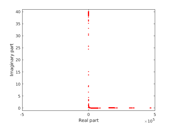
(a) Unpreconditioned

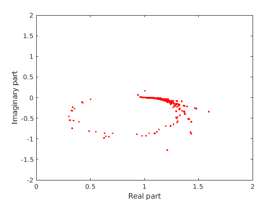
(b) Preconditioned with an homogenized coefficient

Figure 5. Spectrum of a leaf matrix of dimension $0.25\times 0.25\times 0.25$ centered at $(0.125,0.125,0.125)$ with $b(x)=-1.5e^{-160(x^{2}+y^{2}+z^{2})}$, $\kappa=40$.

Figure 5 reports on the spectrum of $\boldsymbol{A}_{\rm loc}$ without the preconditioner and the corresponding left preconditioned problem. It is clear that the preconditioner does an excellent job of clustering the spectrum at $(1,0)$. Table 1 reports the time for solving (18) via backslash in MATLAB and using the preconditioned iterative solution technique. The iterative solution technique is 19 times faster than using backslash to solve the local problem. These results illustrate the preconditioner does an excellent job efficiently handling local phenomena.

$n_{c}$	Time backslash [s]	Time iterative [s]	Speed Up
8	0.0108	0.0145	0.742
12	0.169	0.0258	6.53
16	0.815	0.0417	19.6

Table 1. Comparison of times between a direct inversion of $\boldsymbol{A}_{\rm loc}$ and a preconditioned GMRES

5. Implementation

The code for the numerical experiments in section 6 is written in FORTRAN 90. This section describes the other details about the implementation of the solution technique including hardware, compilers, libraries and related software.

5.1. Algebraic operations and sparse matrices

The Intel MKL library with complex types are utilized for the inversion of matrices, eigenvalue calculations, sparse and full matrix-matrix and matrix-vector operations. The codes are compiled using Intel FORTRAN compilers and libraries version 20.2. We use the MKL CSR format and the associated routines for algebraic operations with sparse matrices. The matrices for the leaf boxes are never constructed explicitly. The largest matrices that are constructed are the homogenized Schur complement preconditioners; $\widetilde{\boldsymbol{S}}^{\tau,-1},\forall\tau$; which are relatively small in size ($n_{b}\times n_{b}$). These homogenized Schur complement matrices are precomputed before the iterative solver is applied.

5.2. Distributed memory

The parallelization and global solvers are accessed through the PETSC library version 3.8.0. We use the KSP implementation of GMRES present in PETSC and the MatCreateShell interface for the matrix-free algorithms representing $\boldsymbol{A}$ and $\boldsymbol{J}^{-1}$. The message-passing implementation between computing nodes uses Intel MPI version $2017.0.098$.

5.3. Hardware

All experiments in Section 6, were run on the RMACC Summit supercomputer. The system has peak performance of over 400 TFLOPS. The 472 general compute nodes each have 24 cores aboard Intel Haswell CPUs, 128 GB of RAM and a local SSD. This means that each core has a limit of 4.6GB memory footprint.

All nodes are connected through a high-performance network based on Intel Omni-Path with a bandwidth of 100 GB/s and a latency of 0.4 microseconds. A 1.2 PB high-performance IBM GPFS file system is provided.

6. Numerical results

This section illustrates the performance of the solution technique presented in this paper. In all the experiments, the domain $\Omega$ is the unit cube $[0,1]^{3}$. While the variation in the medium can be any smooth function, in this paper we consider the variation in the medium $b(\boldsymbol{x})$ in (1) defined as

(19) $$b(\boldsymbol{x})=-1.5e^{-160\left((x-0.5)^{2}+(y-0.5)^{2}+(z-0.5)^{2}\right)},$$

representing a Gaussian bump centered in the middle of the unit cube. The performance of the solution technique will be similar for other choices of $b(\boldsymbol{x})$.

The Chebyshev polynomial degree is fixed with $n_{c}=16$. This follows from the two dimensional discretization versus accuracy study in [7, Section 4.1]. Also, this choice of discretization order falls into the regime where the local preconditioner was shown to be effective in section 4.2. For the scaling experiments, the solution is not known. For the experiments exploring the accuracy of the solution technique the solution is known. Throughout this section, we make reference to several different terms. For simplicity of presentation they are defined here:

$\bullet$ ppw denotes points per wavelength. The ppw are measured by counting the points along the axes and not across the diagonal of the geometry. The number of wavelengths across the diagonal of the geometry is $\sqrt{3}$ times ppw.
$\bullet$ its. denotes the number of iterations that GMRES took to achieve a specific result.
$\bullet$ Preconditioned residual reduction (PCRR) denotes the residual reduction stopping criteria set for GMRES.
$\bullet$ $r_{k}$ denotes the preconditioned residual at iteration $k$ and is defined as

$$r_{k}=\|\boldsymbol{J}^{-1}\left(\boldsymbol{b}-\boldsymbol{A}\boldsymbol{x}_{k}\right)\|_{2}$$

where $\boldsymbol{x}_{k}$ is the approximate solution at iteration $k$.
$\bullet$ The Reference Preconditioned Residual Reduction (RPRR) denotes the stopping criteria for GMRES so that all the possible digits attainable by the discretization are realized.
$\bullet$ $E_{h}$ denotes the relative error defined by

$$E_{h}=\frac{\sqrt{\displaystyle\sum_{i=1}^{N}\left(u_{h}(\boldsymbol{x}_{i})-u(\boldsymbol{x}_{i})\right)^{2}}}{\sqrt{\displaystyle\sum_{i=1}^{N}u(\boldsymbol{x}_{i})^{2}}},$$

where $N=N_{\ell}n$ is the total number of unknowns, $u_{h}(\boldsymbol{x})$ is the approximate solution at the point $\boldsymbol{x}$ obtained by allowing GMRES to run until the accuracy no longer improves, $u(\boldsymbol{x})$ is the evaluation of the exact solution at the point $\boldsymbol{x}$, and $N_{\ell}$ is the number of leaf boxes. So the $E_{h}$ will stall at the accuracy of the discretization.
$\bullet$ $E_{h}^{\rm it}$ denotes the relative error obtained by the solution created by the iterative solver when with a fixed residual reduction; i.e. stopping criterion. As the residual reduction decreases, $E_{h}^{\text{it}}$ converges to $E_{h}$.
$\bullet$ MPI Processes (MPI Procs) are the computer processes that run in parallel, exchanging information between them using the Message Passing Interface (MPI). In our paper, each core used contains only 1 MPI process and has access to a max of 4.6GB of RAM.

This section begins by illustrating the scaling of the solver. Next, section 6.2 explores the relationship between the accuracy of the solution technique and the GMRES stopping criterion in an effort to prevent from an excessive number of iterations being performed. A rule called the RPRR is developed for the stopping criterion and tested on a different problem in section 6.3.

6.1. Scaling

This section investigates the scaling of the parallel implementation of the solver. Both strong and weak scaling data is collected. Additionally, we collected data to asses the scaling of the solver for problems where the problem size in wavelengths per process is kept fixed. This last example closely aligns with how practitioners would like to solve Helmholtz problems.

For all experiments in this section, the right hand side of (1) is $s(\boldsymbol{x})=b(\boldsymbol{x})e^{i\kappa\boldsymbol{x}}$. Figure 6 illustrates the solution plotted on the planes $y=0.5$ and $z=0.5$ for $\kappa=40,\ 80,$ and $160$ with $4^{3},\ 8^{3}$, and $16^{3}$ leaves, respectively.

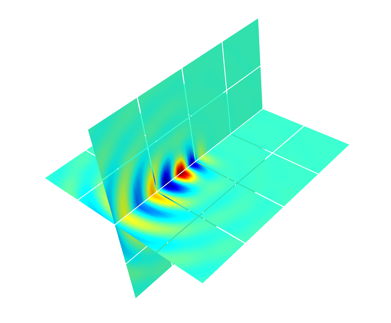
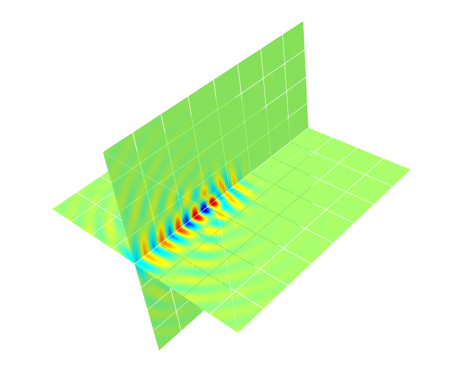
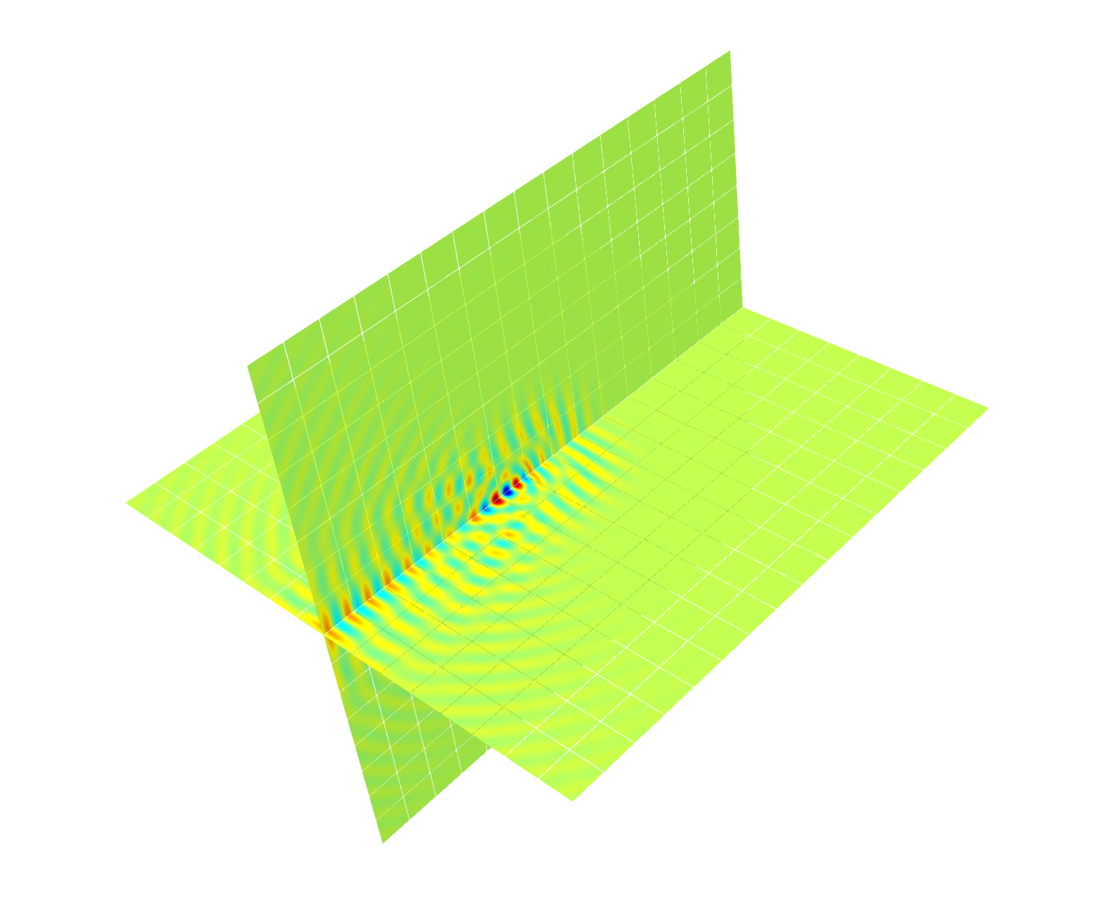
(a)	(b)	(c)

Figure 6. Illustration of the exact solution on the planes $y=0.5$ and $z=0.5$ for a problem with (a) $\kappa=40$ and $4^{3}$ leaves, (b) $\kappa=80$ and $8^{3}$ leaves, and (c) $\kappa=160$ and $16^{3}$ leaves from left to right. The $x-$axis runs diagonally to the right, the $y-$axis diagonally to the left and the $z-$axis is vertical.

6.1.1. Strong scaling

To investigate the strong scaling of the algorithm, we look at the solution time versus the number of processes for a fixed problem size. For this experiment, the stopping criterion for GMRES is fixed at $10^{-8}$. The problem under consideration is fixed with $\kappa=40$ with $8^{3}$ leaf boxes. This corresponds to the solution in Figure 6(a). The number of MPI processes gets doubled in each experiment. Figure 7 reports the scaling results. The run times reduce from approximately 7 minutes for a sequential execution to well under a minute with the minimum time happening with 16 MPI processes. The 32 MPI processes case only has 2 leaves per process, which implies that there is a lot of inter-process communication which explains the increase in time between 16 and 32 MPI processes. Even so, the solution time remains under a minute. This is thanks to the fact the purely local operations dominate the computations in this solution technique. For the other experiments, the run time approximately halves when the amount of processes is doubled which is expected from a well implemented distributed memory model.

Figure 7. A plot of the time in minutes versus the number of MPI processes when applying the presented solution technique to a problem discretized with $8^{3}$ leaf boxes to illustrate the strong scaling of the solution technique.

6.1.2. Weak scaling

Weak scaling investigates how the solution time varies with the number of processes for a fixed problem size per process and a fixed residual reduction PCRR. The discretization is refined and at the same time more MPI processes are used in order to keep the number of degrees of freedom per process constant. Two experiments are considered for weak scaling: a fixed wave number for all experiments and an increased wave number to maintain a fixed number of points per wavelength (ppw) while the mesh is refined. The latter is representative of the type of experiments desired by practitioners. Figure 8 reports the weak scaling for when the local problem size is fixed to $4^{3}$; i.e. $4^{3}$ leaf boxes are assigned to each process.

(a)	(b)

Figure 8. Illustration of the weak scaling of the algorithm. The time in minutes for solving the Helmholtz problem (a) with a fixed wave number problem with $\kappa=320$ and (b) maintaining $16$ ppw (black) and $8$ ppw (blue) on a geometry with a fixed $4\times 4\times 4$ leaves local problem on each process.

Figure 8(a) reports on the performance when the wave number fixed to $\kappa=320$ and the residual reduction is set to $10^{-10}$. The problems range from 4 to 1 a wavelength per leaf. The experiments with a small number of processes correspond to many wavelengths per leaf. For example, 64 MPI processes corresponds to 4 wavelengths per leaf while 8 MPI processes corresponds to 8 wavelengths per leaf. It is well-known that local homogenization will not work well [13] for the experiments with a high number of wavelengths per leaf. As the number of wavelengths per leaf decreases, the homogenized preconditioner performs well and the performance of the global solver is significantly better. It does reach a point where the processes are saturated and communication causes an increase in the timings.

Figure 8(b) reports on the weak scaling performance for experiments where the wave number is increased to maintain $16$ and $8$ ppw plotted in black and blue, respectively. For the $16$ ppw example, the residual reduction is fixed at $10^{-10}$ for all cases resulting is a solution that is accurate to a maximum of $8$ digits (see section 6.2). For the $8$ ppw example, the residual reduction is fixed at $10^{-8}$ for all cases resulting in a solution that is accurate to approximately $4$ digits. A flat curve is not expected in this weak scaling experiment. To understand this consider the Fourier modes of the residual. The block-Jacobi preconditioner is designed to tackle local phenomena on each leaf which corresponds to high frequency information in the residual. The lower-frequency modes in the residual remain relatively unpreconditioned. Tackling these lower-frequency modes in the residual would require a global filter, i.e. an appropriate coarse solver, which is an active area of research for Helmholtz problems. See [10, 11] for general local Fourier error analysis, [24, 23, 31] for block-Jacobi preconditioners on non-overlapping discretizations and [15, section 4] and [14] on scalable Helmholtz solvers and preconditioners.

The runtimes for the fixed number of ppw experiments grow roughly linearly for larger problems. This is expected since we use an iterative method where information is only exchanged between neighboring leaves. Necessarily, the number of steps needed to achieve a fixed residual reduction must be at least equal to the distance between opposite sides of the domain, counted in leaves sharing a face [41, p.17]. Ultimately we expect the scaling to be superlinear, but a linear behavior for regimes involving a billion degrees of freedom is very promising.

The largest problems under consideration correspond to the $4096$ MPI processes experiments in Figure 6(b) and over a billion unknowns. For the $16$ ppw example, this is a problem that is approximately $50\times 50\times 50$ wavelengths in size and it takes the solver approximately $24$ minutes to achieve the set accuracy. For the $8$ ppw example, this problem is $100\times 100\times 100$ wavelengths in size and it takes the solver approximately $17$ minutes to achieve the set accuracy. This means that by lowering the desired accuracy of the approximation, the solution technique can solve a problems twice the size in wavelengths with the same computational resources in less time.

Tables 2 and 3 report the scaling performance including the memory usage for the experiments in Figure 6(b). In these tables, it is easy to see the rough doubling of the timings and the number of iterations. It is also important to note that the increase in memory per process is low as the problem grows. This is what allowed us to solve large problems on the RMACC Summit cluster nodes which allows only 4.6 GB per process. In fact, the memory per process is under 3GB for all the experiments. This low memory footprint is thanks in large part to the exploitation of the Kronecker product structure and the sparsity of operators.

Problem size in leaves	$4\times 4\times 4$	$8\times 8\times 8$	$16\times 16\times 16$	$32\times 32\times 32$	$64\times 64\times 64$
Problem size in wavelengths	$3$	$6$	$12$	$24$	$48$
MPI procs	1	8	64	512	4096
Degrees of freedom $N$	250k	2M	16M	128M	1027M
GMRES iterations	156	216	402	736	1478
GMRES time	28s	61s	122s	541s	1444s
Peak memory per process	1.94 GB	2.21 GB	2.29GB	2.38 GB	2.70 GB

Table 2. Problem size in wavelengths, MPI processes (MPI procs), number of discretization points, number of GMRES iterations, time for the iterative solver to converge with a preconditioned relative residual of $10^{-10}$, and the peak memory per process for different problem sizes. Here the wave number is increased to maintain $16$ ppw.

Problem size in leaves	$4\times 4\times 4$	$8\times 8\times 8$	$16\times 16\times 16$	$32\times 32\times 32$	$64\times 64\times 64$
Problem size in wavelengths	$6$	$12$	$24$	$48$	$96$
MPI procs	1	8	64	512	4096
Degrees of freedom $N$	250k	2M	16M	128M	1027M
GMRES iterations	153	191	315	567	1065
GMRES time	30s	54s	95s	209s	1055s
Peak memory per process	1.92 GB	2.21 GB	2.29GB	2.37 GB	2.70 GB

Table 3. Problem size in wavelengths, MPI processes (MPI procs), number of discretization points, number of GMRES iterations, time for the iterative solver to converge with a preconditioned relative residual of $10^{-8}$, and the peak memory per process for different problem sizes. Here the wave number is increased to maintain $8$ ppw.

6.2. Relative residual rule for maximum accuracy

This section investigates the necessary stopping criterion for GMRES in order to guarantee that all the digits that are achievable by the discretization. To do this, we consider the boundary value problem with an exact solution of

(20) $$u(x,y,z)=e^{i\kappa(x+y+z)}e^{x}\cosh(y)(z+1)^{2}$$

for different wave numbers $\kappa$ and the variable coefficient $b(\boldsymbol{x})$ as defined in equation (19). Figure 9 illustrates the solution for different values of $\kappa$. The exact solution (20) is a plane wave in the direction $(1,1,1)$ that is modulated differently along the $x$, $y$ and $z$ axes.

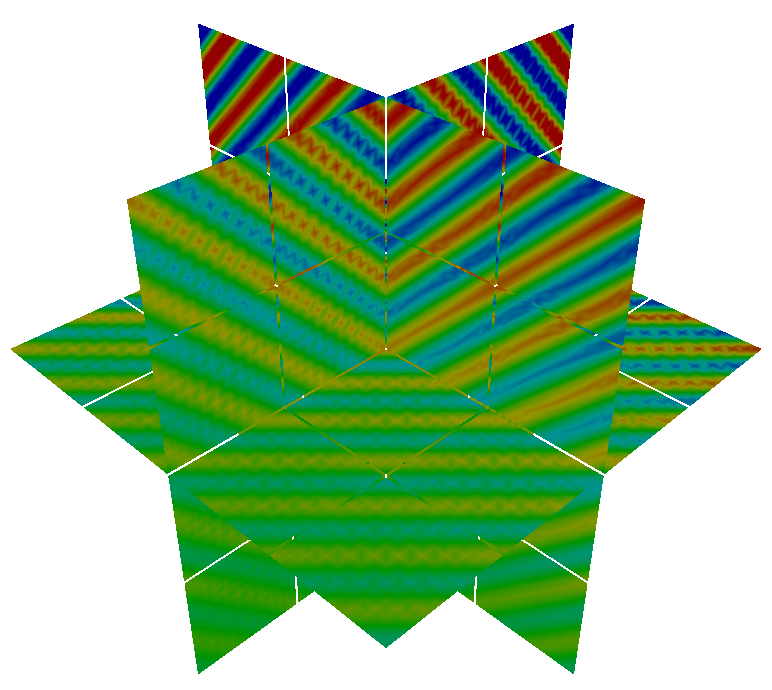
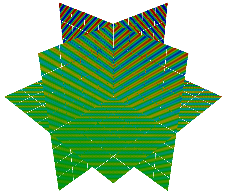
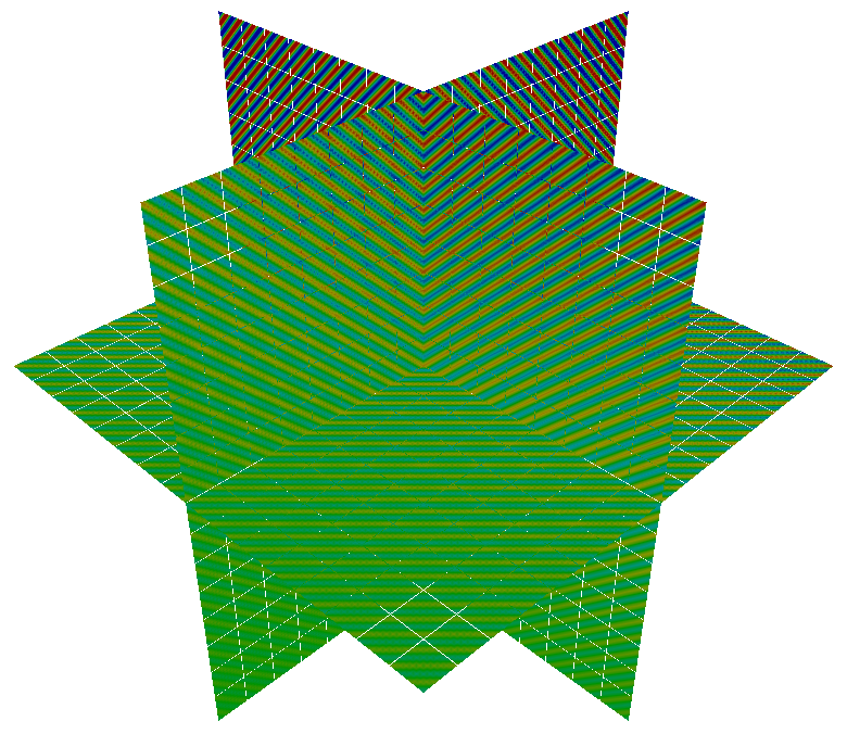
(a)	(b)	(c)

Figure 9. Illustration of the exact solution (20) when $9.6$ ppw is maintained for $4^{3}$, $8^{3}$ and $16^{3}$ leaves (from left to right). The plots of the solution are on the planes $x=0.5$, $y=0.5$ and $z=0.5$ where the $x-$axis runs diagonally to the right, the $y-$axis diagonally to the left and the $z-$axis is vertical.

Table 4 reports the relative error $E_{h}$ and digits of accuracy obtained by the discretization when the number of ppw remains fixed across a row. The error $E_{h}$ related to the ppw remains fixed. This is consistent with the accuracy observed when applying this discretization to two dimensional problems. The values range from orders of magnitude of $10^{-12}$ for 24 ppw to $10^{-7}$ for 9.6 ppw.

Table 4. The relative error $E_{h}$ and number of digits of accuracy obtained for different ppw and number of leaf boxes for the problem considered in section 6.2 .

	$4^{3}$	$8^{3}$	$16^{3}$	$32^{3}$	Digits
24.0	2.057E-12	1.763E-12	1.715E-12	1.727E-12	11
19.2	8.872E-11	9.166E-11	9.275E-11	9.360E-11	10
16.0	1.514E-09	1.922E-09	1.631E-09	1.667E-09	8
12.0	7.121E-08	7.246E-08	7.221E-08	7.313E-08	7
9.60	6.932E-07	5.631E-07	4.836E-07	4.478E-07	6

By looking at the residual reduction at each iteration of GMRES we are able to define a stopping criterion which prevents extra iterations from being performed but the accuracy of the discretization is achieved. As defined in the beginning of section 6, we call this the RPRR. Table 5 reports the RPRR and the corresponding relative iterative error $E_{h}^{\text{it}}$ when using this stopping criterion for the same problems as in Table 4. The relative errors reported in both tables match in terms of digits.

Table 6 reports the time in seconds for the solver and the number of GMRES iterations needed to obtain the residual reduction in Table 5. The results from this section suggest that it is sufficient to ask for the residual reduction to be about two digits smaller than the expected accuracy of the discretization. Another observation from Table 6 is that while the problem at 9.60 ppw has a solution that is more oscillatory than the problem at 24 ppw the solution technique converges faster. This is because a lower accuracy solution is obtained and the stopping criterion for GMRES is also lower. Looking left-to-right in this table, the number of iterations and time to convergence increases. This is due to the global problem becoming larger in number of wavelengths as the number of leaf boxes increases and the need to propagate information across all the boxes.

Table 5. The RPRR needed to guarantee that the accuracy of the discretization is achieved in for the experiments in Table 4. The relative error $E_{h}^{\text{it}}$ is reported when using the RPRR as the stopping criteria for GMRES.

	$4^{3}$	$8^{3}$	$16^{3}$	$32^{3}$	RPRR
24.0	8.122E-13	1.632E-12	8.844E-13	5.231E-13	$10^{-13}$
19.2	8.883E-12	6.632E-12	3.534E-12	1.917E-12	$10^{-12}$
16.0	1.275E-09	1.681E-09	1.021E-09	5.151E-10	$10^{-10}$
12.0	1.438E-08	1.145E-08	7.215E-09	3.326E-09	$10^{-9}$
9.60	2.541E-07	1.385E-07	8.280E-08	4.408E-08	$10^{-8}$

Table 6. The time in seconds it takes GMRES and number of iterations it takes GMRES to converge with the RPRR as the stopping criterion from table 5 for various points per wavelength and meshes.

	$4^{3}$		$8^{3}$		$16^{3}$		$32^{3}$
	time[s]	its.	time[s]	its.	time[s]	its.	time[s]	its.
24.0	48	216	97	296	351	477	947	775
19.2	55	187	125	263	278	392	869	668
16.0	35	146	96	184	389	277	482	466
12.0	40	141	78	165	281	243	554	407
9.6	38	140	38	142	235	191	447	320

6.3. Effectiveness of the proposed rule for stopping criteria

This section verifies the effectiveness of the RPRR proposed in section 6.2 as the stopping criteria for GMRES. That is, the desired residual reduction is set to 2-3 digits more than the accuracy that can be achieved by the discretization.

The experiments in this section have an exact solution given by

(21) $$u(x,y,z)=\left(1+e^{i\kappa x}\right)\left(1+e^{i\kappa y}\right)\left(1+e^{i\kappa z}\right)\ln\left(1+x^{2}+y^{2}+z^{2}\right)$$

which is not separable. The variable coefficient $b(\boldsymbol{x})$ is defined in equation (19). Figure 10 illustrates the solution (21) for different values of $\kappa$. Roughly speaking, it is a grid of bumps along any axis that is modulated by the function $\ln\left(1+x^{2}+y^{2}+z^{2}\right)$. The pattern of bumps makes it easy to observe the number of wavelengths along the axes. Given that this solution is more oscillatory (with roughly the same magnitude) throughout the geometry than the solution in the previous section, it is expected that it will take more iterations for GMRES to converge. This is especially true for high frequency problems.

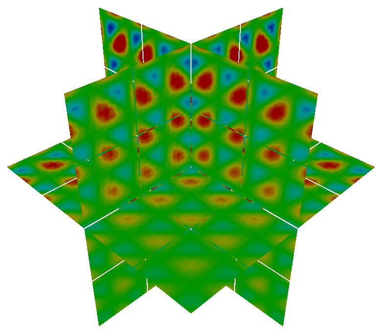
(a)	(b)	(c)

Figure 10. Illustration of the bumps solution (21) cut at the planes $x=0.5$, $y=0.5$ and $z=0.5$ for $9.6$ ppw with discretizations consisting of (a) $4^{3}$, (b) $8^{3}$ and (c) $16^{3}$ leaves. The $x-$axis runs diagonally to the right, the $y-$axis diagonally to the left and the $z-$axis is vertical.

Table 7 reports the relative error $E_{h}^{\text{it}}$ obtained by using the relative residual stopping criteria prescribed in the Section 6.2. The orders of magnitude in the error are similar to what was observed for the separable solution in Table 4 confirming the accuracy of the discretization. Table 8 reports the maximum achievable accuracy of the discretization $E_{h}$. The two errors are of the same order. This means that the stopping criteria is giving the maximum possible accuracy attainable by the discretization.

Table 7. The relative error $E_{h}^{\text{it}}$ obtained for different ppw and discretizations using the RPRR rule for the boundary value problem with solution given in (21).

	$4^{3}$	$8^{3}$	$16^{3}$	$32^{3}$
24.0	3.647E-12	3.957E-12	6.770E-12	1.270E-11
19.2	1.456E-10	2.933E-10	5.432E-10	1.004E-09
16.0	2.930E-09	7.184E-09	1.377E-08	2.869E-08
12.0	1.528E-07	2.629E-07	4.573E-07	7.196E-07
9.60	5.389E-06	1.614E-06	2.857E-06	4.461E-06

Table 8. The relative error $E_{h}$ obtained for different ppw and discretizations for the boundary value problem with solution (21). Here GMRES was allowed to run until it the residual reduction was machine precision.

	$4^{3}$	$8^{3}$	$16^{3}$	$32^{3}$
24.0	3.738E-12	3.856E-12	6.736E-12	1.263E-11
19.2	1.480E-10	3.035E-10	5.432E-10	1.004E-09
16.0	2.910E-09	6.588E-09	1.376E-08	2.861E-08
12.0	1.528E-07	2.630E-07	4.573E-07	7.197E-07
9.60	1.302E-06	1.614E-06	2.856E-06	4.458E-06

Table 9 reports the times and number of iterations needed for GMRES to converge with the prescribed residual reduction. As expected, since the solution to the problem in this section is more oscillatory than in the previous section, more iterations are needed to achieve the same accuracy with the same discretizations. All other trends observed in the experiments from section 6.2 remain the same.

Table 9. The time in seconds and number of iterations needed for GMRES to achieve maximum accuracy using the RPRR rule for the boundary value problem with solution (21.

	$4^{3}$		$8^{3}$		$16^{3}$		$32^{3}$
	time[s]	its.	time[s]	its.	time[s]	its.	time[s]	its.
24.0	58	242	90	352	493	559	969	948
19.2	42	205	112	288	281	456	929	827
16.0	39	170	92	236	205	379	702	663
12.0	60	168	80	201	163	320	610	557
9.6	75	163	138	190	310	280	531	480

7. Concluding remarks

This manuscript presented an efficient iterative solution technique for the linear system that results from the HPS discretization of variable coefficient Helmholtz problems. The technique is based on a block-Jacobi preconditioner coupled with GMRES. The preconditioner is based on local homogenization and is extremely efficient to apply thanks to the tensor product nature of the discretization. The homogenization is highly effective because the elements (or leaves) are never many wavelengths in size.

The numerical results illustrate the effectiveness of the solution technique. While the method does not “scale” in the parallel computing context, it is extremely efficient. For example, it is able to solve a three dimensional mid frequency Helmholtz problem (roughly 100 wavelengths in each direction) requiring over 1 billion discretization points to achieve approximately 4 digits of accuracy in under 20 minutes on a cluster. The numerical results also illustrate that the HPS method is able to achieve a prescribed accuracy at set ppw. This is consistent with the accuracy observed for two dimensional problem [7, 18]. Additionally, the numerical results indicate that it is sufficient to ask for the relative residual of approximately 2-3 digits more than the accuracy expected of the discretization. This will minimize the number of extra iterations performed by GMRES but does not effect the accuracy of the solution technique.

As mentioned in the text, the proposed solver does not scale. In future work, one could develop a multi-level solver where the block-Jacobi preconditioner will be used as smoother between the coarse and the fine grids. Efficient solvers for the coarse grid is ongoing work.

References

- [1] Ivo Babuška, Frank Ihlenburg, Ellen T. Paik, and Stefan A. Sauter, A generalized finite element method for solving the Helmholtz equation in two dimensions with minimal pollution, Computer Methods in Applied Mechanics and Engineering 128 (1995), no. 3, 325–359.
- [2] Ivo M. Babuška and Stefan A. Sauter, Is the pollution effect of the fem avoidable for the Helmholtz equation considering high wave numbers?, SIAM Journal on Numerical Analysis 34 (1997), no. 6, 2392–2423.
- [3] Satish Balay, Shrirang Abhyankar, Mark F. Adams, Jed Brown, Peter Brune, Kris Buschelman, Lisandro Dalcin, Alp Dener, Victor Eijkhout, William D. Gropp, Dmitry Karpeyev, Dinesh Kaushik, Matthew G. Knepley, Dave A. May, Lois Curfman McInnes, Richard Tran Mills, Todd Munson, Karl Rupp, Patrick Sanan, Barry F. Smith, Stefano Zampini, Hong Zhang, and Hong Zhang, PETSc users manual, Tech. Report ANL-95/11 - Revision 3.15, Argonne National Laboratory, 2021.
- [4] by same author, PETSc Web page, https://www.mcs.anl.gov/petsc, 2021.
- [5] Satish Balay, William D. Gropp, Lois Curfman McInnes, and Barry F. Smith, Efficient management of parallelism in object oriented numerical software libraries, Modern Software Tools in Scientific Computing (E. Arge, A. M. Bruaset, and H. P. Langtangen, eds.), Birkhäuser Press, 1997, pp. 163–202.
- [6] A. Bayliss, C.I. Goldstein, and E. Turkel, On accuracy conditions for the numerical computation of waves, Journal of Computational Physics 59 (1985), no. 3, 396–404.
- [7] Natalie N. Beams, Adrianna Gillman, and Russell J. Hewett, A parallel shared-memory implementation of a high-order accurate solution technique for variable coefficient Helmholtz problems, Computers & Mathematics with Applications 79 (2020), no. 4, 996–1011.
- [8] Thomas Beck, Yaiza Canzani, and Jeremy L. Marzuola, Quantitative bounds on impedance-to-impedance operators with applications to fast direct solvers for PDEs, 2021.
- [9] J. Boyd, Chebyshev and fourier spectral methods, 2nd ed., Dover, Mineola, New York, 2001.
- [10] Achi Brandt, Multi-level adaptive solutions to boundary-value problems, Mathematics of Computation 31 (1977), no. 138, 333–390.
- [11] by same author, Rigorous quantitative analysis of multigrid. i. constant coefficients two-level cycle with -norm, SIAM J. Numer. Anal. 6 (1994), no. 31, 1695–1730.
- [12] S. N. Chandler-Wilde, The impedance boundary value problem for the helmholtz equation in a half-plane, Mathematical Methods in the Applied Sciences 20 (1997), no. 10, 813–840.
- [13] Théophile Chaumont Frelet, Finite element approximation of Helmholtz problems with application to seismic wave propagation, Theses, INSA de Rouen, Dec 2015.
- [14] O. G. Ernst and M. J. Gander, Why it is difficult to solve helmholtz problems with classical iterative methods, pp. 325–363, Springer Berlin Heidelberg, Berlin, Heidelberg, 2012.
- [15] Martin J. Gander and Hui Zhang, A class of iterative solvers for the helmholtz equation: Factorizations, sweeping preconditioners, source transfer, single layer potentials, polarized traces, and optimized schwarz methods, SIAM Review 61 (2019), no. 1, 3–76.
- [16] P. Geldermans and A. Gillman, An adaptive high order direct solution technique for elliptic boundary value problems, SIAM Journal on Scientific Computing 41 (2019), no. 1, A292–A315.
- [17] Alan George, Nested dissection of a regular finite element mesh, SIAM Journal on Numerical Analysis 10 (1973), no. 2, 345–363.
- [18] A. Gillman, A. H. Barnett, and P-G. Martinsson, A spectrally accurate direct solution technique for frequency-domain scattering problems with variable media, BIT Numerical Mathematics 55 (2015), no. 1, 141–170.
- [19] A. Gillman and P. G. Martinsson, A direct solver with $o(n)$ complexity for variable coefficient elliptic PDEs discretized via a high-order composite spectral collocation method, SIAM Journal on Scientific Computing 36 (2014), no. 4, A2023–A2046.
- [20] I. G. Graham and S. A. Sauter, Stability and finite element error analysis for the helmholtz equation with variable coefficients, Mathematics of Computation 89 (2020), 105–138.
- [21] X. Pinel H. Calandra, S. Gratton and X. Vasseur, An improved two-grid preconditioner for the solution of three-dimensional helmholtz problems in heterogeneous media, Numer. Linear Algebra Appl. 20 (2012), 663–688.
- [22] Sijia Hao and Per-Gunnar Martinsson, A direct solver for elliptic PDEs in three dimensions based on hierarchical merging of Poincaré–Steklov operators, Journal of Computational and Applied Mathematics 308 (2016), 419–434.
- [23] P. Hemker, W. Hoffmann, and M. van Raalte, Two-level fourier analysis of a multigrid approach for discontinuous Galerkin discretization, SIAM Journal on Scientific Computing 3 (2003), no. 25, 1018–1041.
- [24] P. W. Hemker, W. Hoffmann, and M. H. van Raalte, Fourier two-level analysis for discontinuous Galerkin discretization with linear elements, Numerical Linear Algebra with Applications 5 – 6 (2004), no. 11, 473–491.
- [25] Lighthill M. J., Waves in fluids, Cambridge University Press, Cambridge, England, 1978.
- [26] S. Kim and M. Lee, Artificial damping techniques for scalar waves in the frequency domain, Comput. Math. Appl. 31 (1996), 1–12.
- [27] L. E. Kinsler, A. R. Frey, A. B. Coppens, and J. V. Sanders., Fundamentals of acoustics, Wiley, 2000.
- [28] Andrew V. Knyazev, Toward the optimal preconditioned eigensolver: Locally optimal block preconditioned conjugate gradient method, SIAM Journal on Scientific Computing 23 (2001), no. 2, 517–541.
- [29] Martin Kronbichler and Katharina Kormann, Fast matrix-free evaluation of discontinuous galerkin finite element operators, ACM Trans. Math. Softw. 45 (2019), no. 3.
- [30] Alexander G. Kyurkchan and Nadezhda I. Smirnova, Mathematical modeling in diffraction theory, Elsevier, Amsterdam, 2016.
- [31] José Pablo Lucero Lorca and Martin Jakob Gander, Optimization of two-level methods for dg discretizations of reaction-diffusion equations, 2020.
- [32] P.G. Martinsson, A fast direct solver for a class of elliptic partial differential equations, Journal of Computational Physics 38 (2009), 316–330.
- [33] by same author, A direct solver for variable coefficient elliptic PDEs discretized via a composite spectral collocation method, Journal of Computational Physics 242 (2013), 460–479.
- [34] H.P. Pfeiffer, L.E. Kidder, M.A. Scheel, and S.A. Teukolsky, A multidomain spectral method for solving elliptic equations, Computer physics communications 152 (2003), no. 3, 253–273.
- [35] C. D. Riyanti, A. Kononov, Y. A. Erlangga, C. Vuik, C. W. Oosterlee, R.-E. Plessix, and W. A. Mulder, A parallel multigrid-based preconditioner for the 3d heterogeneous high-frequency helmholtz equation, J. Comput. Phys. 224 (2007), 431–448.
- [36] W. E. Roth, On direct product matrices, Bulletin of the American Mathematical Society 40 (1934), no. 6, 461 – 468.
- [37] B. Reps S. Cools and W. Vanroose, A new level-dependent coarse grid correction scheme for indefinite helmholtz problems, Numer. Linear Algebra Appl. 21 (2014), 513–533.
- [38] Youcef Saad and Martin H. Schultz, GMRES: A generalized minimal residual algorithm for solving nonsymmetric linear systems, SIAM Journal on Scientific and Statistical Computing 7 (1986), no. 3, 856–869.
- [39] Enrique Sanchez-Palencia, Non-homogeneous media and vibration theory, Lecture Notes in Physics, Springer-Verlag, Berlin, Heidelberg, 1980.
- [40] Barry Francis Smith, Petter E. Bjørstad, and William D. Gropp, Domain decomposition : parallel multilevel methods for elliptic partial differential equations, Cambridge University Press, Cambridge, 1996.
- [41] Andrea Toselli and Olof B. Widlund, Domain decomposition methods : algorithms and theory, Springer series in computational mathematics, Springer, Berlin, 2005.
- [42] Lloyd N. Trefethen, Spectral methods in matlab, Society for Industrial and Applied Mathematics, 2000.
- [43] C. Vuik Y. A. Erlangga and C. W. Oosterlee, On a class of preconditioners for the helmholtz equation, Appl. Numer. Math. 50 (2004), 409–425.