Behind the Curtain: Learning Occluded Shapes for 3D Object Detection

Abstract

Advances in LiDAR sensors provide rich 3D data that supports 3D scene understanding. However, due to occlusion and signal miss, LiDAR point clouds are in practice 2.5D as they cover only partial underlying shapes, which poses a fundamental challenge to 3D perception. To tackle the challenge, we present a novel LiDAR-based 3D object detection model, dubbed Behind the Curtain Detector (BtcDet), which learns the object shape priors and estimates the complete object shapes that are partially occluded (curtained) in point clouds. BtcDet first identifies the regions that are affected by occlusion and signal miss. In these regions, our model predicts the probability of occupancy that indicates if a region contains object shapes. Integrated with this probability map, BtcDet can generate high-quality 3D proposals. Finally, the probability of occupancy is also integrated into a proposal refinement module to generate the final bounding boxes. Extensive experiments on the KITTI Dataset (Geiger et al. 2013) and the Waymo Open Dataset (Sun et al. 2019) demonstrate the effectiveness of BtcDet. Particularly, for the 3D detection of both cars and cyclists on the KITTI benchmark, BtcDet surpasses all of the published state-of-the-art methods by remarkable margins. Code is released .

1 Introduction

Figure 1: The impact of the three types of shape miss. (b) shows PV-RCNN’s (Shi et al. 2020) car 3D detection APs with different occlusion levels on the KITTI (Geiger et al. 2013) val split. NR means no shape miss recovery. EO, SM, and SO indicate adding car points in the regions of external-occlusion, signal miss and self-occlusion, respectively, as visualized in (a).

With high-fidelity, the point clouds acquired by LiDAR sensors significantly improved autonomous agents’s ability to understand 3D scenes. LiDAR-based models achieved state-of-the-art performance on 3D object classification (Xu et al. 2020), visual odometry (Pan et al. 2021), and 3D object detection (Shi et al. 2020). Despite being widely used in these 3D applications, LiDAR frames are technically 2.5D. After hitting the first object, a laser beam will return and leave the shapes behind the occluder missing from the point cloud.

To locate a severely occluded object (e.g., the car in Figure LABEL:fig:teaser(b)), a detector has to recognize the underlying object shapes even when most of its parts are missing. Since shape miss inevitably affects object perception, it is important to answer two questions:

• What are the causes of shape miss in point clouds?

• What is the impact of shape miss on 3D object detection?

1.1 Causes of Shape Miss

To answer the first question, we study the objects in KITTI (Geiger et al. 2013) and discover three causes of shape miss.

External-occlusion. As visualized in Figure LABEL:fig:teaser(c), occluders block the laser beams from reaching the red frustums behind them. In this situation, the external-occlusion is formed, which causes the shape miss located at the red voxels.

Signal miss. As Figure LABEL:fig:teaser(c) illustrates, certain materials and reflection angles prevent laser beams from returning to the sensor after hitting some regions of the car (blue voxels). After projected to range view, the affected blue frustums in Figure LABEL:fig:teaser(c) appear as the empty pixels in Figure LABEL:fig:teaser(a).

Self-occlusion. LiDAR data is 2.5D by nature. As shown in Figure LABEL:fig:teaser(d), for a same object, its parts on the far side (the green voxels) are occluded by the parts on the near side. The shape miss resulting from self-occlusion inevitably happens to every object in LiDAR scans.

1.2 Impact of Shape Miss

To analyze the impact of shape miss on 3D object detection, we evaluate the car detection results of the scenarios where we recover certain types of shape miss on each object by borrowing points from similar objects (see the details of finding similar objects and filling points in Sec. 3.1).

In each scenario, after resolving certain shape miss in both the train and val split of KITTI (Geiger et al. 2013), we train and evaluate a popular detector PV-RCNN (Shi et al. 2020). The four scenarios are:

• NR: Using the original data without shape miss recovery.

• EO: Recovering the shape miss caused by external-occlusion (adding the red points in Figure 1(a)).

• EO+SM: Recovering the shape miss caused by external-occlusion and signal miss (adding the red and blue points in Figure 1(a)).

• EO+SM+SO: Recovering all the shape miss (adding the red, blue and green points in Figure 1(a)).

We report detection results on cars with three occlusion levels (level labels are provided by the dataset). As shown in Figure 1(b), without recovery (NR), it is more difficult to detect objects with higher occlusion levels. Recovering shapes miss will reduce the performance gaps between objects with different levels of occlusion . If all shape miss are resolved (EO+SM+SO), the performance gaps are eliminated and almost all objects can be effectively detected (APs $>$ $99\%$).

1.3 The Proposed Method

The above experiment manually resolves the shape miss by filling points into the labeled bounding boxes and significantly improve the detection results. However, during test time, how do we resolve shape miss without knowing bounding box labels?

In this paper, we propose Behind the Curtain Detector (BtcDet). To the best of our knowledge, BtcDet is the first 3D object detector that targets the object shapes affected by occlusion. With the knowledge of shape priors, BtcDet estimates the occupancy of complete object shapes in the regions affected by occlusion and signal miss. After being integrated into the detection pipeline, the occupancy estimation benefits both region proposal generation and proposal refinement. Eventually, BtcDet surpasses all of the state-of-the-art methods published to date by remarkable margins.

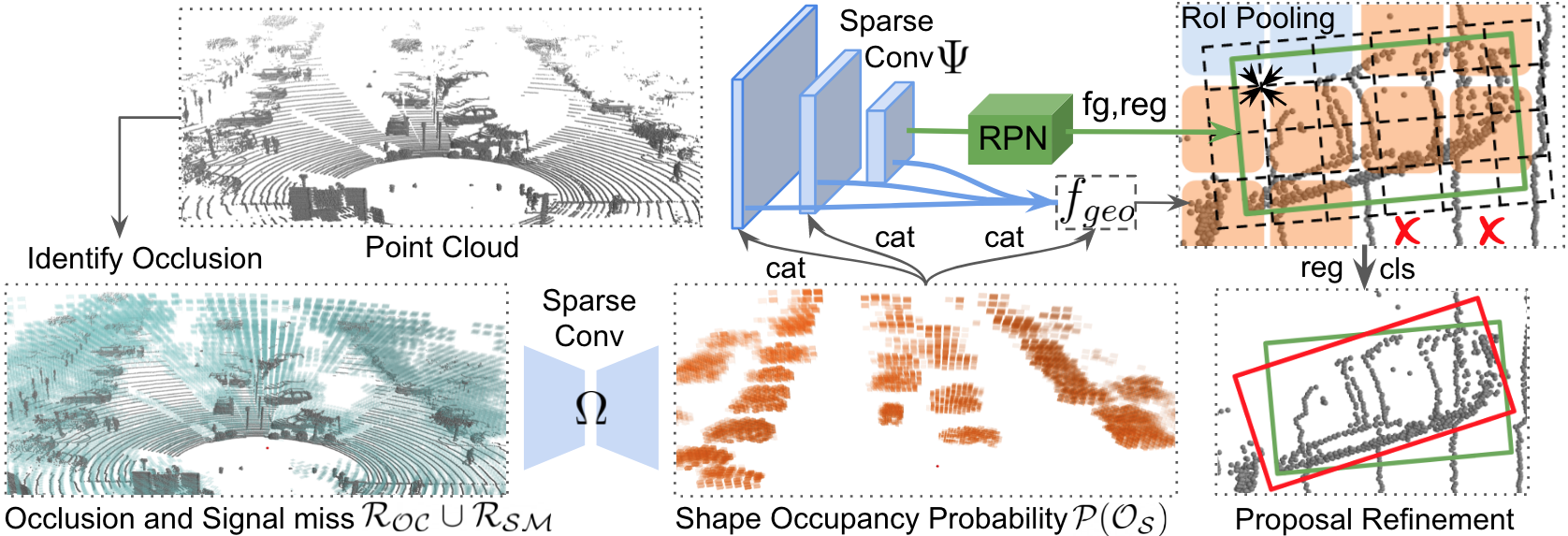
Figure 2: The detection pipeline. BtcDet first identifies the regions of occlusion and signal miss $\mathcal{R_{OC}}\cup\mathcal{R_{SM}}$İn these regions, BtcDet estimates the shape occupancy probability $\mathcal{P}(\mathcal{O_{S}})$ (the orangex voxels have $\mathcal{P}(\mathcal{O_{S}})$ $>0.3$). When the backbone network $\Psi$ extracts detection features from the point cloud, $\mathcal{P}(\mathcal{O_{S}})$ is concatenated with $\Psi$’s intermediate feature maps. Then, a RPN network takes the output and generates 3D proposals. For each proposal (e.g., the green box), BtcDet pools the local geometric features $f_{geo}$ to the nearby grids and finally generate the final bounding box prediction (the red box) and the confidence score.

2 Related Work

LiDAR-based 3D object detectors. Voxel-based methods divide point clouds by voxel grids to extract features (Zhou and Tuzel 2018). Some of them also use sparse convolution to improve model efficiency, e.g., SECOND(Yan et al. 2018). Point-based methods such as PointRCNN (Shi et al. 2019a) generate proposals directly from points. STD (Yang et al. 2019) applies sparse to dense refinement and VoteNet (Qi et al. 2019a) votes the proposal centers from point clusters. These models are supervised on the ground truth bounding boxes without explicit consideration for the object shapes.

Learning shapes for 3D object detection. Bounding box prediction requires models to understand object shapes. Some detectors learn the shape related statistics as an auxiliary task. PartA² (Shi et al. 2020) learns object part locations. SA-SSD and AssociateDet (He et al. 2020; Du et al. 2020) use auxiliary networks to preserve structural information. Studies (Li et al. 2021; Yan et al. 2020; Najibi et al. 2020; Xu et al. 2021) such as SPG conduct point cloud completion to improve object detection. These models are shape-aware but overlook the impact of occlusion on object shapes.

Occlusion handling in computer vision. The negative impact of occlusion on various computer vision tasks, including tracking (Liu et al. 2018), image-based pedestrian detection (Zhang et al. 2018), image-based car detection (Reddy et al. 2019) and semantic part detection (Saleh et al. 2021), is acknowledged. Efforts addressing occlusion include the amodal instance segmentation (Follmann et al. 2019), the Multi-Level Coding that predicts the presence of occlusion (Qi et al. 2019b). These studies, although focus on 2D images, demonstrate the benefits of modeling occlusion to solving visual tasks. Point cloud visibility is addressed in (Hu et al. 2020) and is used in multi-frame detection and data augmentation. This method, however, does not learn and explore the visibility’s influence on object shapes. Our proposed BtcDet is the first 3D object detector that learns occluded shapes in point cloud data. We compare (Hu et al. 2020)’s approach with ours in Sec. 4.3.

3 Behind the Curtain Detector

Let $\Theta$ denote the parameters of a detector, $\{p_{1},p_{2},...,p_{N}\}$ denote the LiDAR point cloud, $\mathcal{X},\mathcal{D},{\mathcal{S}_{ob}},{\mathcal{S}_{oc}}$ denote the estimated box center, the box dimension, the observed objects shapes and the occluded object shapes, respectively. Most LiDAR-based 3D object detectors (Yi et al. 2020; Chen et al. 2020; Shi and Rajkumar 2020) only supervise the bounding box prediction. These models have

$$\Theta_{MLE}=\operatorname*{argmax}_{\Theta}P(\mathcal{X},\mathcal{D}\ |\ \{p_{1},p_{2},...,p_{N}\},\Theta),$$ (1)

while structure-aware models (Shi et al. 2020; He et al. 2020; Du et al. 2020) also supervise ${\mathcal{S}_{ob}}$’s statistics so that

$$\Theta_{MLE}=\operatorname*{argmax}_{\Theta}P(\mathcal{X},\mathcal{D},\mathcal{S}_{ob}\ |\ \{p_{1},p_{2},...,p_{N}\},\Theta).$$ (2)

None of the above studies explicitly model the complete object shapes $\mathcal{S}=\mathcal{S}_{ob}\cup\mathcal{S}_{oc}$, while the experiments in Sec. 1.2 show the improvements if $\mathcal{S}$ is obtained. BtcDet estimates $\mathcal{S}$ by predicting the shape occupancy $\mathcal{O_{S}}$ for regions of interest. After that, BtcDet conducts object detection conditioned on the estimated probability of occupancy $\mathcal{P}(\mathcal{O_{S}})$. The optimization objectives can be described as follows:

$$\operatorname*{argmax}_{\Theta}P(\mathcal{O_{S}}\ |\ \{p_{1},p_{2},...,p_{N}\},\mathcal{R_{SM}},\mathcal{R_{OC}},\Theta),$$ (3)

$$\operatorname*{argmax}_{\Theta}P(\mathcal{X},\mathcal{D}\ |\ \{p_{1},p_{2},...,p_{N}\},\mathcal{P}(\mathcal{O_{S}}),\Theta).$$ (4)

Model overview. As illustrated in Figure 2, BtcDet first identifies the regions of occlusion $\mathcal{R_{OC}}$ and signal miss $\mathcal{R_{SM}}$, and then, let a shape occupancy network $\Omega$ estimate the probability of object shape occupancy $\mathcal{P}(\mathcal{O_{S}})$. The training process is described in Sec. 3.1.

Next, BtcDet extracts the point cloud 3D features by a backbone network $\Psi$. The features are sent to a Region Proposal Network (RPN) to generate 3D proposals. To leverage the occupancy estimation, the sparse tensor $\mathcal{P}(\mathcal{O_{S}})$ is concatenated with the feature maps of $\Psi$. (See Sec. 3.2.)

Finally, BtcDet applies the proposal refinement. The local geometric features $f_{geo}$ are composed of $\mathcal{P}(\mathcal{O_{S}})$ and the multi-scale features from $\Psi$. For each region proposal, we construct local grids covering the proposal box. BtcDet pools the local geometric features $f_{geo}$ onto the local grids, aggregates the grid features, and generates the final bounding box predictions. (See Sec. 3.3.)

3.1 Learning Shapes in Occlusion

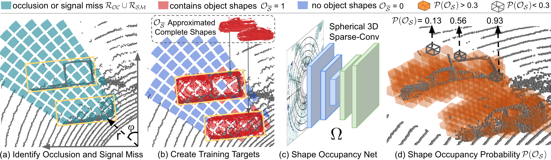
Figure 3: Learning Occluded Shapes. (a) The regions of occlusion or signal miss $\mathcal{R_{OC}}\cup\mathcal{R_{SM}}$ can be identified after the spherical voxelization for the point cloud. (b) To label the occupancy $\mathcal{O_{\overline{S}}}$ (1 or 0), We place the approximated complete object shapes $\overline{S}$ (red points) in the corresponding boxes. (c) A shape occupancy network $\Omega$ predicts the shape occupancy probability $\mathcal{P}(\mathcal{O_{S}})$ for voxels in $\mathcal{R_{OC}}\cup\mathcal{R_{SM}}$ , supervised by $\mathcal{O_{\overline{S}}}$. (d) Voxels are colored orange if it has a prediction $\mathcal{P}(\mathcal{O_{S}})$ $>0.3$.

Approximate the complete object shapes for ground truth labels. Occlusion and signal miss preclude the knowledge of the complete object shapes $S$. However, we can assemble the approximated complete shapes $\overline{\mathcal{S}}$, based on two assumptions:

• Most foreground objects resemble a limited number of shape prototypes, e.g., pedestrians share a few body types.

• Foreground objects, especially vehicles and cyclists, are roughly symmetric.

We use the labeled bounding boxes to query points belonging to the objects. For cars and cyclists, we mirror the object points against the middle section plane of the bounding box.

A heuristic $\mathcal{H}(A,B)$ is created to evaluate if a source object $B$ covers most parts of a target object $A$ and provides points that can fill $A$’s shape miss. To approximate $A$’s complete shape, we select the top 3 source objects $B_{1},B_{2},B_{3}$ with the best scores. The final approximation $\overline{\mathcal{S}}$ consists of $A$’s original points and the points of $B_{1},B_{2},B_{3}$ that fill $A$’s shape miss. The target objects are the occluded object in the current training frame, while the source objects are other objects of the same class in the detection training set. Both can be extracted by the ground truth bounding boxes. Please find details of $\mathcal{H}(A,B)$ in Appendix B and more visualization of assembling $\overline{\mathcal{S}}$ in Appendix G.

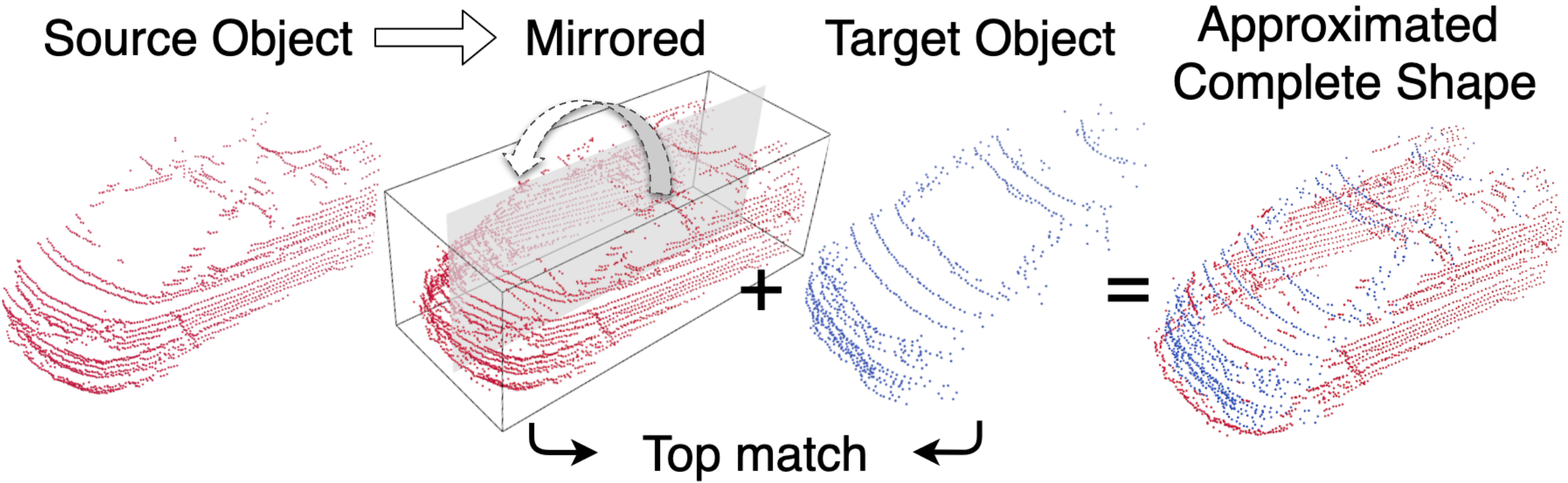
Figure 4: Assemble the approximated complete shape $\overline{\mathcal{S}}$ for an object (blue) by using points from top match objects.

Identify $\mathcal{R_{OC}}\cup\mathcal{R_{SM}}$ in the spherical coordinate system. According to our analysis in Sec. 1.1, “shape miss” only exists in the occluded regions $\mathcal{R_{OC}}$ and the regions with signal miss $\mathcal{R_{SM}}$ (see Figure LABEL:fig:teaser(c) and (d)). Therefore, we need to identify $\mathcal{R_{OC}}\cup\mathcal{R_{SM}}$ before learning to estimate shapes.

In real-world scenarios, there exists at most one point in the tetrahedron frustum of a range image pixel. When the laser is stopped at a point, the entire frustum behind the point is occluded. We propose to voxelize the point cloud using an evenly spaced spherical grid so that the occluded regions can be accurately formed by the spherical voxels behind any LiDAR point. As shown in Figure 3(a), each point ($x,y,z$) is transformed to the spherical coordinate system as ($r,\phi,\theta$):

$$r =\sqrt{(x^{2}+y^{2}+z^{2})},\ \ \ \phi=arctan2(y,x),$$ (5)

$$\theta =arctan2(z,\sqrt{x^{2}+y^{2}}).$$

$\mathcal{R_{OC}}$ includes nonempty spherical voxels and the empty voxels behind these voxels. In Figure LABEL:fig:teaser(a), the dashed lines mark the potential areas of signal miss. In range view, we can find pixels on the borders between the areas having LiDAR signals and the areas of no signal. $\mathcal{R_{SM}}$ is formed by the spherical voxels that project to these pixels.

Create training targets. In $\mathcal{R_{OC}}\cup\mathcal{R_{SM}}$ , we predict the probability $\mathcal{P}(\mathcal{O_{S}})$ for voxels if they contain points of $\overline{\mathcal{S}}$. As illustrated in 3(b), $\overline{\mathcal{S}}$ are placed at the locations of the corresponding objects. We set $\mathcal{O_{\overline{S}}}$ $=1$ for the spherical voxels that contain $\overline{\mathcal{S}}$, and $\mathcal{O_{\overline{S}}}$ $=0$ for the others. $\mathcal{O_{\overline{S}}}$ is used as the ground truth label to approximate the occupancy $\mathcal{O_{S}}$ of the complete object shape. Estimating occupancy has two advantages over generating points:

• $\overline{\mathcal{S}}$ is assembled by multiple objects. The shape details approximated by the borrowed points are inaccurate and the point density of different objects is inconsistent. The occupancy $\mathcal{O_{\overline{S}}}$ avoids these issues after rasterization.

• The plausibility issue of point generation can be avoided.

Estimate the shape occupancy. In $\mathcal{R_{OC}}\cup\mathcal{R_{SM}}$, we encode each nonempty spherical voxel with the average properties of the points inside (x,y,z,feats), then, send them to a shape occupancy network $\Omega$. The network consists of two down-sampling sparse-conv layers and two up-sampling inverse-convolution layers. Each layer also includes several sub-manifold sparse-convs (Graham and van der Maaten 2017) (see Appendix D). The spherical sparse 3D convolutions are similar to the ones in the Cartesian coordinate, except that the voxels are indexed along ($r,\phi,\theta$). The output $\mathcal{P}(\mathcal{O_{S}})$ is supervised by the sigmoid cross-entropy Focal Loss (Lin et al. 2017):

$$\mathcal{L}_{focal}(p_{v}) =-(1-p_{v})^{\gamma}log(p_{v}),$$ (6)

where $$\ p_{v}=\begin{cases}\text{$\mathcal{P}(\mathcal{O_{S}})$\ }&\text{if $\mathcal{O_{\overline{S}}}$\ = 1 at voxel \ }v\\ 1-\text{$\mathcal{P}(\mathcal{O_{S}})$\ }&\text{otherwise,}\end{cases}$$

$$\mathcal{L}_{shape} =\frac{\sum_{v\in\mathcal{R_{OC}}\cup\mathcal{R_{SM}}}w_{v}\cdot\mathcal{L}_{focal}(p_{v})}{|\mathcal{R_{OC}}\cup\mathcal{R_{SM}}|},$$ (7)

where $$\ w_{v}=\begin{cases}\delta&\text{if}\ v\in\text{regions of shape miss}\\ 1&\text{otherwise.}\end{cases}$$

Since $\overline{\mathcal{S}}$ borrows points from other objects in the shape miss regions, we assign them a weighting factor $\delta$, where $\delta<1$.

3.2 Shape Occupancy Probability Integration

Trained with the customized supervision, $\Omega$ learns the shape priors of partially observed objects and generates $\mathcal{P}(\mathcal{O_{S}})$. To benefit detection, $\mathcal{P}(\mathcal{O_{S}})$ is transformed from the spherical coordinate to the Cartesian coordinate and fused with $\Psi$, a sparse 3D convolutional network that extracts detection features in the Cartesian coordinate..

For example, a spherical voxel has a center ($r,\phi,\theta$) which is transformed as $x=rcos\theta cos\phi,\ y=rcos\theta sin\phi,\ z=rsin\theta$. Assume $x,y,z$ is inside a Cartesian voxel $v^{i,j,k}$. Since several spherical voxels can be mapped to $v^{i,j,k}$, $v^{i,j,k}$ takes the max value of these voxels $SV(v^{i,j,k})$:

$$\mathcal{P}(\mathcal{O_{S}})_{v^{ijk}}=max(\{\mathcal{P}(\mathcal{O_{S}})_{sv}:sv\in SV(v^{i,j,k})\}).$$ (8)

The occupancy probability of these Cartesian voxels forms a sparse tensor map $\mathcal{P}(\mathcal{O_{S}})_{\perp}=\{\mathcal{P}(\mathcal{O_{S}})_{v}\}$, which is, then, down-sampled by max-poolings into multiple scales and concatenated with $\Psi$’s intermediate feature maps:

$$f_{\Psi_{i}}^{in}=\big{[}f_{\Psi_{i-1}}^{out},\ maxpool^{\ i-1}_{\times 2}(\mathcal{P}(\mathcal{O_{S}})_{\perp})\big{]},$$ (9)

where $f_{\Psi_{i}}^{in}$, $f_{\Psi_{i-1}}^{out}$ and $maxpool^{\ i-1}_{\times 2}(\cdot)$ denote the input features of $\Psi$’s $i$th layer, the output features of $\Psi$’s $i-1$th layer, and applying stride-$2$ maxpooling $i-1$ times, respectively.

The Region Proposal Network (RPN) takes the output features of $\Psi$ and generates 3D proposals. Each proposal includes $(x_{p},y_{p},z_{p}),(l_{p},w_{p},h_{p}),\theta_{p},p_{p}$, namely, center location, proposal box size, heading and proposal confidence.

3.3 Occlusion-Aware Proposal Refinement

Local geometry features. BtcDet’s refinement module further exploits the benefit of the shape occupancy. To obtain accurate final bounding boxes, BtcDet needs to look at the local geometries around the proposals. Therefore, we construct a local feature map $f_{geo}$ by fusing multiple levels of $\Psi$’s features. In addition, we also fuse $\mathcal{P}(\mathcal{O_{S}})_{\perp}$ into $f_{geo}$ to bring awareness to the shape miss in the local regions. $\mathcal{P}(\mathcal{O_{S}})_{\perp}$ provides two benefits for proposal refinement:

• $\mathcal{P}(\mathcal{O_{S}})_{\perp}$ only has values in $\mathcal{R_{OC}}\cup\mathcal{R_{SM}}$ so that it can help the box regression avoid the regions outside $\mathcal{R_{OC}}\cup\mathcal{R_{SM}}$, e.g., the regions with cross marks in Figure 2.

• The estimated occupancy indicates the existence of unobserved object shapes, especially for empty regions with high $\mathcal{P}(\mathcal{O_{S}})$ , e.g., some orange regions in Figure 2.

$f_{geo}$ is a sparse 3D tensor map with spatial resolution of $400\times 352\times 5$. The process for producing $f_{geo}$ is described in Appendix D.

RoI pooling. On each proposal, we construct local grids which have the same heading of the proposal. To expand the receptive field, we set a size factor $\mu$ so that:

$$w_{grid}=\mu\cdot w_{p},\ \ \ l_{grid}=\mu\cdot l_{p},\ \ \ h_{grid}=\mu\cdot h_{p}.$$ (10)

The grid has a dimension of $12\times 4\times 2$. We pool the nearby features $f_{geo}$ onto the nearby grids through trilinear-interpolation (see Figure 2) and aggregates them by sparse 3D convolutions. After that, the refinement module predicts an IoU-related class confidence score and the residues between the 3D proposal boxes and the ground truth bounding boxes, following (Yan et al. 2018; Shi et al. 2020).

3.4 Total Loss

The RPN loss $\mathcal{L}_{rpn}$ and the proposal refinement loss $\mathcal{L}_{pr}$ follow the most popular design among detectors (Shi et al. 2020; Yan et al. 2018). The total loss is:

$$\mathcal{L}_{total}=0.3\mathcal{L}_{shape}+\mathcal{L}_{rpn}+\mathcal{L}_{pr}.$$ (11)

More details of the losses and the network architectures can be found in Appendix C and D.

4 Experiments

In this section, we describe the implementation details of BtcDet and compare BtcDet with state-of-the-art detectors on two datasets: the KITTI Dataset (Geiger et al. 2013) and the Waymo Open Dataset (Sun et al. 2019). We also conduct ablation studies to demonstrate the effectiveness of the shape occupancy and the feature integration strategies. More detection results can be found in the Appendix F. The quantitative and qualitative evaluations of the occupancy estimation can be found in the Appendix E and H.

Datasets. The KITTI Dataset includes 7481 LiDAR frames for training and 7518 LiDAR frames for testing. We follow (Chen et al. 2017) to divide the training data into a train split of 3712 frames and a val split of 3769 frames. The Waymo Open Dataset (WOD) consists of 798 segments of 158361 LiDAR frames for training and 202 segments of 40077 LiDAR frames for validation. The KITTI Dataset only provides LiDAR point clouds in 3D, while the WOD also provides LiDAR range images.

Implementation and training details. BtcDet transforms the point locations ($x,y,z$) to ($r,\phi,\theta$) for the KITTI Dataset, while directly extracting ($r,\phi,\theta$) from the range images for the WOD. On the KITTI Dataset, we use a spherical voxel size of ($0.32m,0.52^{\circ},0.42^{\circ}$) within the range [$2.24m,70.72m$] for $r$, [$-40.69^{\circ},40.69^{\circ}$] for $\phi$ and [$-16.60^{\circ},4.00^{\circ}$] for $\theta$. On the WOD, we use a spherical voxel size of ($0.32m,0.81^{\circ},0.31^{\circ}$) within the range [$2.94m,74.00m$] for $r$, [$-180^{\circ},180^{\circ}$] for $\phi$ and [$-33.80^{\circ},6.00^{\circ}$] for $\theta$. Determined by grid search, we set $\gamma=2$ in Eq.6, $\delta=0.2$ in Eq.7 and $\mu=1.05$ in Eq.10.

In all of our experiments, we train our models with a batch size of 8 on 4 GTX 1080 Ti GPUs. On the KITTI Dataset, we train BtcDet for 40 epochs, while on the WOD, we train BtcDet for 30 epochs. The BtcDet is end-to-end optimized by the ADAM optimizer (Kingma and Ba 2014) from scratch. We applies the widely adopted data augmentations (Shi et al. 2020; Deng et al. 2020; Lang et al. 2019; Yang et al. 2020; Ye et al. 2020), which includes flipping, scaling, rotation and the ground-truth augmentation.

4.1 Evaluation on the KITTI Dataset

Method	Car 3D $AP_{R40}$			Ped. 3D $AP_{R40}$			Cyc. 3D $AP_{R40}$			3D $AP_{R11}$
	Easy	Mod.	Hard	Easy	Mod.	Hard	Easy	Mod.	Hard	Car Mod.
PointPillars (Lang et al. 2019)	87.75	78.39	75.18	57.30	51.41	46.87	81.57	62.94	58.98	77.28
SECOND (Yan et al. 2018)	90.97	79.94	77.09	58.01	51.88	47.05	78.50	56.74	52.83	76.48
SA-SSD (He et al. 2020)	92.23	84.30	81.36	-	-	-	-	-	-	79.91
PV-RCNN (Shi et al. 2020)	92.57	84.83	82.69	64.26	56.67	51.91	88.88	71.95	66.78	83.90
Voxel R-CNN (Deng et al. 2020)	92.38	85.29	82.86	-	-	-	-	-	-	84.52
BtcDet (Ours)	93.15	86.28	83.86	69.39	61.19	55.86	91.45	74.70	70.08	86.57

Table 1: Comparison on the KITTI val set, evaluated by the 3D Average Precision (AP) under 40 recall thresholds (R40). The 3D APs on under 11 recall thresholds are also reported for the moderate car objects.

Method	Reference	Modality	Car 3D $AP_{R40}$				Cyc. 3D $AP_{R40}$
			Easy	Mod.	Hard	mAP	Easy	Mod.	Hard	mAP
EPNet (Huang et al. 2020)	ECCV 2020	LiDAR+RGB	89.81	79.28	74.59	81.23	-	-	-	-
3D-CVF (Yoo et al. 2020)	ECCV 2020	LiDAR+RGB	89.20	80.05	73.11	80.79	-	-	-	-
PointPillars (Lang et al. 2019)	CVPR 2019	LiDAR	82.58	74.31	68.99	75.29	77.10	58.65	51.92	62.56
STD (Yang et al. 2019)	ICCV 2019	LiDAR	87.95	79.71	75.09	80.92	78.69	61.59	55.30	65.19
HotSpotNet (Chen et al. 2020)	ECCV 2020	LiDAR	87.60	78.31	73.34	79.75	82.59	65.95	59.00	69.18
PartA2 (Shi et al. 2020)	TPAMI 2020	LiDAR	87.81	78.49	73.51	79.94	79.17	63.52	56.93	66.54
3DSSD (Yang et al. 2020)	CVPR 2020	LiDAR	88.36	79.57	74.55	80.83	82.48	64.10	56.90	67.83
SA-SSD (He et al. 2020)	CVPR 2020	LiDAR	88.75	79.79	74.16	80.90	-	-	-	-
Asso-3Ddet (Du et al. 2020)	CVPR 2020	LiDAR	85.99	77.40	70.53	77.97	-	-	-	-
PV-RCNN (Shi et al. 2020)	CVPR 2020	LiDAR	90.25	81.43	76.82	82.83	78.60	63.71	57.65	66.65
Voxel R-CNN (Deng et al. 2020)	AAAI 2021	LiDAR	90.90	81.62	77.06	83.19	-	-	-	-
CIA-SSD (Zheng et al. 2021)	AAAI 2021	LiDAR	89.59	80.28	72.87	80.91	-	-	-	-
TANet (Liu et al. 2020)	AAAI 2021	LiDAR	83.81	75.38	67.66	75.62	73.84	59.86	53.46	62.39
BtcDet (Ours)	AAAI 2022	LiDAR	90.64	82.86	78.09	83.86	82.81	68.68	61.81	71.10
Improvement	-	-	-0.26	+1.24	+0.94	+0.67	+0.33	+2.73	+2.81	+1.92

Table 2: Comparison on the KITTI test set, evaluated by the 3D Average Precision (AP) of 40 recall thresholds (R40) on the KITTI server. BtcDet surpasses all the leader board front runners that are associated with publications released before our submission. The mAPs are averaged over the APs of easy, moderate, and hard objects. Please find more results in Appendix F.

We evaluate BtcDet on the KITTI val split after training it on the train split. To evaluate the model on the KITTI test set, we train BtcDet on $80\%$ of all train+val data and hold out the remaining 20% data for validation. Following the protocol in (Geiger et al. 2013), results are evaluated by the Average Precision (AP) with an IoU threshold of 0.7 for cars and 0.5 for pedestrians and cyclists.

KITTI validation set. As summarized in Table 1, we compare BtcDet with the state-of-the-art LiDAR-based 3D object detectors on cars, pedestrians and cyclists using the AP under 40 recall thresholds (R40). We reference the R40 APs of SA-SSD, PV-RCNN and Voxel R-CNN to their papers, the R40 APs of SECOND to (Pang et al. 2020) and the R40 APs of PointRCNN and PointPillars to the results of the officially released code. We also report the published 3D APs under 11 recall thresholds (R11) for the moderate car objects. On all object classes and difficulty levels, BtcDet outperforms models that only supervise bounding boxes (Eq.1) as well as structure-aware models (Eq.2). Specifically, BtcDet outperforms other models by $2.05\%$ 3D R11 AP on the moderate car objects, which makes it the first detector that reaches above $86\%$ on this primary metric.

KITTI test set. As shown in Table 2, we compare BtcDet with the front runners on the KITTI test leader board. Besides the official metrics, we also report the mAPs that average over the APs of easy, moderate, and hard objects. As of May. 4th, 2021, compared with all the models associated with publications, BtcDet surpasses them on car and cyclist detection by big margins. Those methods include the models that take inputs of both LiDAR and RGB images and the ones taking LiDAR input only. We also list more comparisons and the results in Appendix F.

4.2 Evaluation on the Waymo Open Dataset

	LEVEL_1  3D mAP				mAPH	LEVEL_2  3D mAP				mAPH
Method	Overall	0-30m	30-50m	50m-Inf	Overall	Overall	0-30m	30-50m	50m-Inf	Overall
PointPillar (Lang et al. 2019)	56.62	81.01	51.75	27.94	-	-	-	-	-	-
MVF (Zhou et al. 2020b)	62.93	86.30	60.02	36.02	-	-	-	-	-	-
SECOND (Yan et al. 2018)	72.27	-	-	-	71.69	63.85	-	-	-	63.33
Pillar-OD (Wang et al. 2020)	69.80	88.53	66.50	42.93	-	-	-	-	-	-
AFDet (Ge et al. 2020)	63.69	87.38	62.19	29.27	-	-	-	-	-	-
PV-RCNN (Shi et al. 2020)	70.30	91.92	69.21	42.17	69.69	65.36	91.58	65.13	36.46	64.79
Voxel R-CNN (Deng et al. 2020)	75.59	92.49	74.09	53.15	-	66.59	91.74	67.89	40.80	-
BtcDet (ours)	78.58	96.11	77.64	54.45	78.06	70.10	95.99	70.56	43.87	69.61

Table 3: Comparison for vehicle detection on the Waymo Open Dataset validation set.

We also compare BtcDet with other models on the Waymo Open Dataset (WOD). We report both 3D mean Average Precision (mAP) and 3D mAP weighted by Heading (mAPH) for vehicle detection. The official metrics also include separate mAPs for objects belonging to different distance ranges. Two difficulty levels are also introduced, where the LEVEL_1 mAP calculates for objects that have more than 5 points and the LEVEL_2 mAP calculates for objects that have more than 1 point.

As shown in Table 3, BtcDet outperforms these state-of-the-art detectors on all distance ranges and all difficulty levels by big margins. BtcDet outperforms other detectors on the LEVEL_1 3D mAP by $2.99\%$ and the LEVEL_2 3D mAP by $3.51\%$. In general, BtcDet brings more improvement on the LEVEL_2 objects, since objects with fewer points usually suffer more from occlusion and signal miss. These strong results on WOD, one of the largest published LiDAR datasets, manifest BtcDet’s ability to generalize.

4.3 Ablation Studies

We conduct ablation studies to demonstrate the effectiveness of the shape occupancy and the feature integration strategies. All model variants are trained on the KITTI train split and evaluated on the val split.

Model Variant	Learned Features	Integrated Features	3D $AP_{R11}$ Car Mod.
BtcDet1(base)	$-$	$-$	83.71
BtcDet2	$-$	$\mathcal{R_{OC}}\cup\mathcal{R_{SM}}$	84.01
BtcDet3	$\mathcal{P}(\mathcal{O_{S}})$⟂	$\mathcal{P}(\mathcal{O_{S}})$⟂	86.03
BtcDet4	$\mathcal{P}(\mathcal{O_{S}})$⊚	$\mathfrak{1}$($\mathcal{P}(\mathcal{O_{S}})$⟂ $\geq 0.5$)	85.59
BtcDet (main)	$\mathcal{P}(\mathcal{O_{S}})$⊚	$\mathcal{P}(\mathcal{O_{S}})$⟂	86.57

Table 4: Ablation studies on the learned features (Sec. 3.1) and the features fused into $\Psi$ and $f_{geo}$ (Sec. 3.2). BtcDet₂ directly use a binary map that labels $\mathcal{R_{OC}}\cup\mathcal{R_{SM}}$. $\circledcirc$ and $\perp$ indicate the spherical and the Cartesian coordinate. The “$\mathfrak{1}$” operator converts float values to binary codes with a threshold of 0.5. All variants share the same architecture.

Shape Features. As shown in Table 4, we conduct ablation studies by controlling the shape features learned by $\Omega$ and the features used in the integration. All the model variants share the same architecture and integration strategies.

Similarly to (Hu et al. 2020), BtcDet₂ directly fuses the binary map of. $\mathcal{R_{OC}}\cup\mathcal{R_{SM}}$ into the detection pipeline. Although the binary map provides the information of occlusion, the improvement is limited since that the regions with code 1 are mostly background regions and less informative.

BtcDet₃ learns $\mathcal{P}(\mathcal{O_{S}})$_⟂ directly. The network $\Omega$ predicts probability for Cartesian voxels. One Cartesian voxel will cover multiple spherical voxels when being close to the sensor, and will cover a small portion of a spherical voxel when being located at a remote distance. Therefore, the occlusion regions are misrepresented in the Cartesian coordinate.

BtcDet₄ convert the probability to hard occupancy, which cannot inform the downstream branch if a region is less likely or more likely to contain object shapes.

These experiments demonstrate the effectiveness of our choices for shape features, which help the main model improve $2.86$ AP over the baseline BtcDet₁.

Model Variant	Integrate Layers of $\Psi$	Integrate $f_{geo}$	Proposal bbox 3D $AP_{R11}$	Final bbox 3D $AP_{R11}$
BtcDet1(base)	$-$	$-$	77.75	83.71
BtcDet5	$-$	$\checkmark$	77.73	84.50
BtcDet6	1,2	$-$	78.97	85.72
BtcDet7	1	$\checkmark$	78.54	85.73
BtcDet8	1,2,3	$\checkmark$	78.76	86.11
BtcDet (main)	1,2	$\checkmark$	78.93	86.57

Table 5: Ablation studies on which layers of $\Psi$ are fused with $\mathcal{P}(\mathcal{O_{S}})$_⟂ (Eq. 9) and whether to fuse $\mathcal{P}(\mathcal{O_{S}})$_⟂ into $f_{geo}$. We evaluate on the KITTI’s moderate car objects and show the 3D $AP_{R11}$ of the proposal and final bounding box.

Integration strategies. We conduct ablation studies by choosing different layers of $\Psi$ to concatenate with $\mathcal{P}(\mathcal{O_{S}})$_⟂ and whether to use $\mathcal{P}(\mathcal{O_{S}})$_⟂ to form $f_{geo}$. The former mostly affects the proposal generation, while the latter affects proposal refinement.

In Table 5, the experiment on BtcDet₅ shows that we can improve the final prediction AP by $0.8$ if we only integrate $\mathcal{P}(\mathcal{O_{S}})$_⟂ for proposal refinement. On the other hand, the experiment on BtcDet₆ shows the integration with $\Psi$ alone can improve the AP by $1.2$ for proposal box and final bounding box prediction AP by $2.0$ over the baseline.

The comparisons of BtcDet₇, BtcDet₈ and BtcDet (main) demonstrates integrating $\mathcal{P}(\mathcal{O_{S}})$_⟂ with $\Psi$’s first two layers is the best choice. Since $\mathcal{P}(\mathcal{O_{S}})$ is a low level feature while the third layer of $\Psi$ would contain high level features, we observe a regression when BtcDet₈ also concatenates $\mathcal{P}(\mathcal{O_{S}})$_⟂ with $\Psi$’s third layer.

These experiments demonstrate both the integration with $\Psi$ and the integration to form $f_{geo}$ can bring improvement independently. When working together, two integrations finally help BtcDet surpass all the state-of-the-art models.

5 Conclusion and Future Work

In this paper, we analyze the impact of shape miss on 3D object detection, which is attributed to occlusion and signal miss in point cloud data. To solve this problem, we propose Behind the Curtain Detector (BtcDet), the first 3D object detector that targets this fundamental challenge. A training method is designed to learn the underlying shape priors. BtcDet can faithfully estimate the complete object shape occupancy for regions affected by occlusion and signal miss. After the integration with the probability estimation, both the proposal generation and refinement are significantly improved. In the experiments on the KITTI Dataset and the Waymo Open Dataset, BtcDet surpasses all the published state-of-the-art methods by remarkable margins. Ablation studies further manifest the effectiveness of the shape features and the integration strategies. Although our work successfully demonstrates the benefits of learning occluded shapes, there is still room to improve the model efficiency. Designing models that expedite occlusion identification and shape learning can be a promising future direction.

Appendix

Appendix A Data and Code License

The datasets we use for experiments are the KITTI Dataset (Geiger et al. 2013) and the Waymo Open Dataset (Sun et al. 2019). Both of them are well-known and licensed for academic research.

We license our code under “Apache License 2.0”. The code will be released.

Appendix B Heuristic for Source Object Selection

To approximate the complete object shapes for a target object $A$, a heuristic $\mathcal{H}(A,B)$ is created to evaluate if a source object $B$ covers most of $A$ and can provides points in the regions of $A$’s shape miss. The lower the score, the better a object $B$ is for $A$. The heuristic is:

$$\mathcal{H}(A,B) =\sum_{x\in P_{A}}\min_{y\in P_{B}}||x-y||-\alpha IoU(\mathcal{D}_{A},\mathcal{D}_{B})$$ (12)

$$+\beta/\big{|}\{x:x\in Vox(P_{B}),x\notin Vox(P_{A})\}\big{|},$$

where $P_{A}$ and $P_{B}$ are the object point sets and $D_{A}$ and $D_{B}$ are their bounding boxes.

• The first term $\sum_{x\in P_{A}}\min_{y\in P_{B}}||x-y||$ measures if $A$’s points are well covered by $B$’s points (half Chamfer Distance).

• The second term $\alpha IoU(\mathcal{D}_{A},\mathcal{D}_{B})$ measures the similarity of their bounding box size.

• The third term $\beta/\big{|}\{x:x\in Vox(P_{B}),x\notin Vox(P_{A})\}\big{|}$ measures the number of extra voxels that B can add to A.

Appendix C Training Target and Loss

C.1 Region Proposal Network (RPN)

We follow the most popular RPN design of anchor-based 3D detection models (Lang et al. 2019; Yan et al. 2018; Shi et al. 2020; Deng et al. 2020).

To generate region proposals, for each class, we first set anchor size as the size of the average 3D objects, and set anchor orientations at $0^{\circ}$ and $90^{\circ}$. Then, we We adopt the box encoding for RPN, which is introduced in (Lang et al. 2019; Yan et al. 2018):

$$x_{t}=\frac{x_{g}-x_{a}}{d_{a}},\ \ y_{t} =\frac{y_{g}-y_{a}}{d_{a}},\ \ z_{t}=\frac{z_{g}-z_{a}}{h_{a}},$$

$$where\ \ d_{a} =\sqrt{({l_{a}}^{2}+{w_{a}}^{2})}\ ;$$ (13)

$$w_{t}=log(\frac{w_{g}}{w_{a}}),\ \ l_{t} =log(\frac{l_{g}}{l_{a}}),\ \ h_{t}=log(\frac{h_{g}}{h_{a}}),$$

$$\theta_{t} =\theta_{g}-\theta_{a},$$ (14)

where $x,y,z$ are the box centers, $w,l,h$ and $\theta$ are width, length, height and yaw angle of the boxes, respectively. The subscripts $t,a,g$ denote encoded value, anchor and ground truth, respectively.

Car (KITTI) or vehicle (WOD) anchors are assigned to ground-truth objects if their IoUs are above 0.6 ($f_{g}=1$) or treated as in background if their IoUs are less than 0.45 ($f_{g}=0$). The anchors with IoUs in between are ignored in training. For pedestrians and cyclists, the foreground object matching threshold is 0.5 and the background matching threshold is 0.35.

To deal with adversarial angle problem (the orientation at $0$ or $\pi$), we follow (Yan et al. 2018) and set the regression loss for orientation as:

$$\mathcal{L}_{rpn}^{\theta}=SmoothL_{1}(sin(\theta_{p}-\theta_{t})),$$ (15)

where “p” indicates the predicted value. Since the above loss treats opposite directions indistinguishably, a direction classifier is also used and supervised by a softmax loss $\mathcal{L}_{dir}$.

We use Focal Loss (Lin et al. 2017) as the classification loss:

$$\mathcal{L}_{rpn}^{cls} =\mathcal{L}_{focal}(p_{t})=-\alpha_{t}(1-p_{t})^{\gamma}log(p_{t}),$$ (16)

$$\text{where}\ \ \ p_{t} =\begin{cases}p_{p}&\text{if the box are assigned}\\ &\text{to a foreground object}\ f_{g}=1\\ 1-p_{p}&\text{otherwise,}\end{cases}$$

in which $p_{p}$ is the predicted foreground score. The parameters of the focal loss are $\alpha=0.25$ and $\gamma=2$. The total loss of RPN is:

$$\mathcal{L}_{rpn} =\cfrac{1}{N_{a}}\ \sum_{i}^{N_{a}}\Big{[}\mathcal{L}_{rpn}^{cls}+\mathfrak{1}(f_{g}\geq 1)$$ (17)

$$\cdot[2(\mathcal{L}_{rpn}^{\theta}+\mathcal{L}_{rpn}^{reg})+0.2\mathcal{L}_{rpn}^{dir}]\Big{]},$$

where $N_{a}$ is the number of sampled anchors, $\mathfrak{1}(f_{g}\geq 1)$ means the regression losses are only applied on the foreground anchors, $\mathcal{L}_{rpn}^{reg}$ is the $SmoothL_{1}$ regression loss on the encoded x,y,z,w,l,h as described in Eq.13 and Eq.14 and $\mathcal{L}_{rpn}^{dir}$ is the direction classification loss for predicting the angle bin.

C.2 Proposal Refinement

Following (Jiang et al. 2018; Li et al. 2019; Yan et al. 2018; Shi et al. 2020, 2020; Deng et al. 2020), there are two branches in the proposal refinement module, one for class confidence score and another for box regression. We follow (Jiang et al. 2018; Shi et al. 2020; Li et al. 2019; Shi et al. 2019b) and adopt the 3D IoU weighted RoI confidence training target for each RoI:

$$y_{g} =\begin{cases}1&\ \text{if}\ IoU>0.75,\\ 2\cdot IoU-0.5&\text{if}\ 0.25<\ IoU\leq 0.75,\\ 0&\text{if}\ \ IoU\leq 0.25,\\ \end{cases}$$ (18)

To conduct regression for bounding box refinement, We adopt the state-of-the-art residual-based box encoding functions:

$$x_{r}=\frac{x_{g}-x_{p}}{d_{p}},\ \ y_{r} =\frac{y_{g}-y_{p}}{d_{p}},\ \ z_{r}=\frac{z_{g}-z_{p}}{h_{p}},$$

$$\ with\ \ d_{p} =\sqrt{({l_{p}}^{2}+{w_{p}}^{2})}\ ;$$ (19)

$$w_{r}=log(\frac{w_{g}}{w_{p}}),\ \ l_{r} =log(\frac{l_{g}}{l_{p}}),\ \ h_{r}=log(\frac{h_{g}}{h_{p}}),$$

$$\ \ \theta_{r} =\theta_{g}-\theta_{p},$$ (20)

where $x,y,z$ are the box centers, $w,l,h$ and $\theta$ are the width, length, height and yaw angle of the boxes, respectively. The subscripts $r,p,g$ denote residue, 3D proposal and ground truth, respectively.

The total proposal refinement loss are:

$$\mathcal{L}_{pr}= \cfrac{1}{N_{p}}\ \sum_{i}^{N_{p}}\Big{[}\mathcal{L}_{pr}^{cls}+$$ (21)

$$\mathfrak{1}(IoU\geq 0.55)\cdot(\mathcal{L}_{pr}^{\theta}+\mathcal{L}_{pr}^{reg})\Big{]},$$

where $N_{p}$ is the number of sampled proposal, $\mathcal{L}_{pr}^{cls}$ is the binary cross entropy loss using the training targets Eq.21, $\mathfrak{1}(IoU\geq 0.55)$ means we only apply regression loss on positive proposals, $\mathcal{L}_{pr}^{\theta}$ and $\mathcal{L}_{pr}^{reg}$ are similar to the corresponding regression losses in the RPN.

C.3 Total Loss

The total loss is the combination of $\mathcal{L}_{shape}$ introduced in Section 3.1 of the main paper, the RPN loss $\mathcal{L}_{rpn}$ and the proposal refinement loss $\mathcal{L}_{pr}$:

$$\mathcal{L}_{total}=0.3\mathcal{L}_{shape}+\mathcal{L}_{rpn}+\mathcal{L}_{pr},$$ (22)

where we conduct grid search and find the weighting factor of 0.3 helps BtcDet achieve the best results.

Appendix D Network Architecture

In this section, we describe the network architecture of the shape occupancy network, the detection feature backbone network, the region proposal network, and the proposal refinement network of BtcDet.

D.1 Shape Occupancy Network $\Omega$

As visualized in Figure 5, we use a lightweight spherical sparse 3D convolution network with five sparse-conv layers. Two of them are down-sampling and two of them are up-sampling layers, each consists of a regular sparse-conv of stride 2 following by a sub-manifold sparse-conv (Graham and van der Maaten 2017). The dimensions of these layers’ output features are 16, 32, 64, 32, and 32, respectively.

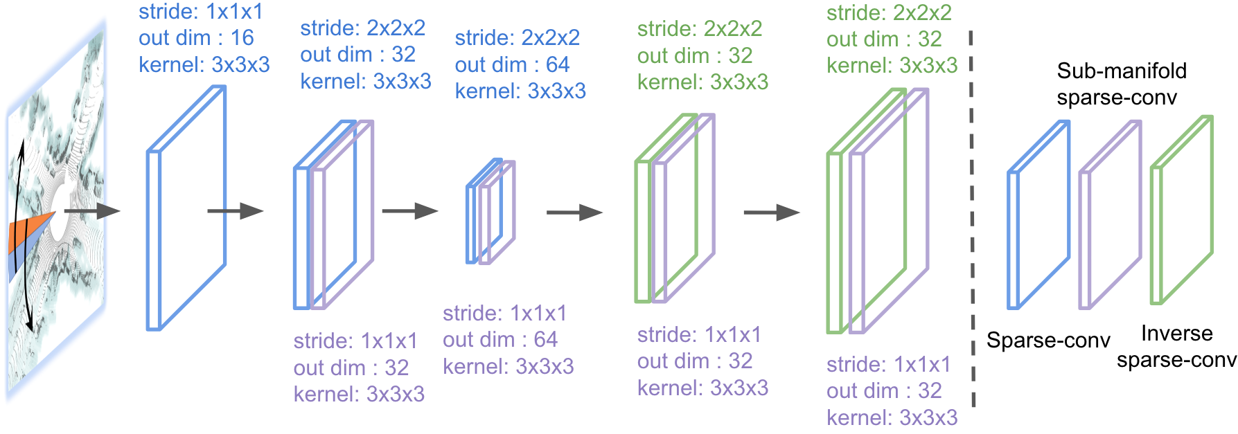
Figure 5: The network architecture of the shape occupancy network. The blue layers are regular sparse 3D convolutions (Graham 2015), the purple layers are sub-manifold sparse 3D convolutions (Graham and van der Maaten 2017), while the green layers are inverse sparse 3D convolutions (spatial up-sampling).

D.2 Detection Backbone Network $\Psi$

The backbone of the detection feature extraction network follows (Shi et al. 2020; Deng et al. 2020) but has thinner network layers. The point cloud is voxelized into Cartesian voxels where the features of each occupied voxel are the mean of the points’ xyz and features (e.g., intensity). Besides, the sparse probability tensor of object occupancy in the spherical coordinate has been transformed to the Cartesian coordinate $\mathcal{P}(\mathcal{O_{S}})$_⟂, so that two channels from $\mathcal{P}(\mathcal{O_{S}})$_⟂ can be concatenated with layers of $\Psi$. One channel holds the occupancy probability $\mathcal{P}(\mathcal{O_{S}})$ and the other holds the binary code if $\mathcal{P}(\mathcal{O_{S}})$ exists in a voxel. As visualized in Figure 6, three down-sampling layers down-sample the features to 8$\times$ smaller, which are fed into the region proposal network. The feature maps of the second, the third, and the final layer are further integrated with $\mathcal{P}(\mathcal{O_{S}})$_⟂ to form a local geometric feature $f_{geo}$, which supports the proposal refinement.

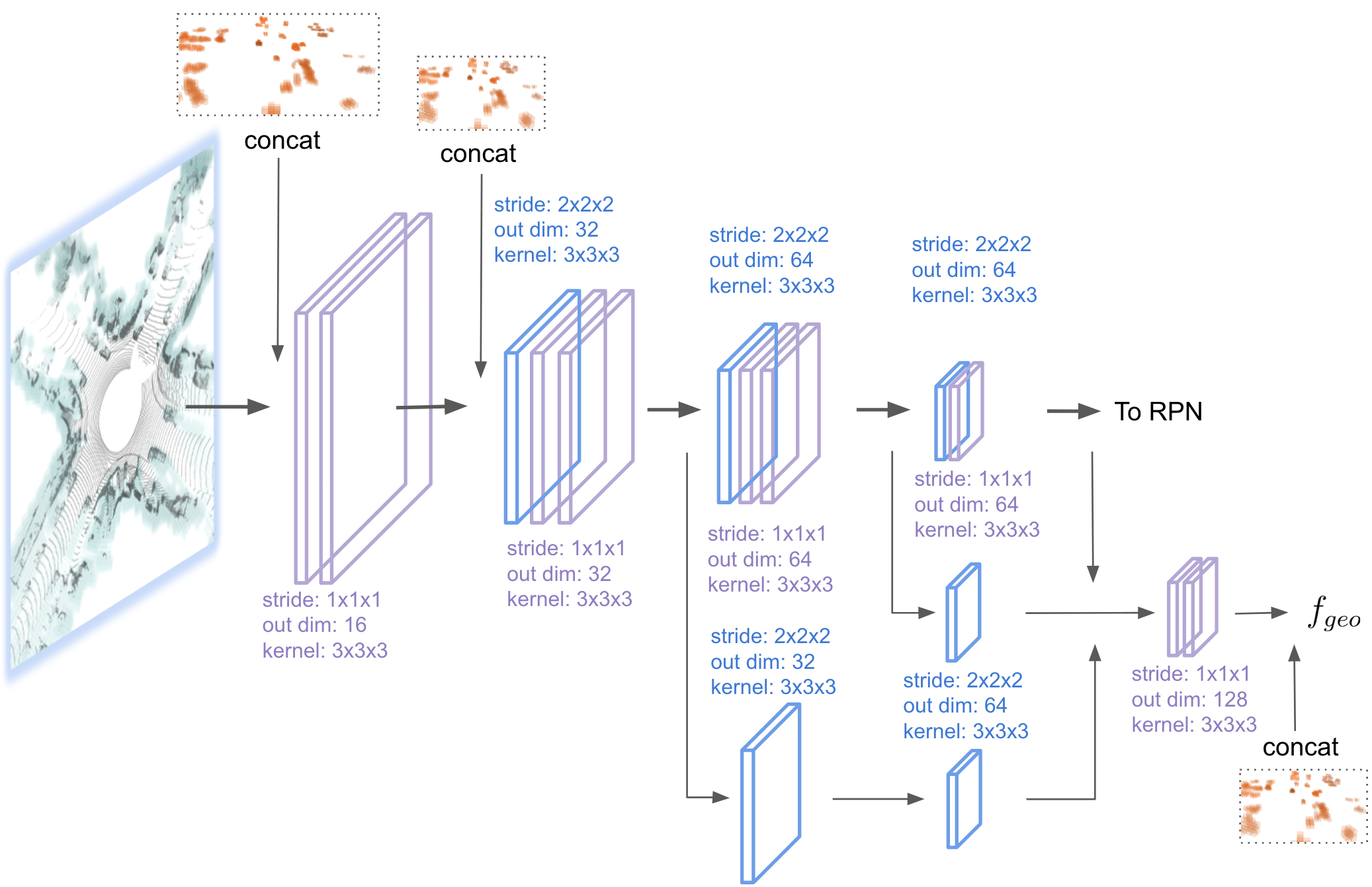
Figure 6: The architecture of the detection feature backbone network. The blue layers are the regular sparse 3D convolutions (Graham 2015) and the purple layers are sub-manifold sparse 3D convolutions (Graham and van der Maaten 2017).

D.3 Region Proposal Network

We stack the input features to bird-eye view 2D features. Then, a thinner version of the 2D convolution networks in (Lang et al. 2019; Yan et al. 2018) propagates the features and output residues of 2 anchors per class per grid on the output feature maps. Instead of dimensions of 256 as in (Shi et al. 2020; Deng et al. 2020), the intermediate feature maps in our 2D convolution networks has feature dimension of 128.

D.4 Proposal Refinement Network

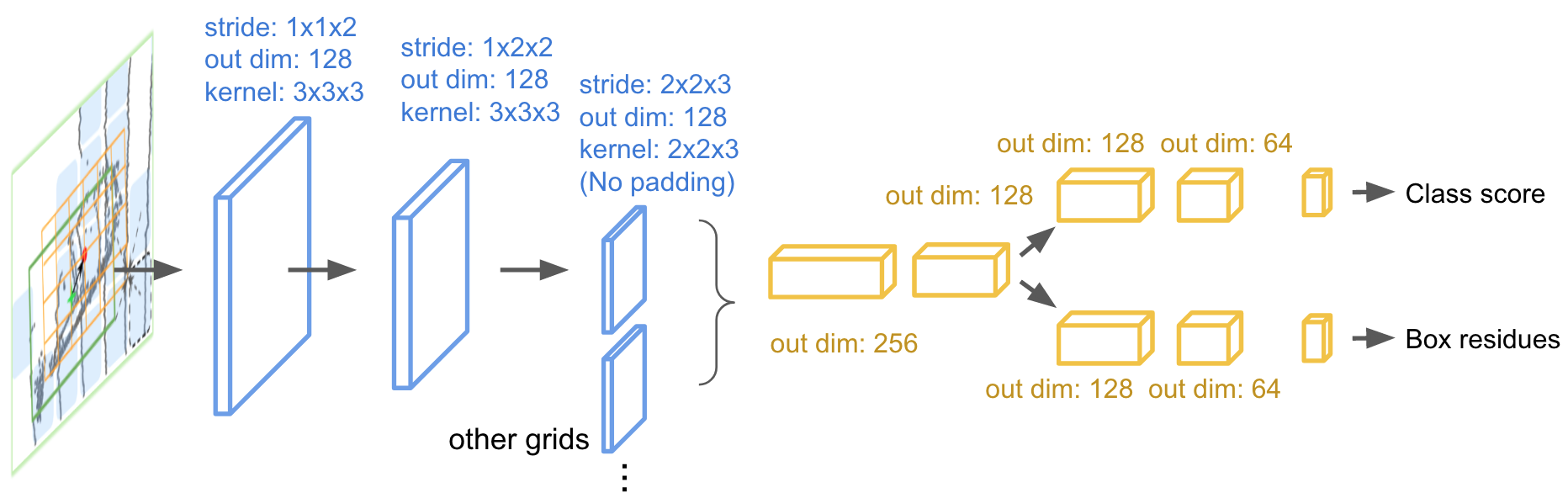
Figure 7: The architecture of the proposal refinement network in BtcDet’s detection pipeline. The blue layers are the regular sparse 3D convolutions (Graham 2015) and the yellow layers are fully-connected layers. The stride numbers correspond to Z, Y, X axis. In addition of the above network, We also aggregate the nearby points of the proposal.

A local grid of a region proposal has a grid size of (2, 4, 12) along the locally orientated axis of Z, Y, X. As shown in Figure 7, the aggregation network of the pooled local geometric features consist of three layers with the strides of (1,1,2), (1,2,2), (2,2,3). The first two layers have zero paddings, while the last layer does not. After that, we send them to several fully connected layers.

We have $3\times 3\times 3$ this kind of local grids for each proposal box. The center of a local grid ($x_{grid},y_{grid},z_{grid}$) have a shift away from the proposal center ($x_{p},y_{p},z_{p}$) by distances ($\Delta_{x}\in\{\pm\lambda,0\}\times w_{p},\Delta_{y}=\{\pm\lambda,0\}\times l_{p},\Delta_{z}=\{\pm\lambda,0\}\times h_{p}$), where $w_{p},l_{p},h_{p}$ is the width, length and height of the proposal box. We find $\lambda=0.25$ achieves the best results. The proposal refinement network aggregates results from all these shifted local grids and outputs the residues regression and the class confidence score, which lead to the final bounding box predictions.

Appendix E Occupancy Estimation of Complete Object Shapes

We show the evaluation of the occupancy estimation in Table 6. The results are averaged among all voxels in the regions of $\mathcal{R_{OC}}\cup\mathcal{R_{SM}}$. A prediction is considered positive if $\mathcal{P}(\mathcal{O_{S}})$ $>$ threshold. The metrics we evaluate are precision, recall, F1 score, accuracy, and object coverage. The object coverage is the percentage of all bounding boxes that contain at least one positive voxel ($\mathcal{P}(\mathcal{O_{S}})$ $>$ threshold). We show the measures on three thresholds of $0.3,0.5$, and $0.7$. The accuracy results under all thresholds are very high (¿99%) since the classes are extremely imbalanced. However, no matter under which threshold, we can achieve relatively high object coverage, which means the estimation is faithful enough for RPN and other downstream networks to rely on.

Threshold	Precision	Recall	F1 Score	Accuracy	Object Coverage
0.3	39.8 %	94.2 %	55.1 %	99.6 %	95.6 %
0.5	60.0 %	81.9 %	68.3 %	99.7 %	94.0 %
0.7	80.9 %	47.0 %	58.6 %	99.8 %	84.0 %

Table 6: The results of occupancy estimation. The model is trained on the KITTI’s train split and then evaluated on the KITTI’s val split. The precision, recall, F1 score, accuracy and object coverage are evaluated by setting $\mathcal{P}(\mathcal{O_{S}})$ $>$ the corresponding thresholds. Those metrics are evaluated considering all voxels in $\mathcal{R_{OC}}\cup\mathcal{R_{SM}}$. The object coverage is the the percentage of all bounding boxes that contain at least one voxel that is predicted as positive.

Appendix F More Comparison Results on the KITTI Test Set

We show more results of comparisons between BtcDet and other state-of-the-art detectors in Table 7. Because the average point number in pedestrians is smaller than other objects, the shape estimation is sensitive to a few observed points. Therefore, if the point number distribution of pedestrians in the test split is different, our model may not be able to provide an accurate shape occupancy estimation. As a result, BtcDet’s pedestrian detection on KITTI’s test split does not perform as well as on KITTI’s val split. We consider improving the results with this situation in our future works.

Method	Ped. 3D $AP_{R40}$				Car 3D $AP_{R40}$				Cyc. 3D $AP_{R40}$
	Easy	Mod.	Hard	mAP	Easy	Mod.	Hard	mAP	Easy	Mod.	Hard	mAP
F-PointNet (Qi et al. 2018)	50.53	42.15	38.08	43.59	82.19	69.79	60.59	70.86	72.27	56.12	49.01	59.13
AVOD-FPN (Ku et al. 2018)	50.46	42.27	39.04	43.92	83.07	71.76	65.73	73.52	63.76	50.55	44.93	53.08
F-ConvNet (Wang and Jia 2019)	52.16	43.38	38.8	44.78	87.36	76.39	66.69	76.81	81.98	65.07	56.54	67.86
Uber-MMF (Liang et al. 2019)	-	-	-	-	88.40	77.43	70.22	78.68	-	-	-	-
EPNet (Huang et al. 2020)	52.79	44.38	41.29	46.15	89.81	79.28	74.59	81.23	-	-	-	-
CLOCsPVCas (Pang et al. 2020)	-	-	-	-	88.94	80.67	77.15	82.25	-	-	-	-
3D-CVF (Yoo et al. 2020)	-	-	-	-	89.20	80.05	73.11	80.79	-	-	-	-
SECOND (Yan et al. 2018)	48.73	40.57	37.77	42.36	83.34	72.55	65.82	73.90	71.33	52.08	45.83	56.41
PointPillars (Lang et al. 2019)	51.45	41.92	38.89	44.09	82.58	74.31	68.99	75.29	77.10	58.65	51.92	62.56
PointRCNN (Shi et al. 2019a)	47.98	39.37	36.01	41.12	86.96	76.50	71.39	78.28	74.96	58.82	52.53	62.10
3D Iou Loss (Zhou et al. 2019)	-	-	-	-	86.16	75.64	70.70	77.50	-	-	-	-
Fast PointRCNN (Chen et al. 2019)	-	-	-	-	85.29	77.40	70.24	77.64	-	-	-	-
STD (Yang et al. 2019)	53.29	42.47	38.35	44.70	87.95	79.71	75.09	80.92	78.69	61.59	55.30	65.19
SegVoxelNet (Yi et al. 2020)	-	-	-	-	86.04	76.13	70.76	77.64	-	-	-	-
VoxelFPN (Kuang et al. 2020)	-	-	-	-	85.63	76.70	69.44	77.26	-	-	-	-
HotSpotNet (Chen et al. 2020)	53.10	45.37	41.47	46.65	87.60	78.31	73.34	79.75	82.59	65.95	59.00	69.18
PartA2 (Shi et al. 2020)	53.10	43.35	40.06	45.50	87.81	78.49	73.51	79.94	79.17	63.52	56.93	66.54
SERCNN (Zhou et al. 2020a)	-	-	-	-	87.74	78.96	74.14	80.28	-	-	-	-
Point-GNN (Shi and Rajkumar 2020)	51.92	43.77	40.14	45.28	88.33	79.47	72.29	80.03	78.60	63.48	57.08	66.39
3DSSD (Yang et al. 2020)	50.64	43.09	39.65	44.46	88.36	79.57	74.55	80.83	82.48	64.10	56.90	67.83
SA-SSD (He et al. 2020)	-	-	-	-	88.75	79.79	74.16	80.90	-	-	-	-
Asso-3Ddet (Du et al. 2020)	-	-	-	-	85.99	77.40	70.53	77.97	-	-	-	-
PV-RCNN (Shi et al. 2020)	52.17	43.29	40.29	45.25	90.25	81.43	76.82	82.83	78.60	63.71	57.65	66.65
Voxel R-CNN (Deng et al. 2020)	-	-	-	-	90.90	81.62	77.06	83.19	-	-	-	-
CIA-SSD (Zheng et al. 2021)	-	-	-	-	89.59	80.28	72.87	80.91	-	-	-	-
TANet (Liu et al. 2020)	53.72	44.34	40.49	46.18	83.81	75.38	67.66	75.62	73.84	59.86	53.46	62.39
BtcDet (Ours)	47.80	41.63	39.30	42.91	90.64	82.86	78.09	83.86	82.81	68.68	61.81	71.10

Table 7: Comparison results for all three classes of objects on the KITTI test set, evaluated by the 3D Average Precision (AP) of 40 recall thresholds (R40) on the KITTI server. The mAPs are averaged over the APs of easy, moderate, and hard objects.

Appendix G More Visualization for the Complete Object Shape Approximation

We show more results of the assembled complete object shapes of cyclists and pedestrians in this section. Figure 8 visualizes the process for cyclists which includes mirroring both source and target objects. Figure 9 and 10 visualizes the process for pedestrians which does not mirror the objects since pedestrians are less likely to be symmetric. The blue points are the points of the target object and the red points are the points of the source objects. The assembled object faithfully covers the originally partially observed parts of the target objects and provides reasonable recovery points in the shape miss regions of the target objects.

Figure 8: The assembly process to approximate the complete object shapes for cyclists on KITTI (Geiger et al. 2013). The red points are from the source objects, the blue points are from target objects, the complete shape of the target objects are approximated by borrowing the points from the selected source objects.

Figure 9: The assembly process to approximate the complete shapes for pedestrians on KITTI (Geiger et al. 2013). The red points are from the source objects, the blue points are from target objects, the complete shape of the target objects are approximated by borrowing the points from the selected source objects (red).

Figure 10: The assembly process to approximate the complete shapes for pedestrians on KITTI (Geiger et al. 2013). The red points are from the source objects, the blue points are from target objects, the complete shape of the target objects are approximated by borrowing the points from the selected source objects (red).

Appendix H Visualization of the Occupancy Probability $\mathcal{P}(\mathcal{O_{S}})$

We show the qualitative results of the occupancy probability for vehicle objects on the Waymo Open Dataset (Sun et al. 2019). Figure 11 contains zoomed in views of the occupancy probability while Figure 12 contains full scene views. The higher probability one is estimated, the larger opacity we apply to the spherical voxel.

Figure 11: The zoomed in views of the predicted occupancy probability for vehicle objects on the Waymo Open Dataset (Sun et al. 2019). The higher probability it is predicted, the larger opacity we apply to the spherical voxel.

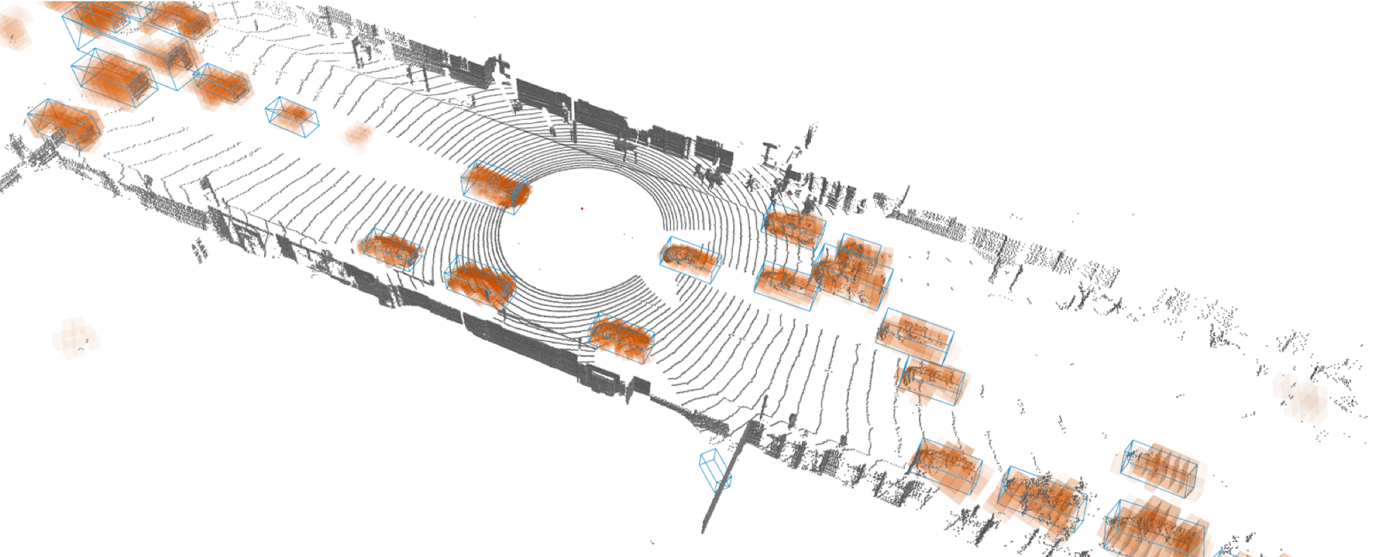
Figure 12: The full scene views of the predicted occupancy probability for vehicle objects on the Waymo Open Dataset (Sun et al. 2019). The higher probability it is predicted, the larger opacity we apply to the spherical voxel.

References

- Chen et al. (2020) Chen, Q.; Sun, L.; Wang, Z.; Jia, K.; and Yuille, A. 2020. Object as hotspots: An anchor-free 3d object detection approach via firing of hotspots. In European Conference on Computer Vision, 68–84. Springer.
- Chen et al. (2017) Chen, X.; Ma, H.; Wan, J.; Li, B.; and Xia, T. 2017. Multi-view 3D Object Detection Network for Autonomous Driving. 2017 IEEE Conference on Computer Vision and Pattern Recognition (CVPR), 6526–6534.
- Chen et al. (2019) Chen, Y.; Liu, S.; Shen, X.; and Jia, J. 2019. Fast point r-cnn. In Proceedings of the IEEE International Conference on Computer Vision, 9775–9784.
- Deng et al. (2020) Deng, J.; Shi, S.; Li, P.; Zhou, W.; Zhang, Y.; and Li, H. 2020. Voxel R-CNN: Towards High Performance Voxel-based 3D Object Detection. arXiv:2012.15712.
- Du et al. (2020) Du, L.; Ye, X.; Tan, X.; Feng, J.; Xu, Z.; Ding, E.; and Wen, S. 2020. Associate-3Ddet: Perceptual-to-Conceptual Association for 3D Point Cloud Object Detection. In Proceedings of the IEEE/CVF Conference on Computer Vision and Pattern Recognition, 13329–13338.
- Follmann et al. (2019) Follmann, P.; König, R.; Härtinger, P.; Klostermann, M.; and Böttger, T. 2019. Learning to see the invisible: End-to-end trainable amodal instance segmentation. In 2019 IEEE Winter Conference on Applications of Computer Vision (WACV), 1328–1336. IEEE.
- Ge et al. (2020) Ge, R.; Ding, Z.; Hu, Y.; Wang, Y.; Chen, S.; Huang, L.; and Li, Y. 2020. Afdet: Anchor free one stage 3d object detection. arXiv preprint arXiv:2006.12671.
- Geiger et al. (2013) Geiger, A.; Lenz, P.; Stiller, C.; and Urtasun, R. 2013. Vision meets robotics: The kitti dataset. The International Journal of Robotics Research, 32(11): 1231–1237.
- Graham (2015) Graham, B. 2015. Sparse 3D convolutional neural networks. arXiv preprint arXiv:1505.02890.
- Graham and van der Maaten (2017) Graham, B.; and van der Maaten, L. 2017. Submanifold sparse convolutional networks. arXiv preprint arXiv:1706.01307.
- He et al. (2020) He, C.; Zeng, H.; Huang, J.; Hua, X.-S.; and Zhang, L. 2020. Structure Aware Single-stage 3D Object Detection from Point Cloud. In Proceedings of the IEEE Conference on Computer Vision and Pattern Recognition.
- Hu et al. (2020) Hu, P.; Ziglar, J.; Held, D.; and Ramanan, D. 2020. What You See is What You Get: Exploiting Visibility for 3D Object Detection. In Proceedings of the IEEE/CVF Conference on Computer Vision and Pattern Recognition (CVPR).
- Huang et al. (2020) Huang, T.; Liu, Z.; Chen, X.; and Bai, X. 2020. Epnet: Enhancing point features with image semantics for 3d object detection. In European Conference on Computer Vision, 35–52. Springer.
- Jiang et al. (2018) Jiang, B.; Luo, R.; Mao, J.; Xiao, T.; and Jiang, Y. 2018. Acquisition of localization confidence for accurate object detection. In Proceedings of the European Conference on Computer Vision (ECCV), 784–799.
- Kingma and Ba (2014) Kingma, D. P.; and Ba, J. 2014. Adam: A method for stochastic optimization. arXiv preprint arXiv:1412.6980.
- Ku et al. (2018) Ku, J.; Mozifian, M.; Lee, J.; Harakeh, A.; and Waslander, S. L. 2018. Joint 3d proposal generation and object detection from view aggregation. In 2018 IEEE/RSJ International Conference on Intelligent Robots and Systems (IROS), 1–8. IEEE.
- Kuang et al. (2020) Kuang, H.; Wang, B.; An, J.; Zhang, M.; and Zhang, Z. 2020. Voxel-FPN: Multi-scale voxel feature aggregation for 3D object detection from LIDAR point clouds. Sensors, 20(3): 704.
- Lang et al. (2019) Lang, A. H.; Vora, S.; Caesar, H.; Zhou, L.; Yang, J.; and Beijbom, O. 2019. Pointpillars: Fast encoders for object detection from point clouds. In Proceedings of the IEEE Conference on Computer Vision and Pattern Recognition, 12697–12705.
- Li et al. (2019) Li, B.; Ouyang, W.; Sheng, L.; Zeng, X.; and Wang, X. 2019. Gs3d: An efficient 3d object detection framework for autonomous driving. In Proceedings of the IEEE Conference on Computer Vision and Pattern Recognition, 1019–1028.
- Li et al. (2021) Li, Z.; Yao, Y.; Quan, Z.; Yang, W.; and Xie, J. 2021. SIENet: Spatial Information Enhancement Network for 3D Object Detection from Point Cloud. arXiv preprint arXiv:2103.15396.
- Liang et al. (2019) Liang, M.; Yang, B.; Chen, Y.; Hu, R.; and Urtasun, R. 2019. Multi-task multi-sensor fusion for 3d object detection. In Proceedings of the IEEE Conference on Computer Vision and Pattern Recognition, 7345–7353.
- Lin et al. (2017) Lin, T.-Y.; Goyal, P.; Girshick, R.; He, K.; and Dollár, P. 2017. Focal loss for dense object detection. In Proceedings of the IEEE international conference on computer vision, 2980–2988.
- Liu et al. (2018) Liu, Y.; Jing, X.-Y.; Nie, J.; Gao, H.; Liu, J.; and Jiang, G.-P. 2018. Context-aware three-dimensional mean-shift with occlusion handling for robust object tracking in RGB-D videos. IEEE Transactions on Multimedia, 21(3): 664–677.
- Liu et al. (2020) Liu, Z.; Zhao, X.; Huang, T.; Hu, R.; Zhou, Y.; and Bai, X. 2020. Tanet: Robust 3d object detection from point clouds with triple attention. In Proceedings of the AAAI Conference on Artificial Intelligence, volume 34, 11677–11684.
- Najibi et al. (2020) Najibi, M.; Lai, G.; Kundu, A.; Lu, Z.; Rathod, V.; Funkhouser, T.; Pantofaru, C.; Ross, D.; Davis, L. S.; and Fathi, A. 2020. Dops: Learning to detect 3d objects and predict their 3d shapes. In Proceedings of the IEEE/CVF conference on computer vision and pattern recognition, 11913–11922.
- Pan et al. (2021) Pan, Y.; Xiao, P.; He, Y.; Shao, Z.; and Li, Z. 2021. MULLS: Versatile LiDAR SLAM via Multi-metric Linear Least Square. arXiv preprint arXiv:2102.03771.
- Pang et al. (2020) Pang, S.; Morris, D.; and Radha, H. 2020. CLOCs: Camera-LiDAR Object Candidates Fusion for 3D Object Detection. arXiv preprint arXiv:2009.00784.
- Qi et al. (2019a) Qi, C. R.; Litany, O.; He, K.; and Guibas, L. J. 2019a. Deep hough voting for 3d object detection in point clouds. In Proceedings of the IEEE/CVF International Conference on Computer Vision, 9277–9286.
- Qi et al. (2018) Qi, C. R.; Liu, W.; Wu, C.; Su, H.; and Guibas, L. J. 2018. Frustum pointnets for 3d object detection from rgb-d data. In Proceedings of the IEEE conference on computer vision and pattern recognition, 918–927.
- Qi et al. (2019b) Qi, L.; Jiang, L.; Liu, S.; Shen, X.; and Jia, J. 2019b. Amodal instance segmentation with kins dataset. In Proceedings of the IEEE/CVF Conference on Computer Vision and Pattern Recognition, 3014–3023.
- Reddy et al. (2019) Reddy, N. D.; Vo, M.; and Narasimhan, S. G. 2019. Occlusion-net: 2d/3d occluded keypoint localization using graph networks. In Proceedings of the IEEE/CVF Conference on Computer Vision and Pattern Recognition, 7326–7335.
- Saleh et al. (2021) Saleh, K.; Szénási, S.; and Vámossy, Z. 2021. Occlusion Handling in Generic Object Detection: A Review. In 2021 IEEE 19th World Symposium on Applied Machine Intelligence and Informatics (SAMI), 000477–000484. IEEE.
- Shi et al. (2020) Shi, S.; Guo, C.; Jiang, L.; Wang, Z.; Shi, J.; Wang, X.; and Li, H. 2020. Pv-rcnn: Point-voxel feature set abstraction for 3d object detection. In Proceedings of the IEEE/CVF Conference on Computer Vision and Pattern Recognition, 10529–10538.
- Shi et al. (2019a) Shi, S.; Wang, X.; and Li, H. 2019a. Pointrcnn: 3d object proposal generation and detection from point cloud. In Proceedings of the IEEE Conference on Computer Vision and Pattern Recognition, 770–779.
- Shi et al. (2019b) Shi, S.; Wang, Z.; Shi, J.; Wang, X.; and Li, H. 2019b. From Points to Parts: 3D Object Detection from Point Cloud with Part-aware and Part-aggregation Network. arXiv preprint arXiv:1907.03670.
- Shi et al. (2020) Shi, S.; Wang, Z.; Shi, J.; Wang, X.; and Li, H. 2020. From Points to Parts: 3D Object Detection from Point Cloud with Part-aware and Part-aggregation Network. IEEE Transactions on Pattern Analysis and Machine Intelligence, 1–1.
- Shi and Rajkumar (2020) Shi, W.; and Rajkumar, R. 2020. Point-gnn: Graph neural network for 3d object detection in a point cloud. In Proceedings of the IEEE/CVF Conference on Computer Vision and Pattern Recognition, 1711–1719.
- Sun et al. (2019) Sun, P.; Kretzschmar, H.; Dotiwalla, X.; Chouard, A.; Patnaik, V.; Tsui, P.; Guo, J.; Zhou, Y.; Chai, Y.; Caine, B.; Vasudevan, V.; Han, W.; Ngiam, J.; Zhao, H.; Timofeev, A.; Ettinger, S.; Krivokon, M.; Gao, A.; Joshi, A.; Zhang, Y.; Shlens, J.; Chen, Z.; and Anguelov, D. 2019. Scalability in Perception for Autonomous Driving: Waymo Open Dataset. arXiv:1912.04838.
- Wang et al. (2020) Wang, Y.; Fathi, A.; Kundu, A.; Ross, D.; Pantofaru, C.; Funkhouser, T.; and Solomon, J. 2020. Pillar-based object detection for autonomous driving. arXiv preprint arXiv:2007.10323.
- Wang and Jia (2019) Wang, Z.; and Jia, K. 2019. Frustum ConvNet: Sliding Frustums to Aggregate Local Point-Wise Features for Amodal 3D Object Detection. In 2019 IEEE/RSJ International Conference on Intelligent Robots and Systems (IROS), 1742–1749. IEEE.
- Xu et al. (2020) Xu, Q.; Sun, X.; Wu, C.-Y.; Wang, P.; and Neumann, U. 2020. Grid-gcn for fast and scalable point cloud learning. In Proceedings of the IEEE/CVF Conference on Computer Vision and Pattern Recognition, 5661–5670.
- Xu et al. (2021) Xu, Q.; Zhou, Y.; Wang, W.; Qi, C. R.; and Anguelov, D. 2021. Spg: Unsupervised domain adaptation for 3d object detection via semantic point generation. In Proceedings of the IEEE/CVF International Conference on Computer Vision, 15446–15456.
- Yan et al. (2020) Yan, X.; Gao, J.; Li, J.; Zhang, R.; Li, Z.; Huang, R.; and Cui, S. 2020. Sparse single sweep lidar point cloud segmentation via learning contextual shape priors from scene completion. arXiv preprint arXiv:2012.03762.
- Yan et al. (2018) Yan, Y.; Mao, Y.; and Li, B. 2018. Second: Sparsely embedded convolutional detection. Sensors, 18(10): 3337.
- Yang et al. (2020) Yang, Z.; Sun, Y.; Liu, S.; and Jia, J. 2020. 3dssd: Point-based 3d single stage object detector. In Proceedings of the IEEE/CVF Conference on Computer Vision and Pattern Recognition, 11040–11048.
- Yang et al. (2019) Yang, Z.; Sun, Y.; Liu, S.; Shen, X.; and Jia, J. 2019. Std: Sparse-to-dense 3d object detector for point cloud. In Proceedings of the IEEE International Conference on Computer Vision, 1951–1960.
- Ye et al. (2020) Ye, M.; Xu, S.; and Cao, T. 2020. Hvnet: Hybrid voxel network for lidar based 3d object detection. In Proceedings of the IEEE/CVF conference on computer vision and pattern recognition, 1631–1640.
- Yi et al. (2020) Yi, H.; Shi, S.; Ding, M.; Sun, J.; Xu, K.; Zhou, H.; Wang, Z.; Li, S.; and Wang, G. 2020. Segvoxelnet: Exploring semantic context and depth-aware features for 3d vehicle detection from point cloud. In 2020 IEEE International Conference on Robotics and Automation (ICRA), 2274–2280. IEEE.
- Yoo et al. (2020) Yoo, J. H.; Kim, Y.; Kim, J. S.; and Choi, J. W. 2020. 3d-cvf: Generating joint camera and lidar features using cross-view spatial feature fusion for 3d object detection. arXiv preprint arXiv:2004.12636, 3.
- Zhang et al. (2018) Zhang, S.; Wen, L.; Bian, X.; Lei, Z.; and Li, S. Z. 2018. Occlusion-aware R-CNN: detecting pedestrians in a crowd. In Proceedings of the European Conference on Computer Vision (ECCV), 637–653.
- Zheng et al. (2021) Zheng, W.; Tang, W.; Chen, S.; Jiang, L.; and Fu, C.-W. 2021. CIA-SSD: Confident IoU-Aware Single-Stage Object Detector From Point Cloud. In AAAI.
- Zhou et al. (2019) Zhou, D.; Fang, J.; Song, X.; Guan, C.; Yin, J.; Dai, Y.; and Yang, R. 2019. Iou loss for 2d/3d object detection. In 2019 International Conference on 3D Vision (3DV), 85–94. IEEE.
- Zhou et al. (2020a) Zhou, D.; Fang, J.; Song, X.; Liu, L.; Yin, J.; Dai, Y.; Li, H.; and Yang, R. 2020a. Joint 3D Instance Segmentation and Object Detection for Autonomous Driving. In Proceedings of the IEEE/CVF Conference on Computer Vision and Pattern Recognition (CVPR).
- Zhou et al. (2020b) Zhou, Y.; Sun, P.; Zhang, Y.; Anguelov, D.; Gao, J.; Ouyang, T.; Guo, J.; Ngiam, J.; and Vasudevan, V. 2020b. End-to-end multi-view fusion for 3d object detection in lidar point clouds. In Conference on Robot Learning, 923–932.
- Zhou and Tuzel (2018) Zhou, Y.; and Tuzel, O. 2018. Voxelnet: End-to-end learning for point cloud based 3d object detection. In Proceedings of the IEEE Conference on Computer Vision and Pattern Recognition, 4490–4499.