Causal-based Time Series Domain Generalization for Vehicle Intention Prediction

Abstract

The purpose of this document is to provide both the basic paper template and submission guidelines. Abstracts should be a single paragraph, between 4–6 sentences long, ideally. Gross violations will trigger corrections at the camera-ready phase.

Keywords: CoRL, Robots, Learning

1 Introduction

1.1 Random

1.1.1 Work Summary

• (We formulate vehicle intention prediction problem using structural causal model and recurrent latent variable model. We demonstrate that our proposed problem formulation is able to generalize well on out-of-distribution testing data, which is important in order for autonomous vehicle to navigate under unseen urban environments.)

• In this paper, we propose to learn a common representation of time-series data that can be transferred across domains. Specifically, we first use variational methods to produce a latent representation that captures underlying temporal latent dependencies in the data. We then utilize a structural causal model to identify a correct invariant condition needed for our domain generalization task and extract corresponding causal (domain-independent) features from the previously learned latent representation.

• Many of the current domain generalization approaches work very well for non-sequential data but are not suitable for multivariate time-series data as they do not usually capture the temporal dependencies present in the data [xx]. For sequential data, methods such as dynamic Bayesian Network (DBN)[xx] and Recurrent Neural Networks (RNN)[xx] have been utilized to learn latent feature representations that are domain invariant. However, these works are either limited to model simple state transition structure or incapable of capturing complex latent dependencies of time-series data. Therefore, in this work, we draw inspiration from the Variational Recurrent Neural Network [xx] and use variational methods to learn a latent representation that captures underlying temporal latent dependencies. These representations will then be used for domain generalization task.

• As discussed earlier, for highly structured sequential data such as interactive trajectories, it is important to capture complex latent dependencies which are needed to perform domain generalization of time-series data.

• Moreover, we assume that each input data is constructed from a mix of inherent (causal) and domain-dependent (non-causal) features. Consequently, the captured temporal latent dependencies from sequential data also contain both causal and non-causal features. Therefore, we construct a structural causal model inspired from data generation process and propose to learn an invariant representation from temporal latent dependencies of input data for domain generalization, where the learning scheme is based on an invariant condition identified from the causal model.

1.1.2 Advantages of our approach

• (State why we need to extract temporal latent dependencies from data.)…..

• (State why we utilize structural causal model.)

1.2 Contribution

1. To the best of our knowledge, this is the first model trying to tackle time series domain generalization problem for vehicle intention prediction task.

2. Specifically, based on a structural causal model, we proposed to learn an invariant representation for time series vehicle interaction data and utilize the learned representation for domain generalization.

1.3 Motivation

Figure 1 illustrates the motivation of this work. Consider two vehicles interact with each other under two different scenarios. For better understanding of the concept, we temporarily make the following assumptions for both interaction cases:

• Same relative road priority of two roads that two vehicles are driving on.

• Same drivers driving the two cars, whose driving styles are consistence across different scenarios [xx].

• Same distance towards two roads’ conflict/intersect point (i.e. black dot) for both vehicles when interaction begins.

There are also two main differences between two cases: (1) Different topological road structure of two intersected roads, which can be regarded as different domains; (2) Two drivers have different driving styles and the driver in the red car is more aggressive than the driver in the blue car, which information is actually unavailable when making predictions.

Based on previous assumptions and settings, for a given interaction period, a plausible velocity profile of two vehicles is shown in the second row of Fig. 1 for both cases. The goal is to predict the intention of any selected vehicle, which can be the intent of passing or yielding the other car. According to the plots, whether the red car yields or passes the blue car doesn’t relate much to the domain information but depends more on two drivers’ personal information (e.g. driving style) and their initial states. Specifically, the geometry of the roads could affect several factors such as when two vehicles start noticing each other, when the road negotiation begins, and when drivers agree on who will go first. All these factors could then influence the velocity profiles of two vehicles but won’t have much effects on the intention of two vehicles when the aforementioned assumptions hold. In other words, if two vehicles encounter each other twice under different domains, as long as the three assumptions are true, the aggressive driver will always prefer passing than yielding the less aggressive driver.

Therefore, it is the features that relate to two drivers’ information and their internal relations (e.g. highlighted in cyan), instead of those that relate to domain itself (e.g. highlighted in orange), determine the intention. Hence, we construct a model for the data collection process that assumes each input data (i.e. vehicle trajectories) is constructed from a mix of causal and non-causal features. We consider domain as a main intervention that changes the non-causal features of an input data, and propose that an ideal intention predictor should depends only on the causal features.

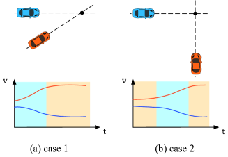
Figure 1: Illustration of the problem motivation.

2 Related Works

3 Method

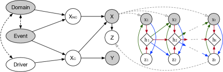
Figure 2: Illustration of the overall framework. Observed quantities are shown as shaded nodes; nodes of latent quantities are transparent. A directed black edge ($\relbar\joinrel\mathrel{\RHD}$) denotes a causal relationship; dashed bidirectional edges ($\LHD\makebox[6.99997pt]{\xdotfill{.4pt}}\RHD$) denote correlation; hollow dashed arrows ($\makebox[6.99997pt]{\xdotfill{.4pt}}\rhd$) denote an inclusion relationship. Blue lines ($\color[rgb]{0,0,1}\relbar\joinrel\mathrel{\RHD}$) denote the inference process, $q(z_{t}|x_{\leq t},z_{<t})$; green lines ($\color[rgb]{0,0.5,0}\relbar\joinrel\mathrel{\RHD}$) represent the generation process, $p(x_{t}|z_{\leq t,x_{<t}})$; red lines ($\color[rgb]{0.75,0,0}\relbar\joinrel\mathrel{\RHD}$) show the recurrence process where $h_{t}$ is informed by $h_{t-1}$, which is informed by $z_{t-1}$ and $x_{t-1}$.

In this section, we present a domain generalization method for vehicle intention prediction based on time-series data. Specifically, we name our model as Causal-based Time Series Domain Generalization (CTSDG), which captures and transfers inter-vehicle causal relations as well as temporal latent dependencies across domains via domain-invariant representations.

3.1 Problem Formulation and Overview

Consider a classification task where the learning algorithm has access to i.i.d. data from $m$ domains, $\{(d_{i},\mathbf{x}_{i},\mathbf{y}_{i})\}_{i=1}^{n}\sim(D_{m},\mathcal{X},\mathcal{Y})^{n}$ where $d^{i}\in D_{m}$, $D_{m}\subset\mathcal{D}$ as a set of $m$ domains, and $\mathbf{x}_{i}=(x_{t}^{i})_{t=1}^{T}$ denotes a multivariate time series with $x_{t}^{i}\in\mathbb{R}^{H}$. In this work, given historical trajectories of interacting vehicle pairs, the domain generalization task is to learn a single classifier (i.e. predict pass or yield intention) that generalizes well to unseen domains $d^{\prime}\notin D_{m}$ and to new data from the same domains [xx].

3.2 A Causal View of Interactive Data Generating Process

3.2.1 Structural Causal Model (SCM)

Figure 2 shows a SCM that describes how interactive trajectories are generated by two drivers after encountering each other. The detailed meaning of each node variable in our task is listed below:

• Domain ($D$): Each driving scenario can be regarded as a different domain, which contains information/properties such as road topology, speed limit, and traffic rules. (maybe need to assume that all domains should belongs to a same distribution (i.e. merging scene instead of highway))

• Event ($E$): Observable variables relate to the interaction event such as initial states of both vehicles and the length of interaction.

• Driver ($O$): Unobservable variables relate each driver’s personal information such as the aggressiveness level and whether he/she obeys traffic rules.

• Causal features ($X_{C}$): High-level causal features related to driver information, which are used by humans to label the intention (these causal features are related to temporal information).

• Non-causal features ($X_{A}$): Domain dependent features produced by combination of the domain and the event.(these causal features are related to temporal information).

• Input Data ($X$): Vehicle interactive trajectories, which can be regarded as sequential multivariate data.

• Latent variables ($Z$): Latent representations extracted from time-series data.

• Labels ($Y$): Vehicle intention labels. For two vehicle interaction cases, we normally assign a binary label to represent selected driver’s intention of either passing or yielding the other car at a given time step.

Each pair of interactive trajectories is obtained by first selecting two vehicles in a scene (i.e. domain $D$) that have potential interaction with each other and the unobservable drivers’ information are stored in $O$. Then, a desired starting time and interaction period (i.e. variables related to $E$) are selected. The driving scenario corresponds to domain-depended high-level features $X_{A}$. Both $O$ and $E$ correspond to high-level causal features $X_{C}$ which are used by human to label the intention $Y$. Finally, $X_{C}$ and $X_{A}$ construct the interactive trajectories $X$.

We can write the following non-parametric equations corresponding to the SCM:

$$\mathbf{x}_{c} =g_{xc}(\mathbf{e,o}) \mathbf{x}_{a} =g_{xa}(d,\mathbf{o})$$

$$\mathbf{x} =g_{x}(\mathbf{x}_{c},\mathbf{x}_{a}) y =h(\mathbf{x}_{c}) \mathbf{z}=r(\mathbf{x})$$

where $g_{xc}$, $g_{xa}$, $g_{x}$, $h_{y}$, and $h_{z}$ are general non-parametric functions. Moreover, SCM contains conditional-independence conditions that all data distributions $\mathcal{P}$ must satisfy through the d-separation concept [xx].

3.2.2 Invariance Condition

According to Fig 2, $X_{C}$ is the node that causes $Y$ and by d-separation, the intention label is independent of domain conditioned on $X_{C}$, $Y\perp\!\!\!\!\perp D|X_{C}$. In other word, if such a $X_{C}$ can be found, then the distribution of Y conditional on $X_{C}$ is invariant under transferring from the source domains to the target domains…..

Therefore, our intention prediction task is to learn $y$ as $h(\mathbf{x}_{c})$ where $h:\mathcal{C}\rightarrow\mathcal{Y}$. However, since $X_{C}$ is unobserved, we need to learn $y$ through observed trajectories $X$. Specifically, we utilize a representation function $q:\mathcal{X}\rightarrow\mathcal{Z}$ to map the input space to a latent space and a hypothesis function $\phi:\mathcal{Z}\rightarrow\mathcal{C}$ to map the latent space to $X_{C}$. Together, $h(\phi(q(x)))$ leads to the desired intention predictor $f:\mathcal{X}\rightarrow\mathcal{Y}$ and the corresponding prediction loss can be written as:

$$\mathcal{L}_{y}=\mathcal{L}_{\alpha}(h(\phi(q(X))),Y),$$ (1)

where $\mathcal{L}_{\alpha}$ is the classification loss such as a binary or categorical cross-entropy.

In addition, by the d-separation, $X_{C}$ also need to satisfy an invariance condition: $X_{C}\perp\!\!\!\!\perp D|\{E,O\}$, which means $X_{C}$ does not change with different domains for if both event and driver remain the same. However, driver information is unobservable and in many dataset there many not be an exactly match based on a same event across domains. Alternatively, we assume that the distance over $X_{C}$ between same-class inputs from different domains is bounded by $\delta$, which provides an alternative invariance condition that is consistent with the conditional independencies of $X_{C}$. (Proof shown in appendix.) If a dataset has low $\delta$, then there is a high chance of learning a good representation that is close to $X_{C}$. Therefore, we would like to minimize the following objective along with the prediction loss:

$$\mathcal{L}_{r}=\sum_{\Omega(\mathbf{x}_{j},\mathbf{x}_{k})=1;d_{j}\neq d_{k}}\mathcal{L}_{\beta}(\phi(q(\mathbf{x}_{j}^{(d_{j})})),\phi(q(\mathbf{x}_{k}^{(d_{k})}))),$$ (2)

where $\mathcal{L}_{\beta}$ is the distance metric such as $\ell_{2}$, and $\Omega:\mathcal{X}\times\mathcal{X}\rightarrow\{0,1\}$ is a match function such that pairs having $\Omega(\mathbf{x}_{j},\mathbf{x}_{k})=1$ have low difference in their causal features.

3.3 Recurrent Latent Variable Model

As discussed earlier, simply use deep learning models like RNN cannot efficiently model complex dependencies …From our SCM, we observe that $Z\perp\!\!\!\!\perp D|X$. Talk about the relation with previously mentioned representation function q.

To explicitly model the dependencies between latent random variable across time steps, our proposed CTSDG model utilizes Variational Recurrent Neural Networks (VRNN) [xx]. The VRNN contains a VAE at every time step and these VAEs are conditioned on previous auto-encoders via the hidden state variable $h_{t-1}$ of an RNN. Therefore, for each time step of $x_{t}^{i}$, a latent random variable $z_{t}^{i}$ is learned following the equation:

$$z_{t}^{i}|x_{t}^{i}\sim\mathcal{N}(\mu_{z,t},\mathrm{diag}(\sigma_{z,t})),$$ (3)

where $[\mu_{z,t},\sigma_{z,t}]=\varphi_{\tau}^{enc}(\varphi_{\tau}^{x}(x_{t}^{i}),h_{t-1})$ with prior

$$z_{t}^{i}\sim\mathcal{N}(\mu_{0,t},\mathrm{diag}(\sigma_{0,t})),$$ (4)

where $[\mu_{0,t},\sigma_{0,t}]=\varphi_{\tau}^{prior}(h_{t-1})$. Variables $\mu_{*,t}$ and $\sigma_{*,t}$ denote parameters of a generating distribution, and $\varphi_{\tau}^{*}$ can be any highly flexible function (e.g. deep neural network) with corresponding parameter set $\tau$. Moreover, $x_{t}^{i}$ is not only conditioned on $z_{t}$ but also on $h_{t-1}$ such that:

$$x_{t}^{i}|z_{t}^{i}\sim\mathcal{N}(\mu_{x,t},\mathrm{diag}(\sigma_{0,t})),$$ (5)

where $[\mu_{z,t},\sigma_{z,t}]=\varphi_{\tau}^{dec}(\varphi_{\tau}^{z}(z_{t}^{i}),h_{t-1})$. In general, the objective function become a timestep-wise variational lower bound:

$$\begin{split}\mathcal{L}_{v}=\mathbb{E}_{q(z_{\leq T}^{i}|x_{\leq T}^{i})}[\sum_{t=1}^{T}(-\text{KL}(q(z_{t}^{i}|x_{\leq t}^{i},z_{\leq t}^{i})||p(z_{t}^{i}|x_{<t}^{i},z_{<t}^{i}))+\log p(x_{t}^{i}|z_{\leq t}^{i},x_{\leq t}^{i}))],\end{split}$$ (6)

where $q(z_{t}^{i}|x_{\leq t}^{i},z_{\leq t}^{i})$ is the inference model, $p(z_{t}^{i}|x_{<t}^{i},z_{<t}^{i}))$ is the prior, $p(x_{t}^{i}|z_{\leq t}^{i},x_{\leq t}^{i})$ is the generative model, and $\text{KL}(\cdot||\cdot)$ refers to Kullback-Leibler divergence.

3.4 The CTSDG Model

3.4.1 Objective function

Combining the joint optimization problem of equation (1), (2), and (6) leads to our CTSDG model. The complete objective function we aim to optimize is:

$$\mathcal{L}=\sum_{d=1}^{m}(\mathcal{L}_{y}^{(d)}+\gamma\mathcal{L}_{v}^{(d)})+\lambda\mathcal{L}_{r},$$ (7)

where $\gamma$ and $\lambda$ are hyperparameters that control training balance among three losses for better performance.

3.4.2 Contrastive representation learning

To optimize $\mathcal{L}_{r}$, we first need to learn a proper match function $\Omega$ used in Eq. (2). Specifically, we optimize a contrastive representation learning loss that minimizes distance between same-class inputs from different domains in comparison to inputs from different classes across domains. We regard positive matches as two inputs from the same class but different domains, and negative matches as pairs with different classes. Then the loss function for every positive match pair $(j,k)$ in a sampled mini-batch $\mathcal{B}$ is defined as

$$\ell_{j,k}=-\log\frac{\mathrm{exp}(s(\mathbf{x}_{j},\mathbf{x}_{k})/\tau)}{\mathrm{exp}(s(\mathbf{x}_{j},\mathbf{x}_{k})/\tau)+\sum_{i=1,y_{i}\neq y_{j}}^{|\mathcal{B}|}\mathrm{exp}(s(\mathbf{x}_{j},\mathbf{x}_{i})/\tau)},$$ (8)

where $s(\mathbf{x}_{a},\mathbf{x}_{b})=\phi(q(\mathbf{x}_{a}))^{T}\phi(q(\mathbf{x}_{b}))/\|\phi(q(\mathbf{x}_{a}))\|\|\phi(q(\mathbf{x}_{b}))\|$ is the inner product of two $\ell_{2}$-normalized vectors, $\tau$ is a temperature scaling parameter, and $|\mathcal{B}|$ is the batch size. Talk about update of matching pair, which is not pre-decided as standard contrastive loss.

For this unsupervised contrastive learning process, we initialize $\Omega$ with a random match based on classes and keep updating $\Omega$ by minimizing the contrastive loss (8) until convergence.

3.4.3 Overall Algorithm

4 Experiments

State the concerns we have for data augmentation methods. Specifically, different from image data, interactive trajectory data can be easily invalid if we augment it randomly. In fact, we need to augment it by following some driving rules and vehicle kinematics.

4.1 Homogeneous domain shift

Table 1: Domain generalization results on USA$\_$Roundabout$\_$FT dataset with prediction accuracy (%).

Source	Target	ERM	IRM	CCSA	Mixup	DANN	C-DANN	VRADA	CTSDG
		[erm]	[irm]	[ccsa]	[mixup]	[dann]	[cdann]	[vrada]	(Ours)
1,2	3	75.97 (2.01)	82.68 (3.91)	78.03 (2.26)	60.70 (16.61)	77.47 (4.69)	76.35 (10.34)	81.00 (4.87)	86.03 (1.48)
1,3	2	97.28 (0.82)	93.28 (3.83)	96.68 (1.42)	94.05 (3.15)	95.66 (0.77)	96.43 (0.51)	95.06 (3.48)	96.85 (0.15)
2,3	1	98.38 (0.72)	98.76 (0.20)	98.29 (0.62)	91.56 (7.81)	99.23 (0.34)	98.12 (0.97)	99.19 (0.45)	98.85 (0.13)
Average		90.54	91.58	91.00	82.10	90.79	90.30	91.75	93.91

4.2 Heterogeneous domain shift

Table 2: Domain generalization results on CHN$\_$Merging$\_$ZS dataset with prediction accuracy (%).

Source	ERM	IRM	CCSA	Mixup	DANN	C-DANN	VRADA	CTSDG
	[erm]	[irm]	[ccsa]	[mixup]	[dann]	[cdann]	[vrada]	(Ours)
1,2	72.71 (3.02)	75.60 (3.99)	74.64 (2.61)	69.08 (6.25)	77.05 (4.83)	83.81 (3.57)	76.40 (5.55)	89.56
1,3	80.67 (2.74)	80.43 (1.92)	80.92 (5.63)	79.23 (1.50)	82.37 (2.54)	77.54 (6.91)	84.06 (4.35)	84.78
2,3	57.97 (0.73)	62.80 (1.67)	61.35 (2.74)	60.62 (11.55)	71.50 (13.87)	68.11 (9.25)	69.56 (10.67)	77.54
1,2,3
Average	70.45	72.94	72.30	69.65	76.97	76.49	76.67	83.96

Table 3: Ablation study of our method with prediction accuracy (%).

Target	CTSDG w/o $\mathcal{L}_{r}$	CTSDG w/o $\mathcal{L}_{v}$	CTSDG w/	CTSDG w/	Ours
FT-1			96.2 (1.90)	95.19 (1.49)	98.85 (0.13)
FT-2			95.91 (1.28)	96.08 (0.82)	96.85 (0.15)
FT-3			81.75 (5.73)	79.7 (3.18)	86.03 (1.48)
ZS
Average

5 Conclusion