MD-inferred neural network monoclinic finite-strain hyperelasticity models for $\beta$-HMX: Sobolev training and validation against physical constraints

Abstract

We present a machine learning framework to train and validate neural networks to predict the anisotropic elastic response of the monoclinic organic molecular crystal $\beta$-HMX in the geometrical nonlinear regime. A filtered molecular dynamic (MD) simulations database is used to train the neural networks with a Sobolev norm that uses the stress measure and a reference configuration to deduce the elastic stored energy functional. To improve the accuracy of the elasticity tangent predictions originating from the learned stored energy, a transfer learning technique is used to introduce additional tangential constraints from the data while necessary conditions (e.g. strong ellipticity, crystallographic symmetry) for the correctness of the model are either introduced as additional physical constraints or incorporated in the validation tests. Assessment of the neural networks is based on (1) the accuracy with which they reproduce the bottom-line constitutive responses predicted by MD, (2) detailed examination of their stability and uniqueness, and (3) admissibility of the predicted responses with respect to continuum mechanics theory in the finite-deformation regime. We compare the neural networks’ training efficiency under different Sobolev constraints and assess the models’ accuracy and robustness against MD benchmarks for $\beta$-HMX.

1 Introduction

Plastic-bonded explosives (PBXs) are highly filled polymer composites in which crystallites of one or more energetic constituents are held together by a continuous polymeric binder phase. The filler (i.e., explosive) mass fraction is typically 90%-95% and typically exhibits a wide range of crystallite sizes, spanning several orders of magnitude up to a maximum of a few hundred microns. Detonation initiation in PBXs is often achieved by transmitting a mechanical shock wave into the explosive charge. Shock passage leads to an abrupt increase in stress, strain, and temperature in the material. In thermodynamic terms, the magnitude of the increase of these properties is given by the Hugoniot jump relations, which yield the locus of thermodynamic states immediately behind the shock discontinuity as a function of the input shock strength (with a parametric dependence on the initial thermodynamic state of the material). However, except in the case of very strong shocks, the stresses and temperatures achieved due to bulk hydrodynamic heating in ’perfect’ crystal are insufficient to lead to prompt ignition of chemistry. Rather, it is thought that additional energy localization mechanisms—such as pore collapse, shear banding, and interfacial debonding and subsequent frictional heating —in the microstructure of the PBX are required to achieve the necessary local thermodynamic states required for rapid, sustained chemistry. These regions of locally high temperature, stress, and strain rate are known as hot spots (bowden1985initiation). If a given hot spot is sufficiently intense, chemistry will commence. Although the initial chemical events, so-called primary reactions, are typically endothermic, subsequent secondary reactions will follow leading to large, localized heat release and formation of small-molecule products. This results in thermal and stress pulses that propagate into the surrounding material. If the spatial density of such hot spots in a sample is sufficiently high, interactions among them will lead to accelerating chemistry culminating in detonation initiation.

The elastic properties of the constituents in a PBX play an important role in determining the states on the Hugoniot locus. The most obvious connection is their appearance in the reactant equation of state (EOS). For a useful summary, see hooks2015elasticity. The isotropic EOS can be built around the isothermal compression curve, typically by fitting $V=V(P)$ to the 3rd-order Birch-Murnaghan (B-M) equation of state or some other convenient functional form at room temperature or zero kelvin. For the B-M EOS, the fitting variables are the bulk modulus $K$ and the initial pressure derivative $K^{\prime}$. More sophisticated models account for crystal elastic anisotropy by incorporating the full elastic tensor. The advantage is a higher fidelity description of the elastic response, but doing so for a material under shock conditions requires knowledge of the pressure and temperature dependence of the elastic coefficients, which in most cases is only available from simulations (pereverzev2020elastic). Furthermore, the possibility of coupling between the volumetric and deviatoric responses may make it difficult to frame a proper inverse problem for experiments (borja2013plasticity; bryant2018mixed; ma2021atomistic).

The substance octahydro-1,3,5,7-tetranitro-1,3,5,7-tetrazocine (HMX) is the energetic constituent in many PBXs. HMX exhibits several crystal polymorphs [Cady]. The thermodynamically stable form on the 300 K isotherm, for pressures between 0 and approximately 30 GPa is known as $\beta$-HMX, for which the crystal structure is monoclinic with a unit cell containing two molecules cady1963crystal. Numerous theoretical studies of HMX physical properties and thermo-mechanical response to shocks have been reported; we do not discuss them here, but das_2021 provides a recent entry point into that literature. All MD simulations discussed below were performed for $\beta$-HMX in the $P2_{1}/n$ space group setting.

Previous work, such as pereverzev2020elastic), has obtained pressure- and temperature-dependent elastic coefficients by applying small strain increment to a sample at thermal equilibrium at the desired thermodynamic state and determining the corresponding stress and elasticity tangential tensor at that state. Another feasible alternative that we consider here is to assume that the finite strain elasticity of $\beta-$HMX is that of a Green elastic material or hyper-elastic material (marsden1994mathematical; ogden1997non). In this approach we postulate that (1) the state of the stress in the current configuration can be solely determined by the state of the deformation of the current configuration relative to one choice of a reference configuration such as the crystal lattice vectors at (300 K, 1 atm) and (2) there exists an elastic stored energy functional of which the derivative with respect to the strain measure is the energy-conjugated stress measure. Comparing to the former approach, which tabulates the elasticity tensor at prescribed states for a given pressure and temperature, the hyperelasticity approach has several distinct advantages. First, the prediction of the elastic strain energy, stress measure, and elastic tangential stress are all bundled together into one scalar-valued tensor function, instead of separate calculations for stress and elastic tangent that might not be consistent with each other. Second, unlike the more widely used tabular approach, the hyperelasticity model does not require pressure as an input to predict elastic constitutive responses and hence enables consistency easily. Finally, by assuming the existence of such an elastic stored energy, the stability, and uniqueness of the constitutive responses as well as other attributes such as convexity, material frame indifference, and symmetry can be more easily analyzed mathematically (ogden1997non; borja2013plasticity).

Nevertheless, with a few exceptions, such as holzapfel2009planar; holzapfel2004anisotropic; latorre2015anisotropic, the majority of hyperelasticity models are limited to isotropic materials or materials of simple symmetry such as transverse isotropic and orthotropic. Hyperelastic models for materials of lower symmetry such as monoclinic or triclinic are less common (clayton2010nonlinear). This can be attributed to the fact that the strain and the stress for anisotropic materials are not necessarily co-axial, and handcrafting a mathematical expression for the energy functional that leads to accurate predictions of stress and tangent, therefore, becomes a challenging task.

To overcome this technical barrier, we introduce a transfer learning approach that generates a neural network model for the hyperelastic response of $\beta$-HMX from molecular dynamics (MD) simulations. Our new contributions, to the best knowledge of the authors, are listed below:

1. Traditional supervised learning approaches often employ objective/loss functions that match the stress-strain responses (ghaboussi_knowledge-based_1991; lefik2003artificial; heider2020so; frankel2019predicting), the elastic stored energy (le2015computational; teichert2019machine), or matching the energy, stress, or elastic tangent fields (vlassis2020geometric; vlassis2021sobolev) with the raw data considered as the ground truth. This direct approach, however, is not suitable for MD data where the change of one state to another will lead to fluctuation that makes direct Sobolev training not productive (czarnecki2017sobolev). To overcome this problem, we introduce a pre-training step in which the data are pre-processed through a filter and the underlying non-fluctuating patterns are extracted to train the neural network models.

2. We introduce a transfer learning approach where the additional desirable attributes (e.g. frame invariance) and necessary conditions for the correctness of the constitutive laws (e.g. material symmetry) can be enforced with a simple re-training.

3. We also introduce a post-training validation procedure where the focus is not only on predicting stress-strain responses but on the desirable properties of the elastic tangential operator. To compare to the previous literature that employs measures in the geometrical linear regime to measure anisotropy, we introduce a reverse mapping from cuitino1992material that generates the infinitesimal small-strain tangent from the finite strain counterpart. With these metrics available, we can examine the convexity and strong ellipticity of the learned function and also evaluate whether predicted constitutive responses exhibit the same evolution of anisotropy as the MD benchmark while ensuring that the filtering process does not lead to non-physical responses at the continuum level. The accuracy of the model is assessed by comparing MD-simulated and learned stresses as functions of strain, and by comparing the pressure-dependent tangent stiffness from the learned model against explicit predictions of the elastic tensor reported recently (pereverzev2020elastic) for $\beta$-HMX states on the $300\text{\,}\mathrm{K}$ hydrostatic isothermal compression curve. The latter comparison, in particular, provides an incisive test of the accuracy of the learned functional, as this information was not used explicitly as part of the training set.

The rest of the paper is organized as follows. We first provide a brief account of the database generation procedure, including pertinent details of the MD simulations, the procedure to generate stress-strain data from the MD predictions, and the procedure to filter out the high-frequency responses (Section 2). We briefly review the setup of our hyperelastic model (Section 3) and then outline the major ingredients for the supervised learning of the hyperelastic energy functional, including the Sobolev training, the Hessian sampling techniques for controlling the higher-order derivatives and the way to incorporate the physical constraints in the training procedure (Section 4). This section is followed by the validation procedure that tests the attributes of the learned hyperelasticity models with physical constraints not included in the training problems (Section 5). The results of the numerical experiments are reported in Section 6 followed by concluding remarks in Section LABEL:sec:conclusion.

As for notations and symbols, bold-faced and blackboard bold-faced letters denote tensors (including vectors which are rank-one tensors); the symbol ’$\cdot$’ denotes a single contraction of adjacent indices of two tensors (e.g., $\boldsymbol{a}\cdot\boldsymbol{b}=a_{i}b_{i}$ or $\boldsymbol{c}\cdot\boldsymbol{d}=c_{ij}d_{jk}$); the symbol ‘:’ denotes a double contraction of adjacent indices of tensor of rank two or higher (e.g., $\mathbb{C}:\boldsymbol{\varepsilon}$ = $C_{ijkl}\varepsilon_{kl}$); the symbol ‘$\otimes$’ denotes a juxtaposition of two vectors (e.g., $\boldsymbol{a}\otimes\boldsymbol{b}=a_{i}b_{j}$) or two symmetric second-order tensors [e.g., $(\boldsymbol{\alpha}\otimes\boldsymbol{\beta})_{ijkl}=\alpha_{ij}\beta_{kl}$]. We also define identity tensors: $\boldsymbol{I}=\delta_{ij}$, $\mathbb{I}=\delta_{ik}\delta_{jl}$, and $\bar{\mathbb{I}}=\delta_{il}\delta_{jk}$, where $\delta_{ij}$ is the Kronecker delta. We denote the Eulerian coordinate as $\{x_{1},x_{2},x_{3}\}$ and the corresponding three orthonogonal basis vectors as $\boldsymbol{e}_{1}$, $\boldsymbol{e}_{2}$ and $\boldsymbol{e}_{3}$ accordingly. As for sign conventions, unless specified, the directions of the tensile stress and dilative pressure are considered as positive.

2 Database generation via molecular dynamics simulations

In this section, we discuss the specifics of the MD simulation setup used to generate the database used for the hyperelastic energy functional discovery. We provide a theoretical background for the simulations as well as details on the system setup. We demonstrate the output results for the simulations and describe the post-processing procedure to render them suitable for our machine learning algorithms.

Training data for the neural networks are obtained by computing the Cauchy stress tensor for isothermal samples as functions of imposed tensorial strains. The strains used correspond variously to uniaxial compression or tension, pure shear, and combination strains. The imposed strains are restricted to states below the threshold for mechanical failure of $\beta$-HMX as predicted by the MD. By learning the underlying free-energy functional, we can extract the hyperelastic response from second-order and higher-order strain derivatives.

2.1 Force field

The MD simulations were performed using LAMMPS plimpton_1995 in conjunction with a modified version of the all-atom, fully flexible, non-reactive force field originally developed for HMX by Smith and Bharadwaj (S-B). smith_1999; bedrov_2000; kroonblawd_2016; mathew_2018; chitsazi_2020 Intramolecular interactions in the S-B force field are modeled using harmonic functions for covalent bonds, three-center angles, and improper dihedral (”wag”) angles; and truncated cosine expansions for proper dihedrals. Intermolecular non-bonded interactions between atoms separated by three or more covalent bonds (i.e., 1-4 and more distant intramolecular atom pairs) are modeled using Buckingham-plus-charge (exponential-6-1) pair terms. Here and in Refs. zhao_2020; kroonblawd_2020; das_2021, a steep repulsive pair potential was incorporated between non-bonded atom pairs to prevent ‘overtopping’ of the exponential-6-1 potential at short non-bonded separations $R$, which can occur under shock-wave loading due to the global maximum in the potential at distances of approximately 1 Å with a divergence to negative infinity as $R\rightarrow 0$. This is accomplished by superposing on the Buckingham potential a Lennard-Jones 12-6 potential in a way such that the $R^{-12}$ repulsive core strictly prevents overtopping while having practically no effect on the potential, and therefore on the interatomic forces, for non-bonded distances more than approximately 1 Å. Evaluation of dispersion and Coulomb pair terms was computed using the particle-particle particle-mesh (PPPM) k-space method (hockney_1988) with a cutoff value of 11 Å and with the PPPM precision set to $10^{-6}$.

2.2 MD Simulation cell setup

Three-dimensionally periodic (3-D) primary simulation cells were generated starting from the unit-cell lattice parameters for $\beta$-HMX (P2₁/n space group setting) predicted by the force field (at 300 K and 1 atm), by simple replication of the unit cell in 3-D space. This results in a monoclinic-shaped primary simulation cell. The mapping of the crystal frame to the Cartesian lab frame is $\mathbf{a}$ $\|$ $\hat{\mathbf{x}}$, $\mathbf{b}$ $\|$ $\hat{\mathbf{y}}$, and $\mathbf{c}$ in the +z space. Starting primary cell sizes for the uniaxial compression and uniaxial tension cases were approximately 30 nm parallel to the strain direction and approximately 10 nm transverse to it; those for pure shear deformation were approximately 10 nm $\times$ 10 nm $\times$ 10 nm; and those for biaxial compression were approximately 30 nm $\times$ 30 nm $\times$ 30 nm. Figure 1 depicts a unit cell of $\beta$-HMX and snapshots of representative simulation cells prior to the beginning of deformation. Table 1 contains details of the system sizes used.

Figure 1: Unit cell of $\beta$-HMX (panel (a)) and snapshots of representative simulation cells for (b) uniaxial compression and tension, (c) shear deformation, and (d) biaxial compression. Cyan for carbon, navy for nitrogen, red for oxygen, and white for hydrogen.

Table 1: System sizes for uniaxial compression and tension, pure shear deformation, and biaxial compression production simulations.

Simulation	$\rm{L}_{x}$ (nm)	$\rm{L}_{y}$ (nm)	$\rm{L}_{z}$ (nm)	Number of Molecules
Compression/Tension along $\hat{\mathbf{x}}$	30.3	10.5	10.6	12,880
Compression/Tension along $\hat{\mathbf{y}}$	10.5	30.3	10.6	12,992
Compression/Tension along $\hat{\mathbf{z}}$	10.5	10.5	30.4	12,800
Shear deformation	10.5	10.5	10.6	4,480
Biaxial compression	30.3	30.3	30.4	106,720

2.3 Simulation details

MD trajectories were propagated using the velocity Verlet integrator in LAMMPS (verlet_1967; swope_1982). Primary cells constructed as described in the preceding paragraph were thermally equilibrated in the isochoric-isothermal (NVT) ensemble at 300 K by initially selecting atomic velocities from the 300 K Maxwell distribution followed by 20 ps of trajectory integration. Temperature control was achieved using the Nosé-Hoover thermostat (nose_1984; hoover_1985) as implemented in LAMMPS with the damping parameter set to $50.0\text{\,}\mathrm{fs}$. A 0.2 fs time step was used for the thermal equilibration.

Fifteen isothermal MD production simulations, comprising three apiece for uniaxial compression, uniaxial tension, and biaxial compression, and six for pure shear (i.e., positive and negative shear directions for three distinct shear cases) were performed at $T=300$ K using NVT integration in conjunction with the LAMMPS fix deform command. The integration time step was 0.20 fs and the thermostat damping parameter was set to 20.0 fs. The system potential energy, temperature, pressure, Cauchy stress-tensor components, and primary cell lattice vectors were recorded at 10 fs intervals for subsequent analysis.

For the uniaxial compression and tension simulations, strain was applied parallel to the long direction of the primary cell while holding both the transverse cell lengths and the tilt factors constant. The strain rate was set to the constant value $\pm$ 0.1/100 ps, applied uniformly at each time step. The uniaxial simulations were performed for 300 ps, resulting in a total strain of 0.3 for those cases.

For the shear simulations, the system was deformed along one of the three tilt factors (i.e., xy, xz, and yz) while the cell edge lengths were maintained at constant values. A constant strain rate of $\pm$ 0.1/100 ps was applied for 300 ps, resulting in total positive or negative shear strains of 0.3.

For the biaxial compression simulations, the primary cell was compressed along two axes simultaneously in the lab frame (i.e., $\mathbf{x}$ and $\mathbf{y}$, $\mathbf{y}$ and $\mathbf{z}$, or $\mathbf{x}$ and $\mathbf{z}$) while holding the third cell length and the tilt factors constant. The strain rate was set to $\pm$ 0.05/100 ps along both directions. Trajectory integration was performed for 300 ps resulting in a strain of 0.15 along each of the two affected directions.

2.3.1 MD results

Figure 2 contains the system potential energy, pressure, Cauchy stress-tensor components, and lattice vectors vs. time for the case of uniaxial compression along $\hat{\mathbf{y}}$. The effects of deformation are clearly evident in the potential energy and stress-tensor components (panels (a) and (c)), where it can be seen that the sample yields at $t\approx$190\text{\,}\mathrm{ps}$$. Data for times up to approximately 10 ps before failure were used for further analysis using machine learning.

The Cauchy stress is obtained from the standard LAMMPS command and the expression can be found there (cf. lammps).

Figure 2: From MD, system (a) potential energy, (b) pressure, (c) Cauchy stress-tensor components, and (d) lattice vectors vs. time for uniaxial compression along $\hat{\mathbf{y}}$.

2.4 Filtering MD simulation data

The raw data from the MD simulations are not expected to be smooth, due to thermal fluctuations. These fluctuations may depend on the thermostat employed and the size of the system. This temperature fluctuation, however, is not supposed to be captured by the hyperelasticity energy functional, which is only designed to capture the macroscopic constitutive responses.

To deal with the MD data, we can either introduce a regularization process during the machine learning training or we can simply filter out the Gaussian noise that might otherwise affect the convexity and therefore the stability of the hyperelasticity model.

While one can filter the Cauchy stress tensor on a component-by-component basis, such a strategy may lead to a filtered Cauchy stress that depends on the coordinate system. Thus, this strategy should be avoided. While there are potentially more sophisticated techniques for filtering tensorial and multi-dimensional data (e.g. muti2005multidimensional), here we introduce a spectral decomposition on the Cauchy stress such that

$$\boldsymbol{\sigma}=\sum_{a=1}^{3}\sigma_{a}\;\boldsymbol{n}^{a}\otimes\boldsymbol{n}^{a}.$$ (1)

Following this step, a 1D moving average filter is applied to each of the eigenvalues of the Cauchy stress and to the Euler angles that represent the orthogonal basis vector—$\boldsymbol{n}^{a}$. To remove the noise, we used a 1D uniform filter on the data series that works similar to a rolling-average window. The temporal length of the filter window is equal to that of 300 MD observations. This length of the filter window is selected after a manual trial-and-error such that we may suppress the noise of the tensorial time series without greatly distorting the global recorded constitutive response. Note that a highly fluctuated stress data may increase the difficulty of Sobolev training the hyperelasticity energy functional but also affect the stability of the constitutive responses at the continuum scale. Hence, this preliminary step is necessary.

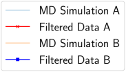
Figure 3: Filtering of MD simulation data with a uniform filter for a compression test along the $x$ axis. The filtering is performed twice for two MD simulations with different thermostat coupling parameters and thus different oscillations.

To examine whether the filter introduces significant bias to the filter data, we apply our filtering procedure to two MD simulations with the same strain path but initiated from different initial conditions. The filtered and unfiltered constitutive responses are compared for both cases, as shown in Fig. 3. The two MD simulations demonstrate different fluctuation patterns but the filtered responses are very close The uniform filter used to process the data appears to capture almost identical behaviors for both simulations.

3 Finite strain hyperelastic neural network functional for $\beta$-HMX

In this work, we will approximate a finite strain hyperelastic energy functional for $\beta$-HMX using a feed-forward neural network architecture trained with a modified Sobolev training loss function that incorporates additional physical constraints via a transfer learning technique. The following assumptions and setup have been made:

1. There exists one stress-free configuration for the $\beta$-HMX for which the stored elastic energy is zero. This configuration constitutes the reference configuration for the deformation mapping.

2. We assume that all the data used in the training are purely elastic with no path dependence.

3. Thermo-mechanical and rate-dependence effects on the elasticity are neglected.

4. A filter is used to reduce the high-frequency responses.

The stored energy functional $\bar{\psi}$ can be written as a function of the deformation gradient $\boldsymbol{F}$. The first Piola-Kirchhoff stress $\boldsymbol{P}$ is conjugate to the deformation gradient $\boldsymbol{F}$ and can be obtained from the following relation,

$$\boldsymbol{P}(\boldsymbol{F})=\frac{\partial\bar{\psi}(\boldsymbol{F})}{\partial\boldsymbol{F}}.$$ (2)

Notice that a necessary condition for this energy functional to be correct is the material-frame indifference. Here the deformation gradient is not sensitive to rigid-body translation. However, to ensure the the $SO(3)$ equivalence, the machine learning generated energy functional must satisfy the following constraint,

$$\bar{\psi}(\boldsymbol{F})=\bar{\psi}(\boldsymbol{QF}),\quad\forall\boldsymbol{Q}\in SO(3)$$ (3)

A possible way to bypass the need to introduce additional constraints in the loss function is to to derive the energy functional as a function of the Green strain tensor $\boldsymbol{E}$ for which:

$$\boldsymbol{E}^{\prime}=\frac{1}{2}(\boldsymbol{C}^{\prime}-\boldsymbol{I})=\frac{1}{2}(\boldsymbol{F}^{\prime T}\cdot\boldsymbol{F}^{\prime}-\boldsymbol{I})=\frac{1}{2}(\boldsymbol{F}^{T}\cdot\boldsymbol{Q}^{T}\cdot\boldsymbol{Q}\cdot\boldsymbol{F}-\boldsymbol{I})=\frac{1}{2}(\boldsymbol{F}^{T}\cdot\boldsymbol{F}-\boldsymbol{I})=\frac{1}{2}(\boldsymbol{C}-\boldsymbol{I})=\boldsymbol{E},$$ (4)

so we then acquire an equivalent expression:

$$\bar{\psi}(\boldsymbol{F})=\psi(\boldsymbol{E}).$$ (5)

The second Piola-Kirchhoff stress $\boldsymbol{S}$ is conjugate to the Green strain $\dot{\boldsymbol{E}}$, which is derived as:

$$\boldsymbol{S}(\boldsymbol{E})=\frac{\partial\psi(\boldsymbol{E})}{\partial\boldsymbol{E}}.$$ (6)

In addition to the frame invariance, another major benefit of expressing the energy functional in terms of the Green strain tensor is that the resultant stress measure is symmetric and the elastic tangential operator possesses both major and minor symmetries. These symmetries may reduce the dimension of the input parametric space 9 to 6 and hence simplify the training. Furthermore, while $\boldsymbol{C}$ and $\boldsymbol{E}$ can both be used as the input for the inherently frame-indifferent energy functional that yields $\boldsymbol{S}$ as the first derivative, $\boldsymbol{E}=\boldsymbol{0}$ implies the energy functional becomes zero. Meanwhile, training $\bar{\psi}(\boldsymbol{F})$ as the learned function can be more convenient for implicit PDE solver for large deformation where the tangent corresponding to $\boldsymbol{P}-\boldsymbol{F}$ is required to solve the linearized system of equation.

As such, we will train two hyperelasticity functionals, one takes the deformation gradient as input and another one takes the Green strain tensor as input respectively and we will compare the results obtained from numerical experiments. The relationships among elasticity tangential tensors corresponding to different stress-strain conjugate pairs will also be discussed in Section 5.

4 Stress-based Sobolev training for stored-energy function

We introduce a neural network training technique that constructs the hyperelasticity energy functional using solely the stress data and a single reference configuration where $\boldsymbol{F}=\boldsymbol{I}$. Recall that a feed-forward neural network can be trained to approximate an energy functional $\psi$ that takes the Green-Lagrange deformation tensor $\boldsymbol{E}$ as input. This energy function is parametrized by weights $\boldsymbol{W}$ and biases $\boldsymbol{b}$. The supervised learning that minimizes the inner product of the difference between the true $\psi$ and the approximated $\hat{\psi}$ for $N$ samples can be written as

$$W^{\prime},b^{\prime}=\underset{W,b}{\operatorname{argmin}}\left(\frac{1}{N}\sum_{i=1}^{N}\left\|\psi_{i}-\hat{\psi}_{i}\right\|_{2}^{2}\right),$$ (7)

where $\psi_{i}=\psi(\boldsymbol{E}_{i})$ and $\hat{\psi}_{i}=\hat{\psi}(\boldsymbol{E}_{i})$ accordingly. While this approach could reduce the discrepancy of the predicted and true free energy values—if available, it would not necessarily improve the performance of the stress predictions. However, true energy functional value samples were not available from the MD simulations, thus, we designed a variation of the free energy functional loss function that only uses stress data. From this point forward, we refer to free energy simply as energy.

4.1 Sobolev constraints for the hyperelastic energy functional

To introduce a hyperelasticity model suitable to incorporate into numerical solvers for boundary value problems, the accuracy, stability, robustness, smoothness, and uniqueness of the hyperelasticity responses are all important to consider. Unlike neural networks that directly generate stress predictions, a hyperelasticity model must be sufficiently smooth and differentiable to avoid discontinuity in the predicted stress and elastic tangent (vlassis2020geometric; vlassis2021sobolev; le2015computational).

Consider the stored-energy functional solely constructed via (1) a reference configuration where the Green strain tensor equals to $\boldsymbol{E}_{0}$, and (2) the Cauchy stress measured in the MD simulations. The corresponding loss function reads,

$$W^{\prime},b^{\prime}=\underset{\boldsymbol{W},b}{\operatorname{argmin}}\left(\left\|\psi_{0}-\hat{\psi}_{0}\right\|_{2}^{2}+w_{\boldsymbol{S}}\left\|\frac{\partial\psi_{0}}{\partial\boldsymbol{E}_{0}}-\frac{\partial\hat{\psi}_{0}}{\partial\boldsymbol{E}_{0}}\right\|_{2}^{2}+\frac{w_{\boldsymbol{S}}}{N}\sum_{i=1}^{N}\left\|\frac{\partial\psi_{i}}{\partial\boldsymbol{E}_{i}}-\frac{\partial\hat{\psi}_{i}}{\partial\boldsymbol{E}_{i}}\right\|_{2}^{2}\right),$$ (8)

where $\psi_{0}=\psi(\boldsymbol{E}_{0})$ and $\hat{\psi}_{0}=\psi(\boldsymbol{E}_{0})$ are the true and approximated values of the energy functional at strain $\boldsymbol{E}_{0}$, $N$ is the number of non-trivial stress data, and $w_{\boldsymbol{S}}$ is the weighting factor for the multi-objective optimization. In this work, we use the configuration at ($300\text{\,}\mathrm{K}$, $1\text{\,}\mathrm{a}\mathrm{t}\mathrm{m}$) as the reference and assume this configuration is stress-free.

The corresponding loss function for the energy conjugate pair $\boldsymbol{P}-\boldsymbol{F}$ hyperelastic model is:

$$W^{\prime},b^{\prime}=\underset{\boldsymbol{W},b}{\operatorname{argmin}}\left(\left\|\psi_{0}-\hat{\psi}_{0}\right\|_{2}^{2}+w_{\boldsymbol{P}}\left\|\frac{\partial\psi_{0}}{\partial\boldsymbol{F}_{0}}-\frac{\partial\hat{\psi}_{0}}{\partial\boldsymbol{F}_{0}}\right\|_{2}^{2}+\frac{w_{\boldsymbol{P}}}{N}\sum_{i=1}^{N}\left\|\frac{\partial\psi_{i}}{\partial\boldsymbol{F}_{i}}-\frac{\partial\hat{\psi}_{i}}{\partial\boldsymbol{F}_{i}}\right\|_{2}^{2}\right),$$ (9)

where $\psi_{0}=\psi(\boldsymbol{F}_{0})$ and $\hat{\psi}_{0}=\psi(\boldsymbol{F}_{0})$ are the true and approximated values of the energy functional at the reference configuration $\boldsymbol{F}_{0}$ at ($300\text{\,}\mathrm{K}$, $1\text{\,}\mathrm{a}\mathrm{t}\mathrm{m}$).

4.2 Transfer learning to enforce frame invariance

A hyperelastic model described by the conjugate pair $\boldsymbol{P}-\boldsymbol{F}$ tensors is expected to satisfy the frame invariance conditions described in Eq. (3). To ensure that the frame invariance is preserved during training, we re-use a previously trained neural network but modifying the loss function by introducing a number $M$ of random rotations $\boldsymbol{Q}^{m},i=1,2,...,M$ and penalizing the violation of the objectivity by adding the following weighted objectives:

$$\begin{split}w_{\psi}\frac{1}{M}\sum_{m=1}^{M}\left\|\psi(\boldsymbol{Q}^{m}\boldsymbol{F})-\psi(\boldsymbol{F})\right\|+w_{\boldsymbol{P}}\frac{1}{M}\sum_{m=1}^{M}\left\|\boldsymbol{P}(\boldsymbol{Q}^{m}\boldsymbol{F})-\boldsymbol{Q}^{m}\boldsymbol{P}(\boldsymbol{F})\right\|_{2}^{2}\\ +w_{\mathbb{C}}\frac{1}{M}\sum_{m=1}^{M}\left\|\boldsymbol{A}(\boldsymbol{Q}^{m}\boldsymbol{F})-\boldsymbol{Q}^{m}\boldsymbol{Q}^{m}\boldsymbol{A}(\boldsymbol{F})\right\|_{F}^{2}.\end{split}$$ (10)

4.3 Transfer learning to enforce crystal symmetries

The monoclinic unit cell of the single crystal $\beta$-HMX in the $P2_{1}/n$ space group setting is shown in Figure 4. The covariant crystal basis vectors $\boldsymbol{M}_{1}$, $\boldsymbol{M}_{2}$, and $\boldsymbol{M}_{3}$ represent the crystal axis in the reference configuration, with corresponding contravariant basis vectors $\boldsymbol{M}^{1}$, $\boldsymbol{M}^{2}$, and $\boldsymbol{M}^{3}$ such that $\boldsymbol{M}^{i}\cdot\boldsymbol{M}_{j}=\delta^{i}_{j}$. Furthermore, the covariant crystal basis vectors in the current configuration are denoted as $\boldsymbol{m}_{1}$, $\boldsymbol{m}_{2}$, and $\boldsymbol{m}_{3}$, where $\boldsymbol{m}_{i}=\boldsymbol{F}\boldsymbol{M}_{i}$. A general form of the deformation gradient $\boldsymbol{F}$ that maintains the monoclinic unit cell reads:

$$V_{F}=\{\boldsymbol{F}|\boldsymbol{F}=\boldsymbol{RU},\boldsymbol{U}=\sum_{i=1}^{3}(a_{i}\boldsymbol{M}_{i}\otimes\boldsymbol{M}^{i})+a_{4}(\boldsymbol{M}_{1}\otimes\boldsymbol{M}^{3}+\boldsymbol{M}_{3}\otimes\boldsymbol{M}^{1}),\boldsymbol{R}\in\textrm{SO(3)},a_{j}\in\mathbb{R}\}.$$ (11)

Figure 4: Monoclinic unit cell of $\beta$-HMX in the $P2_{1}/n$ space group setting. The lattice constants are $a=$6.53\text{\,}\mathrm{\SIUnitSymbolAngstrom}$$, $b=$11.03\text{\,}\mathrm{\SIUnitSymbolAngstrom}$$, $c=$7.35\text{\,}\mathrm{\SIUnitSymbolAngstrom}$$, $\alpha=\gamma=$90\text{\,}\mathrm{\SIUnitSymbolDegree}$$, and $\beta=$102.689\text{\,}\mathrm{\SIUnitSymbolDegree}$$ (at $295\text{\,}\mathrm{K}$) (eiland1954crystal). The vectors $\boldsymbol{e}_{1}$, $\boldsymbol{e}_{2}$, and $\boldsymbol{e}_{3}$ denote the basis vectors of the global Cartesian coordinate system.

Under an imposed deformation gradient under the constraint in Equation (11), the symmetry group of the monoclinic unit cell in the current configuration reads

$$V_{Q}=\{\boldsymbol{Q}|\boldsymbol{Q}=\exp\left[k\pi\frac{\operatorname{spn}(\boldsymbol{m}_{2})}{\|\boldsymbol{m}_{2}\|}\right],\quad\boldsymbol{m}_{2}=\boldsymbol{F}\boldsymbol{M}_{2},\quad\boldsymbol{F}\in V_{F},\quad k\in\mathbb{Z}\}.$$ (12)

Here, the infinitesimal rotation map and the finite rotation map are defined as (simo1989stress)

$$\operatorname{spn}(\boldsymbol{\theta})=-\boldsymbol{\varepsilon}\cdot\boldsymbol{\theta},\quad\exp\left[\operatorname{spn}(\boldsymbol{\theta})\right]=\boldsymbol{I}+\frac{\sin(\theta)}{\theta}\operatorname{spn}(\boldsymbol{\theta})+\frac{1-\cos(\theta)}{\theta^{2}}\operatorname{spn}(\boldsymbol{\theta})^{2},$$

where $\boldsymbol{\varepsilon}$ is the permutation tensor and $\theta=\|\boldsymbol{\theta}\|$ is the rotation angle.

Due to material symmetry, the first elasticity tensor $\mathbb{C}^{PF}$ has the following symmetric property:

$$\mathbb{C}^{PF}(\boldsymbol{F\boldsymbol{Q}})=\mathbb{C}^{PF}(\boldsymbol{F}),\quad\forall\boldsymbol{F}\in V_{F},\boldsymbol{Q}\in V_{Q},$$ (13)

where the tensor components are expressed in the global Cartesian frame for convenience.

To ensure that the crystal symmetry is preserved, we can again re-use the previous trained function (9) and (10), and modify the loss function by introducing $M$ number of rotations $\boldsymbol{Q}^{k}_{\text{sym}}\in V_{Q},k=1,2,...,M$ to penalize the violation of the material symmetry by adding the following weighted objectives:

$$\begin{split}\sum_{k=1}^{M}\left(w_{\psi}\frac{1}{N}\sum_{i=1}^{N}\left\|\psi(\boldsymbol{F}\boldsymbol{Q}^{k}_{\text{sym}})-\psi(\boldsymbol{F})\right\|+w_{\boldsymbol{P}}\frac{1}{N}\sum_{i=1}^{N}\left\|\boldsymbol{P}(\boldsymbol{F}\boldsymbol{Q}^{k}_{\text{sym}})-\boldsymbol{P}(\boldsymbol{F})\boldsymbol{Q}^{k}_{\text{sym}}\right\|_{2}^{2}\right.\\ \left.+w_{\mathbb{C}}\frac{1}{N}\sum_{i=1}^{N}\left\|\boldsymbol{A}(\boldsymbol{F}\boldsymbol{Q}^{k}_{\text{sym}})-\boldsymbol{A}(\boldsymbol{F})\boldsymbol{Q}^{k}_{\text{sym}}\boldsymbol{Q}^{k}_{\text{sym}}\right\|_{F}^{2}\right).\end{split}$$ (14)

5 Post-training validation of the predicted elastic tangential operators

In this section, we introduce numerical tests to determine whether the predicted constitutive responses are thermodynamically admissible, preserve the symmetry, and lead to unique and stable elastic responses. A subset of these criteria are required to constitute a correct constitutive law (e.g. material frame invariance), while others such as the convexity and the strong ellipticity are not necessary conditions but are desirable properties for stability and uniqueness of the boundary value problem. While in principle many of these physics constraints/laws can be incorporated into the loss function in the supervised learning process, putting all the constraints explicitly into the loss function is not necessarily always ideal, as the multiple constraints may alter the landscape of the loss function and thus complicate the search for the optimal energy functional (mavrotas2009effective).

As such, our goal is to introduce a suite of necessary conditions which the learned hyperelasticity constitutive law must fulfill. These necessary conditions, along with the fact that the hyperleasticity constitutive law must be capable of generating predictions within a threshold error, are necessary but not sufficient to guarantee the safety of using the machine learning model for high-consequence high-risk predictions (such as those for explosives).

5.1 Mapping between finite and infinitesimal kinematics

To examine the admissibility of the hyperelasticity model and compare the finite strain model with other published results based on the infinitesimal strain assumption, the connections among the tangents of different energy-conjugate pairs are provided below for completeness. Here our first goal is to obtain an underlying small-strain tangent of the finite-strain counterpart by using the logarithmic and exponential mappings, such that the elasticity tensors predicted here and those from the literature can be compared. Recall that the logarithmic elastic strain $\boldsymbol{\epsilon}$ can be defined as (cuitino1992material),

$$\boldsymbol{\epsilon}=\ln\boldsymbol{U}^{2}=\frac{1}{2}\ln\boldsymbol{C},\quad,$$ (15)

where $\boldsymbol{U}$ is the right-stretch tensor and $\boldsymbol{C}$ is the right Cauchy-Green strain tensor. The small-strain elastic tensor $\mathbb{C}^{\boldsymbol{\sigma}-\boldsymbol{\epsilon}}$ can be obtained from the chain rule,

$$\mathbb{C}^{\boldsymbol{\sigma}-\boldsymbol{\epsilon}}=\frac{\partial\boldsymbol{\sigma}}{\boldsymbol{\partial\epsilon}}=\frac{\partial\boldsymbol{\sigma}}{\partial\boldsymbol{S}}:\frac{\partial\boldsymbol{S}}{\partial\boldsymbol{E}}:\frac{\partial\boldsymbol{E}}{\partial\boldsymbol{\epsilon}}=\frac{1}{2}\frac{\partial\boldsymbol{\sigma}}{\partial\boldsymbol{S}}:\frac{\partial\boldsymbol{S}}{\partial\boldsymbol{E}}:\frac{\partial\boldsymbol{C}}{\partial\boldsymbol{\epsilon}}=\frac{1}{2}\frac{\partial\boldsymbol{\sigma}}{\partial\boldsymbol{S}}:\frac{\partial\boldsymbol{S}}{\partial\boldsymbol{E}}:\frac{\partial\exp\boldsymbol{2\epsilon}}{\partial\boldsymbol{\epsilon}},$$ (16)

where $\boldsymbol{\sigma}=J^{-1}\boldsymbol{F}\cdot\boldsymbol{S}\cdot\boldsymbol{F}^{T}$ is the Cauchy stress. To compute the small-strain elasticity tensor, one first rewrites Eq. (15) in an infinite series representation,

$$\boldsymbol{C}=\exp 2\boldsymbol{\epsilon}=\sum^{\infty}_{n=0}\frac{1}{n!}(2\boldsymbol{\epsilon})^{n}.$$ (17)

As such, the Cartesian component of the derivative $\partial\boldsymbol{C}/\partial{\boldsymbol{\epsilon}}$ reads (miehe1998comparison)

$$[\frac{\partial\boldsymbol{C}}{\partial\boldsymbol{\epsilon}}]_{ijkl}=\sum^{\infty}_{n=1}\frac{2^{n}}{n!}\sum^{\infty}_{m=1}[\boldsymbol{\epsilon}^{m-1}_{ik}][\boldsymbol{\epsilon}^{n-m}_{lj}].$$ (18)

The first tangential tensor $\mathbb{C}^{\boldsymbol{P}-\boldsymbol{F}}$ can be related to the second derivative of the hyperelastic energy functional $\psi(\boldsymbol{E})$,

$$\mathbb{C}^{\boldsymbol{P}-\boldsymbol{F}}=\frac{\partial\boldsymbol{P}}{\partial\boldsymbol{F}}=\frac{\partial\boldsymbol{S}}{\partial\boldsymbol{E}}\cdot\boldsymbol{F}\cdot\boldsymbol{F}\cdot\boldsymbol{g}+\boldsymbol{S}\otimes\boldsymbol{\delta},$$ (19)

where $\boldsymbol{g}$ is the metric tensor. This expression is derived from marsden1994mathematical (see page 215), where we simply use the chain rule to link the tangents $\partial\boldsymbol{S}/\partial\boldsymbol{E}$ with $\partial\boldsymbol{S}/\partial\boldsymbol{C}$. Note that this tensor corresponds to the first Piola-Kirchhoff stress and the deformation gradient, and does not possess minor symmetry.

In both Eq. (16) and Eq. (19), the derivative $\partial\boldsymbol{S}/\partial\boldsymbol{E}$ is obtained from the neural elastic stored energy, while the rest of the terms can be obtained via either analytical solution or automatic differentiation.

5.2 Strong ellipiticity

While many works are dedicated to training elastic constitutive laws (ghaboussi1998autoprogressive; pernot1999application; le2015computational; hoerig2018data; fuhg2021local; huang2020learning; vlassis2020geometric; vlassis2021sobolev), surprisingly few among these analyze the stability and uniqueness of the learned neural network constitutive laws or provide any evidence of the well-posedness for the trained model. Recent work by (klein2021polyconvex) address this issue by enforcing polyconvexity via invariants (cf. hartmann2003polyconvexity).

Consider $\boldsymbol{A}$ to be the acoustic tensor corresponding to $\mathbb{C}^{PF}$ and that $\mathbb{C}^{PF}$ is the elastic tangential operator for the energy conjugate pairs $(\boldsymbol{P},\boldsymbol{F})$, that is,

$$\boldsymbol{A}(\boldsymbol{N})=\boldsymbol{N}\cdot\mathbb{C}^{PF}\cdot\boldsymbol{N}$$ (20)

The Legendre-Hadamard condition requires that for any pair of vectors $\boldsymbol{N}$ and $\boldsymbol{m}$, the following condition holds:

$$\boldsymbol{m}\cdot\boldsymbol{A}\cdot\boldsymbol{m}\geq 0,$$ (21)

where $\boldsymbol{N}$ is a Lagrangian unit vector and $\boldsymbol{m}$ is an Eulerian vector. Because we assume that $\beta$-HMX is a Green-elastic material, the necessary and sufficient conditions for strong ellipticity are (cf. ogden1997non page 392)

$$A_{ii}(\boldsymbol{N}) > 0,\quad i\in\{1,2,3\}$$ (22)

$$A_{ii}(\boldsymbol{N})A_{jj}(\boldsymbol{N})-A_{ij}(\boldsymbol{N})^{2} > 0,\quad j\neq i\in\{1,2,3\}$$ (23)

$$\det A(\boldsymbol{N}) > 0$$ (24)

for any $\boldsymbol{N}\in\mathbb{R}^{3}$. Notice that the material response is nonlinear and the ellipticity may vary according to the Eulerian vector $\boldsymbol{m}$. A simple way to ensure the conditions (22)-(24) are satisfied is to create the worst-case scenario, that is, find the infimum, and the unit vectors $\boldsymbol{N}$ that minimize $A_{ii}(\boldsymbol{N})$, $A_{ii}(\boldsymbol{N})A_{jj}(\boldsymbol{N})-A_{ij}(\boldsymbol{N})^{2}$, and $\det A(\boldsymbol{N})$ accordingly and check whether the three terms remain positive. Depending on the parameterization, the corresponding minimization problems can be written as

$$f(q) = A_{ii}(\boldsymbol{N}(q)),\quad\underset{q}{\operatorname{argmin}}\;f(q),\quad\boldsymbol{N}(q)\in S^{2}$$ (25)

$$g(q) = A_{ii}(\boldsymbol{N}(q))A_{jj}(\boldsymbol{N}(q))-A_{ij}(\boldsymbol{N}(q))^{2},\quad\underset{q}{\operatorname{argmin}}\;g(q),\quad\boldsymbol{N}(q)\in S^{2}$$ (26)

$$d(q) = \det A(\boldsymbol{N}(q)),\quad\underset{q}{\operatorname{argmin}}\;d(q),\quad\boldsymbol{N}(q)\in S^{2},$$ (27)

where $q$ represents a parametrization of the unit vector $\boldsymbol{N}(q)$. mota2016cartesian provide a comprehensive review of how different parameterizations, namely the spherical, stereographic, projective and tangent parameterizations, may lead to different local mininizers of the acoustic tensor in the parametric space. For spherical parameterization, a unit vector $\boldsymbol{N}$ is an element of the unit sphere $S^{2}$ which can be parameterized by the spherical coordinates, that is, the polar angle $\phi\in[0,\pi]$ and the azimuthal angle $\theta\in[0,\pi]$:

$$\boldsymbol{N}(\phi,\theta)=\sin\phi\cos\theta\boldsymbol{e}_{1}+\sin\phi\sin\theta\boldsymbol{e}_{2}+\cos\phi\boldsymbol{e}_{3},$$ (28)

where $\{\boldsymbol{e}_{1},\boldsymbol{e}_{2},\boldsymbol{e}_{3}\}$ is the the orthogonal basis for $\mathbb{R}^{3}$.

To ensure stability for any given admissible deformation, we must ensure that Eqs. (22)-(24) are valid for any $\boldsymbol{F}$. While this can be, in principle, determined analytically for hand-crafted energy functionals, the expression of the neural network energy functional would likely be too complicated to analyze. As such, we again resort to constructing a test to check the hypothesis that the material demonstrates strongly ellicipticity, via an attempt to find the minima, that is,

$$f^{\prime}(q,\boldsymbol{F}) = A_{ii}(\boldsymbol{N}(q),\boldsymbol{F}),\quad\underset{q,\boldsymbol{F}}{\operatorname{argmin}}\;f^{\prime}(q,\boldsymbol{F}),\quad\boldsymbol{N}(q)\in S^{2},\boldsymbol{F}\in GL^{+}(3)$$ (29)

$$g^{\prime}(q,\boldsymbol{F}) = A_{ii}(\boldsymbol{N}(q),\boldsymbol{F})A_{jj}(\boldsymbol{N}(q),\boldsymbol{F})-A_{ij}(\boldsymbol{N}(q),\boldsymbol{F})^{2},\quad$$ (30)

$$\underset{q,\boldsymbol{F}}{\operatorname{argmin}}\;g^{\prime}(q),\quad\boldsymbol{N}(q)\in S^{2},\boldsymbol{F}\in GL^{+}(3)$$

$$d^{\prime}(q,\boldsymbol{F}) = \det A(\boldsymbol{N}(q),\boldsymbol{F}),\quad\underset{q,\boldsymbol{F}}{\operatorname{argmin}}\;d^{\prime}(q,\boldsymbol{F}),\quad\boldsymbol{N}(q)\in S^{2},\boldsymbol{F}\in GL^{+}(3).$$ (31)

It is impossible to test all the possible deformation gradients in the MD simulations while maintaining the path independence of the constitutive responses, so we instead construct a test where we only consider a range of possible deformation gradients and search for the minima within this range.

The numerical strong ellipticity test is conducted via the following three steps.

1. We create two sets of point clouds in the parametric space with uniform spacing, $V_{q}=\{q_{1},q_{2},q_{3},....\}$ and $V_{\boldsymbol{F}}=\{\boldsymbol{F}_{1},\boldsymbol{F}_{2},\boldsymbol{F}_{3},...\}$, and select the combination of $(q,\boldsymbol{F})$ that minimizes $f^{\prime}$, $g^{\prime}$, $d^{\prime}$. If there exist other $(q,\boldsymbol{F})$ combinitions that yield a value sufficiently close to the minimum (say within 5% difference), then the additional coordinates will be stored as the candidate position(s) for the gradient-free search. This treatment is to ensure that more local optimal points can be identified and compared and to avoid the issues exhibited in mota2016cartesian.

2. We then use the candidate position determined from the previous step as the starting point and apply a gradient-free optimizer via the third-party gradient-free optimizer library (cf. gfo2020) to examine whether we can find new coordinates for which the functions $f^{\prime}(q,\boldsymbol{F})$, $g^{\prime}(q,\boldsymbol{F})$, and $d^{\prime}(q,\boldsymbol{F})$ are smaller than the candidate position(s) identified in Step 1.

3. If Eqs. (22) - (24) are not violated in the worst case obtained from the Step 2, then we consider the neural network functional to have passed the strong ellipticity test.

5.3 Convexity and growth conditions

In nonlinear elasticity in the finite strain regime, convexity is not necessary and can be over-restrictive for physical phenomena that involve instability or buckling (clayton2010nonlinear). Nevertheless, the convexity condition has to be satisfied to predict stable elastic responses under large deformation. The convexity condition can be stated as (cf. (ogden1997non)),

$$\psi(\boldsymbol{F}^{\prime})-\psi(\boldsymbol{F})-\operatorname{tr}(\boldsymbol{P}\cdot(\boldsymbol{F}-\boldsymbol{F}^{\prime}))\geq 0$$ (32)

Because convexity is not a requirement for realistic simulations (although it might be expected for HMX), we do not incorporate this criterion in the training of the neural network. However, the uniqueness and stability of the elasticity model are not only important for predicting realistic elastic responses but crucial if the model will be deployed as the underlying elasticity model for crystal plasticity and damage models.

Another important condition to prevent degenerated elastic behavior is from rosakis1994relation which requires

$$\psi(\boldsymbol{F})\rightarrow\infty\quad\text{as}\quad\det\boldsymbol{F}\rightarrow 0^{+}.$$ (33)

Recall that $\det\boldsymbol{F}\rightarrow 0$ only happen if the distance between two material points that was non-zero in the reference configuration vanishes in the current configuration. Note that it is unlikely a material would remain elastic if the volumetric deformation is extremely large. furthermore, enforcing these constraints explicitly in the loss function is difficult due to the infinity. Nevertheless, the constraint may provide a helpful indicator of the admissibility of the machine learning extrapolated predictions. As a result, we suggest a post-training validation test where we generate the response for deformation gradients with $\det\boldsymbol{F}$ approaching zero and observe whether the resultant energy is monotonically increasing.

5.4 Material Anisotropy

A predictive elasticity model must preserve the overall crystal symmetry while capturing how the anisotropy of the elasticity tensor evolves under arbitrary deformation. The degree of anisotropy of the elastic response can be measured by various metrics available in the literature (cf. (li1987single; kube2016elastic; ranganathan2008universal)). Many of these anisotropy metrics (or indices) are intended for components of the elasticity tensor. Typically, the distinction between the secant and tangential elastic tensors is not taken into account. This can be confusing for materials undergoing finite deformation where both material and geometrical non-linearities play important roles in the anisotropy of the constitutive response. More importantly, the impacts of the former and latter types of non-linearity should be distinguished properly such that a meaningful evaluation can be conducted.

5.4.1 Ledbetter and Migliori general anisotropy index

Here, we use the idea from previous work due to ledbetter2006general, where the ratio between the maximum and minimum shear-wave speed is used to define an anisotropy measure. Interestingly, this method can also be used to detect instability as the vanishing of the slowest wave speed is accompanied by divergence of the Ledbetter-Migliori index.

This measure can be easily extended to the finite strain regime by replacing the infinitesimal elasticity tangent with the elasticity tensor corresponding to the first Piola-Kirchhoff stress and deformation gradient (ogden1997non). This idea can be summarized into the following steps.

1. Generate as many unit vectors $\boldsymbol{N}$ as possible.

2. Solve the Christoffel equation for each unit vector $\boldsymbol{N}$, that is,

   $$\det\left(\boldsymbol{N}\cdot\mathbb{C}(\boldsymbol{F})\cdot\boldsymbol{N}-\rho v^{2}\boldsymbol{I}\right)=0$$ (34)

3. Pick the largest solution $v_{2}$ and the smallest solution $v_{1}$. Then, the anistropy index is simply

   $$A_{I}=v_{2}^{2}/v_{1}^{2}$$ (35)

Here, instead of a Monte Carlo search, we can leverage the search formulated in Section 5.2 to obtain the smallest eigenvalue $v_{1}$ and largest eigenvalue $v_{2}$ of the acoustic tensor. Again, the optimization is conducted by using a uniformly spaced point cloud to search for the initial guess, then a gradient-free optimizer is used to find the normal vectors that maximize and minimize $v$.

6 Results

In this section, we discuss the performance of neural network models for discovering the hyperelastic energy functional from the $\beta$-HMX MD simulation data. We describe the training setup of the networks and compare the performance of the architectures. We then demonstrate the predictive capabilities of the models against the present MD simulation data and elastic constants taken from the literature for the same MD force field used here. Finally, we investigate the energy functional models in terms of how well they satisfy desired properties from the hyperelasticity literature.

6.1 Training performance and learning capacity

In this section, we discuss the performance of the neural network architectures for the Sobolev constraints described in Section 4. We first demonstrate how we trained the neural networks to generate a hyperelastic energy functional data from the MD simulation data. We use two different architectures to discover the hyperelastic energy functional for $\beta$-HMX. The first architecture is based on the energy conjugate pair $\boldsymbol{S}-\boldsymbol{E}$ (Model $\mathcal{M}_{1}$). The input and output variables are symmetric tensors and, thus, can be described by six components. The second architecture is based on the energy conjugate pair $\boldsymbol{P}-\boldsymbol{F}$ (Model $\mathcal{M}_{2}$). In addition, we also re-train Model $\mathcal{M}_{2}$ with an additional material frame indifference constraint (Eq. (10) )in the loss function (model $\mathcal{M}_{3}$). As the difference in the predictions obtained from Models $\mathcal{M}_{2}$ and $\mathcal{M}_{3}$ is minor, we did not enforce the Eq. (10) explicitly in the the last model we trained (Model $\mathcal{M}_{4}$). Instead, only monoclinic symmetry is enforced as an additional term for the weighted loss function in the re-training step to ensure that the material symmetry is preserved.

Table 2: Summary of the trained models.

Model	Description
$\mathcal{M}_{1}$	Energy conjugate pair $\boldsymbol{S}-\boldsymbol{F}$ model trained via the loss function described in Eq. 8.
$\mathcal{M}_{2}$	Energy conjugate pair $\boldsymbol{P}-\boldsymbol{F}$ model trained via the loss function described in Eq. 9.
$\mathcal{M}_{3}$	Energy conjugate pair $\boldsymbol{P}-\boldsymbol{F}$ model trained with pre-trained model $\mathcal{M}_{2}$ and additional loss function Eq. (10) to enforce material frame indifference.
$\mathcal{M}_{4}$	Energy conjugate pair $\boldsymbol{P}-\boldsymbol{F}$ model trained pre-trained model $\mathcal{M}_{2}$ and additional loss function Eq. (14) to enforce monoclinic symmetry.

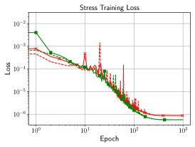
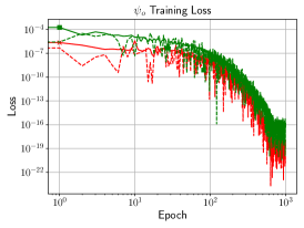
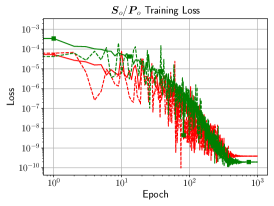
(a)	(b)	(c)

Figure 5: Comparison of the training loss curves for the energy conjugate pair $\boldsymbol{S}-\boldsymbol{E}$ model ($\mathcal{M}_{1}$) and the energy conjugate pair $\boldsymbol{P}-\boldsymbol{F}$ model ($\mathcal{M}_{2}$) for (a) the stress, (b) the energy, and (c) stress value at the state of zero strain.

The energy functional neural networks have a feed-forward architecture consisting of a hidden dense layer (100 neurons / ReLU), followed by two multiply layers (cf. vlassis2021sobolev), then another hidden dense layer (100 neurons / ReLU), and finally an output dense layer (Linear). The training and validation procedures of the neural network are implemented in Python with machine learning libraries Keras (chollet2015keras) and Tensorflow (tensorflow2015). The kernel weight matrix of the layers was initialized with a Glorot uniform distribution and the bias vector with a zero distribution. The models were trained on 163400 MD simulation data points and validated on 70030 data points. All the models were trained for 1000 epochs with a batch size of 512, using the Nadam optimizer (dozat2016incorporating) initialized with default values in the Keras library.

The loss function training curves for the architectures $\mathcal{M}_{1}$ and $\mathcal{M}_{2}$ are demonstrated in Fig. 5. The two architectures appear to have similar accuracy so they will be used interchangeably below. The predictive capabilities of $\mathcal{M}_{1}$ and $\mathcal{M}_{2}$ are further demonstrated in Section 6.2.1.

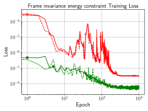
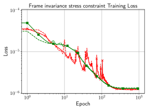
(a)	(b)

Figure 6: Comparison of the training loss curves for (a) the energy and (b) stress frame invariance constraints for the energy conjugate pair $\boldsymbol{P}-\boldsymbol{F}$ model ($\mathcal{M}_{2}$) without any additional constraints in the loss function and the energy conjugate pair $\boldsymbol{P}-\boldsymbol{F}$ model ($\mathcal{M}_{3}$) trained with the additional frame invariance constraint loss function Eq. (10).

To check and, if necessary, enforce the frame invariance of the neural network hyperelastic models as described in Section 4.2, we conduct a transfer learning experiment by retraining the neural network model $\mathcal{M}_{2}$. We first train the energy conjugate pair $\boldsymbol{P}-\boldsymbol{F}$ model ($\mathcal{M}_{2}$) for 1000 epochs without any frame invariance constraints in the loss function (i.e., Eq. (9)). We record the frame invariance metrics during training by applying random rotation $\boldsymbol{Q}$ tensors on the input deformation gradient tensors and examine whether the material response is frame invariant; that is, whether the predicted energy remains the same before and after rotation and whether the predicted stress tensor rotates accordingly. The trained model $\mathcal{M}_{2}$ is then retrained with the additional frame invariance constraints in Eq. (10) for another 1000 epochs (model $\mathcal{M}_{3}$). The comparison of the training curves for $\mathcal{M}_{2}$ and $\mathcal{M}_{3}$ is shown in Fig. 6. Model $\mathcal{M}_{2}$ appears to already satisfy well the frame invariant properties, with the additional constraints of model $\mathcal{M}_{3}$ mostly improving the frame invariance energy constraints.

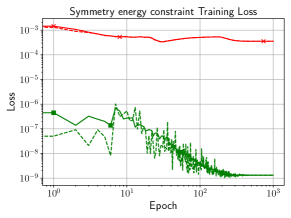
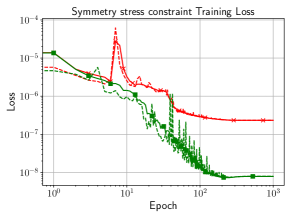
(a)	(b)

Figure 7: Comparison of the training loss curves for (a) the energy and (b) stress symmetry constraints for the energy conjugate pair $\boldsymbol{P}-\boldsymbol{F}$ model ($\mathcal{M}_{2}$) without any symmetry constraints in the loss function and the energy conjugate pair $\boldsymbol{P}-\boldsymbol{F}$ model ($\mathcal{M}_{4}$) trained with the additional symmetry-constraint loss function Eq. (14).

We also perform a transfer learning experiment by retraining the neural network model $\mathcal{M}_{2}$ to ensure it retains the observed $\beta$-HMX crystal symmetries as described in Section 4.3. We first train the energy conjugate pair $\boldsymbol{P}-\boldsymbol{F}$ model ($\mathcal{M}_{2}$) for 1000 epochs without any symmetry constraints in the loss function and record the symmetry metrics during training. By applying a rotation $\boldsymbol{Q}_{\text{sym}}$ on the input deformation gradient tensors, we check for the material response to retain the expected monoclinic symmetry behavior. The check includes the constraints up to the first-order derivatives of the network. The trained model $\mathcal{M}_{2}$ is then retrained with the additional symmetry constraints in Eq. (14) for another 1000 epochs (model $\mathcal{M}_{4}$). The results for the two training experiments are shown in Fig. 7, where the additional symmetry constraints appear to be improving both the energy and the stress symmetry constraints.

Remark 1.

Rescaling of the training data. As a pre-processing step, we have normalized all data to avoid the vanishing or exploding gradient problem that may occur during the back-propagation process (bishop1995neural). The $X_{i}$ sample of a measure $X$ is scaled to a unit interval via,

$$\overline{X_{i}}:=\frac{X_{i}-X_{\text{min}}}{X_{\text{max}}-X_{\text{min}}},$$ (36)

where $\overline{X_{i}}$ is the normalized sample point. $X_{\text{min}}$ and $X_{\text{max}}$ are the minimum and maximum values of the measure $X$ in the training data set such that all different types of data used in this paper (e.g. strain, stress, etc) are all normalized within the range $[0,1]$.

6.2 Validation of the constitutive responses

In this section, we validate the neural network predicted constitutive response against MD simulation data as well as $\beta$-HMX elastic coefficients from the literature. We also monitor the learned physical properties for the trained models, such as the strong ellipticity, the energy growth, and the anisotropy index.

6.2.1 Validation against unseen MD simulations

We validate the predictive performance of the learned models against unseen MD simulation loading paths. The neural network architectures considered in this section are the energy conjugate pair $\boldsymbol{S}-\boldsymbol{E}$ model ($\mathcal{M}_{1}$) and the energy conjugate pair $\boldsymbol{P}-\boldsymbol{F}$ model ($\mathcal{M}_{2}$).

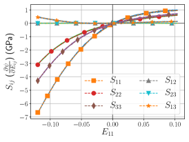
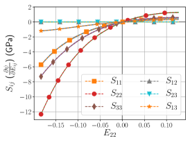
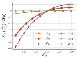
(a)	(b)	(c)

Figure 8: Comparison of the predicted stress response against three uniaxial MD simulations for the energy conjugate pair $\boldsymbol{S}-\boldsymbol{E}$ model ($\mathcal{M}_{1}$). (a) Uniaxial compression and extension along the $x_{1}$ axis. (b) Uniaxial compression and extension along the $x_{2}$ axis. (c) Uniaxial compression and extension along the $x_{3}$ axis.

.

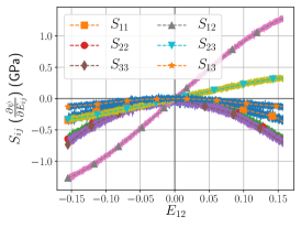
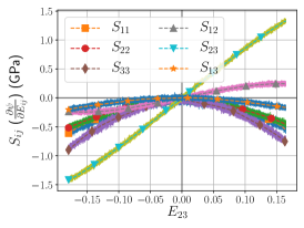
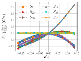
(a)	(b)	(c)

Figure 9: Comparison of the predicted stress response against three shear MD simulations for the energy conjugate pair $\boldsymbol{S}-\boldsymbol{E}$ model ($\mathcal{M}_{1}$). (a) Shear tests for positive and negative directions along the $\boldsymbol{e}_{1}\otimes\boldsymbol{e}_{2}$ direction. (b) Shear tests for positive and negative directions along the $\boldsymbol{e}_{2}\otimes\boldsymbol{e}_{3}$ direction. (c) Shear tests for positive and negative directions along the $\boldsymbol{e}_{1}\otimes\boldsymbol{e}_{3}$ direction.

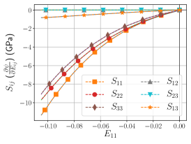
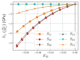
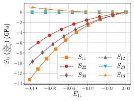
(a)	(b)	(c)

Figure 10: Comparison of the predicted stress response against three biaxial MD simulations for the energy conjugate pair $\boldsymbol{S}-\boldsymbol{E}$ model ($\mathcal{M}_{1}$). (a) Biaxial compression along the $x_{1}$ and $x_{2}$ axes. (b) Biaxial compression along the $x_{2}$ and $x_{3}$ axes. (c) Biaxial compression along the $x_{1}$ and $x_{3}$ axes.

The stress predictions of the networks against three uniaxial strains along the axes $x_{1}$, $x_{2}$, and $x_{3}$ are demonstrated in Fig. 8 and Fig. 11. All the symmetric stress tensor components are plotted against the main loading direction of the MD simulation experiment. The predictions are compared against the raw MD simulation data before the filtering pre-processing described in Section 2.4. The stress predictions for three pure shear MD experiments in the positive and negative $\boldsymbol{e}_{1}\otimes\boldsymbol{e}_{2}$, $\boldsymbol{e}_{2}\otimes\boldsymbol{e}_{3}$, and $\boldsymbol{e}_{1}\otimes\boldsymbol{e}_{3}$ directions are shown in Fig. 9 and Fig. 12. Finally, the stress predictions for three biaxial compression tests along the $x_{1}$ and $x_{2}$, $x_{2}$ and $x_{3}$, and $x_{1}$ and $x_{3}$ axes are shown in Fig. 10 and Fig. 13. It is noted that the stress fluctuations in the MD shear data appear to have a larger magnitude than those of the axial simulations. However, the magnitude of the fluctuations of the stress components is similar across all simulations; it appears to be larger in the shear simulations due to the smaller scale of the stress response.

Both models are able to accurately capture the shear behavior of $\beta$-HMX, which differs greatly in the positive vs. negative directions as seen in Fig. 9 and Fig. 12. The shear stress response of the material appears to be highly non-linear and exhibits directional dependence. This behavior is not expected to be captured by a material model with an invariant formulation, as it requires specific treatment of the shear response along different directions to replicate the directional dependent behavior even qualitatively. Here, however, a more general representation of the material using the full second-order stress and strain tensors allows for the neural network to automatically recover this behavior and rather precisely.

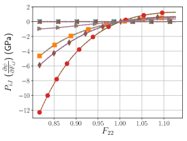
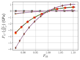
(a)	(b)	(c)
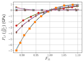
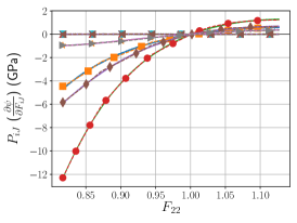
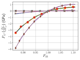
(d)	(e)	(f)

Figure 11: Comparison of the predicted stress response against three uniaxial MD simulations for the energy conjugate pair $\boldsymbol{P}-\boldsymbol{F}$ models $\mathcal{M}_{2}$ and $\mathcal{M}_{4}$. (a,d) Uniaxial compression and extension along the $x_{1}$ axis for models $\mathcal{M}_{2}$ and $\mathcal{M}_{4}$ respectively. (b,e) Uniaxial compression and extension along the $x_{2}$ axis for models $\mathcal{M}_{2}$ and $\mathcal{M}_{4}$ respectively. (c,f) Uniaxial compression and extension along the $x_{3}$ axis for models $\mathcal{M}_{2}$ and $\mathcal{M}_{4}$ respectively.

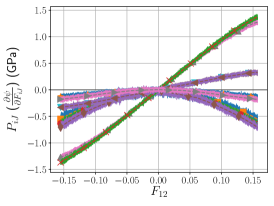
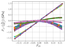
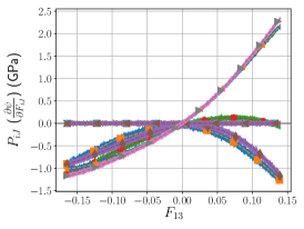
(a)	(b)	(c)

Figure 12: Comparison of the predicted 1st Piola-Kirchhoff stress response against three shear MD simulations for the energy conjugate pair $\boldsymbol{P}-\boldsymbol{F}$ model ($\mathcal{M}_{2}$). (a) Shear tests along the asymmetric positive and negative $\boldsymbol{e}_{1}\otimes\boldsymbol{e}_{2}$ direction. (b) Shear tests along the asymmetric positive and negative $\boldsymbol{e}_{2}\otimes\boldsymbol{e}_{3}$ direction. (c) Shear tests for the asymmetric positive and negative $\boldsymbol{e}_{1}\otimes\boldsymbol{e}_{3}$ direction.

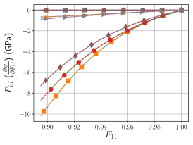
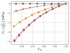
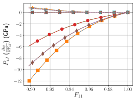
(a)	(b)	(c)

Figure 13: Comparison of the predicted 1st Piola-Kirchhoff stress response against three biaxial MD simulations for the energy conjugate pair $\boldsymbol{P}-\boldsymbol{F}$ model ($\mathcal{M}_{2}$). (a) Biaxial compression along the $x_{1}$ and $x_{2}$ axes. (b) Biaxial compression along the $x_{2}$ and $x_{3}$ axes. (c) Biaxial compression along the $x_{1}$ and $x_{3}$ axes.