Spectral reconstruction in NRQCD via the Backus-Gilbert method

Abstract

We present progress results from the Fastsum collaboration’s programme to determine the spectrum of the bottomonium system as a function of temperature using a variety of approaches. In this contribution, the Backus-Gilbert method is used to reconstruct spectral functions from NRQCD meson correlator data from Fastsum’s anisotropic ensembles at nonzero temperature. We focus in particular on the resolving power of the method, providing a demonstration of how the underlying resolution functions can be probed by exploiting the Laplacian nature of the NRQCD kernel. We conclude with estimates of the bottomonium ground state mass and widths at nonzero temperature.

1 Introduction

Bottomonium states play a special role in QCD at high temperature. They are produced copiously in current relativistic heavy-ion collision experiments and can act as probes of the quark-gluon plasma, as their masses are much larger than other energy scales, including the temperature.

Spectral studies of bottomonium systems at nonzero temperature using lattice QCD are challenging due to the “ill-posed” nature of spectral reconstruction. The Fastsum Collaboration has studied bottomonium using lattice QCD at nonzero temperature on anisotropic lattices for some time [1, 2, 3]. Here we discuss attempts to study the bottomonium spectrum using our thermal, anisotropic lattices using a variety of different methods. In this contribution the Backus-Gilbert method is used; in other contributions the Maximum Likelihood [4] and Kernel Ridge Regression [5] are applied.

2 Lattice details

The large mass of the $b$ quark means that $M_{b}\gg T$ and so the nonrelativistic QCD (NRQCD) effective field theory can be used to study bottomonium mesons. In this approximation, the Lagrangian is expanded in powers of the $b$ quark velocity, where expansions up to $\mathcal{O}(v^{4})$ are sufficient to describe the behaviour of the $b$ [6]. Because the $b$-quark and antiquark decouple, the time evolution of the $b$-quark propagator becomes an initial-value problem.

In NRQCD, the spectral representation of the Euclidean meson correlator, $G(\tau)$, is given by

$$G(\tau;T)=\int_{\omega_{\text{min}}}^{\omega_{\text{max}}}\frac{d\omega}{2\pi}K(\tau,\omega)\rho(\omega;T)$$ (1)

where $\rho(\omega;T)$ is the spectral density at temperature $T=(a_{\tau}N_{\tau})^{-1}$ as a function of the energy $\omega$ and $K(\tau,\omega)$ is the temperature independent kernel of NRQCD, $K(\tau,\omega)=e^{-\omega\tau}$. We note that there is an additive energy rescaling inherent in NRQCD, and so the $\omega$ energy range is related to the physical energy via

$$E^{\text{physical}}=\omega+\Delta E,\qquad\qquad\Delta E=7.46\,\text{GeV}.$$ (2)

This analysis makes use of Fastsum’s Generation 2L ensembles: anisotropic lattices ($\xi=a_{s}/a_{\tau}\sim 3.5$) with 2+1 flavour, clover-improved Wilson fermions using a physical $s$ quark and lighter, degenerate $u$ and $d$ quarks (see [7] for details). The spatial extent of the lattice $N_{s}=32$ and there are $\mathcal{O}(1000)$ configurations at each temperature. Details of the temperatures studied and the corresponding temporal extent, $N_{\tau}$, are listed in Table 1.

$N_{\tau}$	128	64	56	48	40	36	32	28	24	20	16
$T=1/(a_{\tau}N_{\tau})$ [MeV]	47	94	107	125	150	167	187	214	250	300	375

Table 1: Temporal extent and temperature in MeV for the Fastsum Generation 2L ensembles [7].

3 The Backus-Gilbert method

To solve Eq. (1) for $\rho(\omega)$, we first note that $G(\tau)$ is usually known at only $\mathcal{O}(10)-\mathcal{O}(100)$ points, whereas it would require $\mathcal{O}(1000)$ points to correctly represent the continuous function $\rho(\omega)$. This illustrates the “ill-posed” nature of this inverse problem.

Backus and Gilbert introduced their method for solving this problem in the context of inverting gross Earth data in 1968 [8]. Their method’s estimate, $\hat{\rho}$, of the solution to Eq. (1) is generated from the target spectrum $\rho$ via a set of resolution functions $A(\omega,\omega_{0})$,

$$\hat{\rho}(\omega_{0})=\int_{\omega_{\text{min}}}^{\omega_{\text{max}}}A(\omega,\omega_{0})\rho(\omega)d\omega.$$ (3)

Ideally $A(\omega,\omega_{0})$ closely approximates the delta function $\delta(\omega-\omega_{0})$. The key point is that the resolution functions are a linear combination of the kernel,

$$A(\omega,\omega_{0})=\sum_{\tau}c_{\tau}(\omega_{0})K(\tau,\omega).$$ (4)

where $c_{\tau}(\omega_{0})$ are the yet-to-be-determined Backus-Gilbert coefficients. Combining Eqs. (3) and (4), the spectrum estimate $\hat{\rho}$ can now be expressed linearly in terms of the correlation function,

$$\hat{\rho}(\omega_{0})=\sum_{\tau}c_{\tau}(\omega_{0})G(\tau).$$ (5)

We use the “least-squares” or “Dirichlet” approach to determine the coefficients $c_{\tau}(\omega_{0})$. This minimises the distance $J$ between the resolution functions and the delta function [9],

$$J(\omega_{0})=\int_{\omega_{\text{min}}}^{\omega_{\text{max}}}\left[A(\omega,\omega_{0})-\delta(\omega-\omega_{0})\right]^{2}~{}d\omega.$$ (6)

The coefficients $c_{\tau}(\omega_{0})$ corresponding to the minimisation of Eq. (6) can be found by solving the matrix-vector product,

$$\mathcal{K}_{\tau\tau^{\prime}}\cdot c_{\tau^{\prime}}(\omega_{0})=K(\omega_{0},\tau),\qquad\text{where}\quad\mathcal{K}_{\tau\tau^{\prime}}=\int_{\omega_{\text{min}}}^{\omega_{\text{max}}}K(\tau,\omega)K(\tau^{\prime},\omega)d\omega.$$ (7)

The kernel width matrix $\mathcal{K}$ is almost singular and it is therefore necessary to impose a regularisation routine in order to invert Eq. (7). This is achieved by adding the covariance matrix $\Sigma$ of the underlying data, $G(\tau)$, to $\mathcal{K}$ [10],

$$\mathcal{K}(\alpha)=\alpha\mathcal{K}+(1-\alpha)\Sigma,$$ (8)

where $\alpha\in(0,1]$ is the parameter which determines the strength of the regularisation.

A consequence of this redefinition is that there is a counter-play between the resolution width, i.e. the ability of the method to resolve fine spectral features, and the stability of the solution [11, 12]; the greater the regularisation, the worse the method’s resolving power.

4 Results for the $\Upsilon$ meson

We use NRQCD correlation functions computed on Fastsum’s anisotropic ensembles [7] to estimate the $\Upsilon$ ground state mass, $M$, and width, $\sigma$ using the Backus-Gilbert method outlined above. In Fig.1 we present results for the Backus-Gilbert $\Upsilon$ spectral function $\hat{\rho}$ at four temperatures. In these plots, $\alpha=0.1$ (see Eq. (8)) and $\omega_{\text{min}}=8.66$ GeV. The vertical magenta dashed line shows the experimental value of the $\Upsilon$ mass. As can be seen, the Backus-Gilbert estimate changes less as the temperature decreases, even though the number of $\tau$-points, and therefore the efficacy of the method increases as $T\rightarrow 0$.

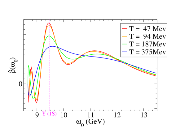
Figure 1: $\Upsilon$ spectrum as predicted by the Backus-Gilbert method at four temperatures for the choice $\omega_{\text{min}}\approx 8.66$ GeV and $\alpha=0.1$. Local quark sources were used. The magenta line is the experimental value of the $\Upsilon$ mass [13]. The statistical error in $\hat{\rho}(\omega_{0})$, estimated via bootstrap resampling, is too small to be seen.

The explicit dependence of $\hat{\rho}(\omega_{0})$ on $\alpha$ and $\omega_{\text{min}}$ is unknown. We therefore estimate this systematic error from an ensemble of $\mathcal{O}(500)$ choices of $\alpha$ and $\omega_{\text{min}}$, with $\alpha$ ranging from 1.0 (no regularization) to $10^{-5}$ and $\omega_{\text{min}}$ ranging from $-0.2a_{\tau}^{-1}$ to $0.2a_{\tau}^{-1}$ (which in physical units is $\approx 6.26$ GeV to $\approx 8.66$ GeV, see Eq. (2)). In addition, a bootstrap analysis using 1000 samples drawn from the Monte Carlo ensemble of $G(\tau)$ is used to determine the statistical error. The largest contribution to the error in $\hat{\rho}(\omega_{0})$ is from systematic sources (see Fig. 3). Fig. 1 shows that the statistical error in $\hat{\rho}(\omega_{0}$) estimated by using samples $G(\tau)$ is small, although these errors do become significant in the case of either Laplace shifting (see Fig. 4) or when there is little to no regularisation, see Eq. (8).

The ground state feature is found by seeking the peak nearest to the expected mass $\approx 9.4$ GeV. The ground state mass $M$ and width $\sigma$ are then extracted via a Gaussian fit to the top 50% of the leading edge (i.e. $\omega\leq M$) of this peak. The trailing edges (i.e. $\omega\geq M$) are not included in these Gaussian fits because they tend to be contaminated by contributions from higher energy states. There are often “side-lobe” artefact features below this ground state. To ensure only robust estimates are included in the analysis, cases where these artefacts reach more than 50% of the ground state’s peak are discarded.

The number of rejected fits increases as $T\rightarrow 0$ due to small-$\omega$ oscillations in the construction of the $A(\omega,\omega_{0})$. For temperatures $T>50$ MeV ($N_{\tau}<128$), the routine rejects $<10$% of fits. For the lowest temperature of $T\simeq 47$ MeV ($N_{\tau}=128$), results from around 80% of the tested parameter pairs were rejected.

Fig. 2 shows estimates for the ground state mass and width using this procedure as a function of temperature. Both local and smeared quark sources are used where the smearing was chosen to have a good overlap with the ground state. The ground state width appears independent of source type for all $T$ considered. In the case of the ground state mass, the approach to the $T=0$ estimate differs between source types. Given this difference in behaviour, it is uncertain whether the ground state mass increases or decreases with increasing temperature.

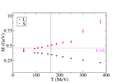
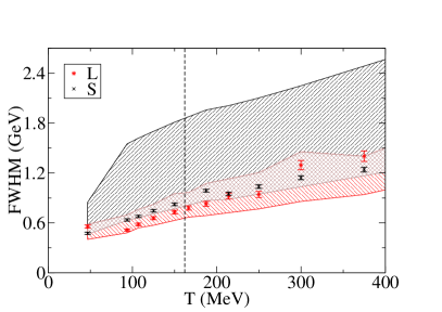
Figure 2: Ground state mass $M$ (left) and full width at half maximum (FWHM, right) versus temperature in the $\Upsilon$ channel with local (L) and smeared (S) sources. The horizontal magenta line is the experimental value for the $\Upsilon$ mass and the vertical black line is the pseudo-critical temperature, $T_{\rm pc}=162(1)$ MeV, determined by the inflection point of the renormalised chiral condensate [7]. The shaded regions indicate the minimum resolvable width for local (red) and smeared (black) sources, see below.

5 Systematic errors and improvements

Varying the Euclidean time window – At small $\tau$, $G(\tau)$ sees contributions from excited states. One could imagine restricting the time window, $[\tau_{1},\tau_{2}]$, to include large Euclidean times only where these excited states are exponentially suppressed. However, restricting the $[\tau_{1},\tau_{2}]$ interval reduces the number of kernel functions used to construct the resolution function $A(\omega,\omega_{0})$ which consequentially limits the resolving power of the method. For this reason, our analysis includes the full time range, $[\tau_{1},\tau_{2}]=[0,N_{\tau}-1]$.

Varying $\omega_{\text{min}}$ and $\alpha$ – As discussed in Sec. 4, we generate Backus-Gilbert estimates at multiple values of $\alpha$ and $\omega_{\text{min}}$ to probe the systematics related to these two quantities. We note that the resolving power of the Backus-Gilbert approach depends on both $\omega_{\text{min}}$ and $\alpha$. It is a feature of the Backus-Gilbert approach that its resolution is best for features nearest $\omega_{\text{min}}$, and therefore the resolution improves as $\omega_{\text{min}}$ increases. Also, as discussed in Sec. 3, the resolution increases with $\alpha$. These two features are illustrated in Fig. 3 where the mass and full width at half maximum (FWHM) are plotted against $\omega_{\text{min}}$. Different values of $\alpha$ are shown using the colour coding indicated. As can be seen the FWHM decreases (i.e. the resolution increases) with $\omega_{\text{min}}$. The same is observed as $\alpha$ increases, for fixed $\omega_{\text{min}}$.

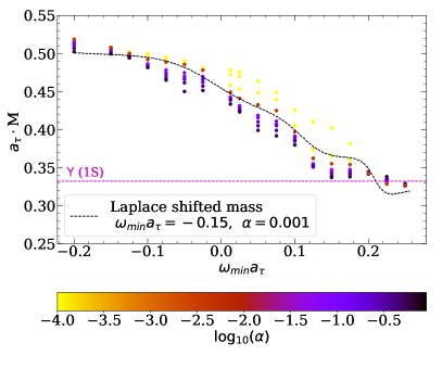
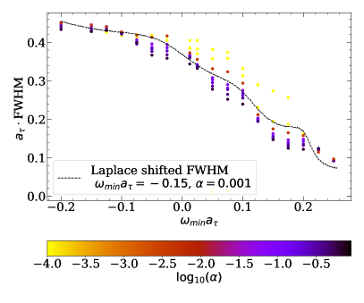
Figure 3: Scatter plot showing how the mass $M$ (left) and FWHM (right) of the ground state changes with $\omega_{\text{min}}$ and $\alpha$, indicating the systematic improvement in resolution. The horizontal magenta line is the experimental estimate of the $\Upsilon$ mass and $T=375$ MeV. In addition, in the case of Laplace shifts, the dashed line shows how $M$ and FWHM change with $\Delta$ for the case of $\omega_{\text{min}}a_{\tau}=-0.15$ and $\alpha=0.001$. Note that the Laplace shifted $M$ and FWHM are plotted against $-0.15+\Delta$ so that a direct comparison can be made with the $\omega_{\text{min}}$-varying case. This indicates a Laplace shift is equivalent to changing the lower bound $\omega_{\text{min}}$.

Laplace shifting and noise subtraction – The exponential nature of the NRQCD kernel means that the spectral representation of the Euclidean correlator in Eq. (1) is functionally identical to the Laplace transform. Of particular interest is the frequency shifting rule:

$$G^{\prime}(\tau)=e^{\Delta\cdot\tau}G(\tau)\overset{\mathcal{L}}{\Longrightarrow}\rho^{\prime}(\omega)=\rho(\omega+\Delta),$$ (9)

where $\Delta$ is the shift parameter and $\rho(\omega)$ is the Laplace transform of $G(\tau)$. However, the Backus-Gilbert spectral function, $\hat{\rho}(\omega_{0})$, will only be the true Laplace transform of $G(\tau)$ in the limit that $A(\omega,\omega_{0})=\delta(\omega-\omega_{0})$, see Eq. (3), which is not achievable on a finite system. We also note that the averaging functions $A(\omega,\omega_{0})$ are invariant under the shift. This means that because the shifted spectrum’s ground state features are closer to $\omega_{\text{min}}$, it will have better resolution. In this way, the Laplace shift should play a similar role to the $\omega_{\text{min}}$ shift. This is tested and confirmed in Fig. 3 where the Laplace shifted spectrum’s mass and FWHM is shown by the dashed curve. This nicely overlays the results obtained from the $\omega_{\text{min}}$ shift.

In Fig. 4 (left) the Laplace-shifted spectral functions are plotted for a variety of $\Delta$. The enhanced resolution of the ground state feature as $\Delta$ increases can clearly be seen. However, this comes at the expense of larger unphysical features in the small-$\omega$ region. This behaviour can be suppressed via an empirical noise subtraction procedure. The expression

$$\bar{A}(\omega_{0})=\int_{\omega_{\text{min}}}^{\omega_{\text{max}}}A(\omega,\omega_{0})~{}d\omega$$ (10)

is the Backus-Gilbert prediction for a flat spectrum, $\rho(\omega)=\text{constant}$. It is observed to closely match the unphysical small-$\omega$ fluctuations. We use this to define the noise-subtracted spectral function,

$$\hat{\rho}^{\text{subtracted}}(\omega_{0})=\hat{\rho}(\omega_{0})-\gamma\bar{A}(\omega_{0}),$$ (11)

where $\gamma$ is tuned to minimise the small-$\omega$ fluctuations. Fig. 4 (right) plots $\hat{\rho}^{\text{subtracted}}$ which shows a reduction in the unphysical features below the ground state confirming the usefulness of this noise subtraction procedure.

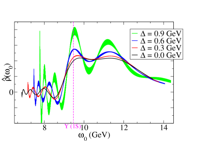
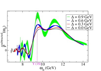
Figure 4: Left: Backus-Gilbert spectral functions at $T=187$ MeV for a variety of Laplace shifts, $\Delta$, showing enhanced resolution as $\Delta$ increases. The magenta line is the experimental value of the $\Upsilon$ mass [13]. Right: The same spectral functions, but this time with noise subtraction using Eq. (11). This shows a reduction in the unphysical features in the energy range below the ground state.

Assessment of the resolving power – From Eq. (3), the resolution function, $\hat{\rho}(\omega_{0})=A(M,\omega_{0})$, is the Backus-Gilbert prediction for the case of a spectral function $\rho(\omega)=\delta(\omega-M)$. It therefore gives us a measure of the narrowest feature that the method can resolve.

We determine the FWHM of $A(M,\omega_{0})$, using the same fit and rejection criteria as outlined in Sec. 4. Fig. 2 (Right) depicts these resolution FWHM values for the range of $T$ considered for both the local and smeared cases. These are a band of values because there is an ensemble of $\omega_{\text{min}}$ and $\alpha$ values included, see Sec. 4. Since the Backus-Gilbert results do not sit above these resolution band, we conclude that the method is unable to resolve the width of the ground state.

We explore these issues further by applying the Backus-Gilbert method to a test spectrum consisting of a single, broad Gaussian of width $\sigma\simeq 1.4$ GeV centred at $M_{\Upsilon}\sim 9.4$ GeV. The same $N_{\tau}$ range as in Table 1 was used, with the same coefficient set, $c_{\tau}(\omega_{0})$ as the local $\Upsilon$ data. The results of the Backus-Gilbert FWHM are shown in Fig. 5 together with the resolution band. As can be seen, the width estimate exceeds the resolution for $T\lesssim 300$ MeV. This behaviour is what one would ought to expect if the method was indeed capable of resolving the feature width and contrasts with the results we find in Fig. 2. It is for this reason that we believe our estimates of the ground state width instead represent an upper bound only.

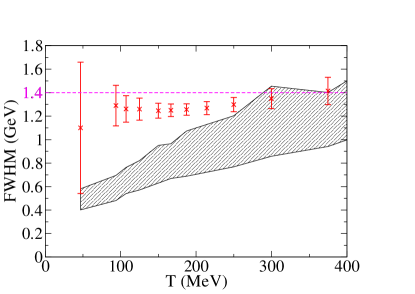
Figure 5: Plot of the FWHM obtained from the Backus-Gilbert method applied to a test spectrum of width $\sigma\simeq 1.4$ GeV. The same values of $N_{\tau}$ were used as in Table 1. Note that the large error bar for the smallest temperature is due to a high number of rejected fits (see Sec. 4). The grey region represents the resolution band.

6 Summary

We have presented preliminary results for the ground state mass and width for the $\Upsilon$ meson, using both local and smeared quark sources. Since the widths are found to be consistent with the minimum resolvable width from the method, we consider our estimates of the ground state width to be upper bounds only.

We have also shown how the Laplace frequency shift transform or a shift of the energy window may be used to improve the resolving power of the method, with the caveat that a noise reduction routine must be employed to control unphysical oscillations in the small energy region in the former case.

References

- [1] G. Aarts, S. Kim, M.P. Lombardo, M.B. Oktay, S.M. Ryan, D.K. Sinclair et al., Bottomonium above deconfinement in lattice nonrelativistic QCD, Phys. Rev. Lett. 106 (2011) 061602 [1010.3725].
- [2] G. Aarts, C. Allton, S. Kim, M.P. Lombardo, M.B. Oktay, S.M. Ryan et al., What happens to the and in the quark-gluon plasma? Bottomonium spectral functions from lattice QCD, JHEP 11 (2011) 103 [1109.4496].
- [3] G. Aarts, C. Allton, T. Harris, S. Kim, M.P. Lombardo, S.M. Ryan et al., The bottomonium spectrum at finite temperature from Nf = 2 + 1 lattice QCD, JHEP 07 (2014) 097 [1402.6210].
- [4] T. Spriggs et al., PoS LATTICE2021 (2021) 077.
- [5] S. Offler et al., PoS LATTICE2021 (2021) 509.
- [6] G.P. Lepage, L. Magnea, C. Nakhleh, U. Magnea and K. Hornbostel, Improved nonrelativistic QCD for heavy-quark physics, Physical Review D 46 (1992) 4052 [9205007].
- [7] G. Aarts, C. Allton, J. Glesaaen, S. Hands, B. Jäger, S. Kim et al., Properties of the QCD thermal transition with flavours of Wilson quark, 2007.04188.
- [8] G. Backus and F. Gilbert, The Resolving Power of Gross Earth Data, Geophysical Journal of the Royal Astronomical Society 16 (1968) 169.
- [9] D.W. Oldenburg, An Introduction to Linear Inverse Theory, IEEE Transactions on Geoscience and Remote Sensing GE-22 (1984) .
- [10] B.B. Brandt, A. Francis, H.B. Meyer and D. Robaina, Pion quasiparticle in the low-temperature phase of QCD, Physical Review D - Particles, Fields, Gravitation and Cosmology 92 (2015) 1 [1506.05732].
- [11] T.B. Yanovskaya, Inverse Problems of Geophysics, Tech. Rep. (IC–2003/54), International Atomic Energy Agency (IAEA) (2003), DOI.
- [12] B.J. Conrath, Backus-Gilbert Theory and its Application to Retrieval of Ozone Temperature Profiles, Tech. Rep. Goddard Space Flight Center (1977).
- [13] Particle Data Group, P.A. Zyla, R.M. Barnett, J. Beringer, O. Dahl, D.A. Dwyer et al., Review of Particle Physics, Progress of Theoretical and Experimental Physics 2020 (2020) .