Grass(mannian) trees and forests: Variations of the exponential formula, with applications to the momentum amplituhedron

Abstract.

The Exponential Formula allows one to enumerate any class of combinatorial objects built by choosing a set of connected components and placing a structure on each connected component which depends only on its size. There are multiple variants of this result, including Speicher’s result for noncrossing partitions, as well as analogues of the Exponential Formula for series-reduced planar trees and forests. In this paper we use these formulae to give generating functions for contracted Grassmannian trees and forests, certain graphs whose vertices are decorated with a helicity. Along the way we enumerate bipartite planar trees and forests, and we apply our results to enumerate various families of permutations: for example, bipartite planar trees are in bijection with separable permutations.

It is postulated by Livia Ferro, Tomasz Łukowski and Robert Moerman (2020) that contracted Grassmannian forests are in bijection with boundary strata of the momentum amplituhedron, an object encoding the tree-level S-matrix of maximally supersymmetric Yang-Mills theory. With this assumption, our results give a rank generating function for the boundary strata of the momentum amplituhedron, and imply that the Euler characteristic of the momentum amplituhedron is $1$.

1. Introduction

In recent years, scattering amplitudes research has motivated the study of amplituhedra, which can be viewed as generalizations of polytopes into Grassmannians. There are two amplituhedra relevant to the physics of tree-level particle scattering in maximally supersymmetric Yang-Mills theory: the (tree) amplituhedron $\mathcal{A}_{n,k,m}$, introduced by Arkani-Hamed–Trnka in [AHT14], and the momentum amplituhedron $\mathcal{M}_{n,k,m}$, introduced for $m=4$ by Damgaard–Ferro–Łukowski–Parisi in [DFŁP19] and later generalized to any even $m$ by Łukowski–Parisi–Williams in [ŁPW20]. For $m=4$, both the amplituhedron and the momentum amplituhedron encode tree-level scattering amplitudes in this theory, but using different kinematic spaces: the amplituhedron uses momentum twistor space while the momentum amplituhedron uses momentum space. Both objects are defined as the image of the totally nonnegative Grassmannian $\operatorname{Gr}_{k,n}^{\geq 0}$ under a particular map, where $\operatorname{Gr}_{k,n}^{\geq 0}$ is the subset of the real Grassmannian where all Plücker coordinates are nonnegative, first studied by Postnikov and Lusztig [Pos06, Lus94].

In addition to their physical significance when $m=4$, these amplituhedra are mathematically interesting objects which have been studied in various examples. For $k+m=n$, the amplituhedron is isomorphic to the totally nonnegative Grassmannian, whose rank generating function was computed in [Wil05]. When $k=1$, the amplituhedron is a cyclic polytope [AHT14], and when $m=1$, the amplituhedron is homeomorphic to the bounded complex of a cyclic hyperplane arrangement [KW19], which also has an explicit rank generating function. When $m=2$, the amplituhedron’s boundary strata were classified and enumerated in [Łuk19]. Less is known about the momentum amplituhedron $\mathcal{M}_{n,k,m}$, but for $m=4$, a conjectural characterization of the boundary strata of $\mathcal{M}_{n,k,4}$ (also denoted by $\mathcal{M}_{n,k}$) was given in [FŁM20]. The authors computed the rank generating functions for $\mathcal{M}_{n,k}$ for some small values of $k$ and $n$, and found in those cases that the Euler characteristic was $1$.

The goal of this paper is to enumerate the boundary strata of the $m=4$ momentum amplituhedron $\mathcal{M}_{n,k}$ (for any $k$ and $n$) according to their dimension. To do so, we begin by reformulating the speculative description of boundary strata from [FŁM20] in terms of Grassmannian forests, which are acyclic Grassmannian graphs. (Grassmannian graphs first appeared implicitly in [AHBC⁺16] as a generalization of plabic graphs, and were subsequently studied in [Pos18].) Having described the boundary strata in terms of Grassmannian forests, we proceed to enumerate Grassmannian forests using two variations of the well-known Exponential Formula. The first is Speicher’s analogue of the Exponential Formula for non-crossing partitions [Spe94]. The second variation is an analogue for series-reduced planar trees; it can be viewed naturally in the theory of species, and can also be viewed as a combinatorial interpretation of Lagrange Inversion, see [BLL98, Ard15]. Putting together these two variations leads to an analogue of the Exponential Formula for series-reduced planar forests, which we use to enumerate contracted Grassmannian forests according to helicity and momentum amplituhedron dimension. Along the way, we also enumerate contracted plabic trees and forests, which are in bijection with bipartite planar trees and forests. And we can translate all of our results into enumerative results about various class of permutations: for example, contracted plabic trees are in bijection with separable permutations.

The paper is structured as follows. In Section 2, we review the Lagrange Inversion formula and Speicher’s noncrossing partition analogue of the Exponential Formula. We then give series-reduced planar tree and forest analogues of the Exponential Formula. In Section 3, we introduce the totally nonnegative Grassmannian, as well as Grassmannian graphs, trees, and forests. We enumerate contracted plabic trees and forests as a warmup, keeping track of their helicity $k$, number of boundary vertices $n$, and their momentum amplituhedron dimension. We then enumerate contracted Grassmannian trees and forests according to the same statistics. In Section 4 we give applications to enumeration of permutations. In Section 5 we define the momentum amplituhedron $\mathcal{M}_{n,k}$ and interpret our combinatorial results as enumerating the boundary strata of $\mathcal{M}_{n,k}$. By specializing $q=-1$ in our generating function, we also find that the Euler characteristic equals $1$. We emphasise that the results of Section 5 assume the characterization of momentum amplituhedron boundaries conjectured in [FŁM20]. We end the paper with an appendix providing a table of rank generating functions for the momentum amplituhedron $\mathcal{M}_{n,k}$ for various values of $n$ and $k$.

2. Variations of the Exponential Formula

Many combinatorial objects can be built by choosing a set of connected components, then placing some structure on each connected component. In this case, if one understands how to enumerate the ways of placing a structure on each connected component of a given size, then the well-known Exponential Formula (see e.g. [Sta99, BLL98, Ard15]) allows one to enumerate the combinatorial objects. There is an analogue of the Exponential Formula, due to Speicher [Spe94], for combinatorial objects which can be built by choosing a noncrossing partition and then placing a structure on each block of the noncrossing partition. In this section we will provide background on Lagrange Inversion and Speicher’s result, then give analogues of the Exponential Formula for series-reduced planar trees and forests.

2.1. Lagrange Inversion

The set $xK[[x]]$ of all formal power series $a_{1}x+a_{2}x^{2}+\dots$ with zero constant term over a field $K$ forms a monoid under the operation of functional composition. The identity element of this monoid is the power series $x$.

Definition 2.1.

If $f(x)=a_{1}x+a_{2}x^{2}+\dots\in K[[x]]$, then we call a power series $g(x)$ a compositional inverse of $f$ if $f(g(x))=g(f(x))=x$, in which case we write $g(x)=f^{\langle-1\rangle}(x)$.

Theorem 2.2 (Lagrange inversion formula, [Sta99, Theorem 5.4.2]).

Let $K$ be a field with $\text{char}\,K=0$, and let $C(x)\in xK[[x]]$ with $[x]C(x)\neq 0$. Then for positive integers $k,n$ we have

$$n[x^{n}]C^{\langle-1\rangle}(x)^{k}=k[x^{n-k}]\left(\frac{x}{C(x)}\right)^{n}.$$

2.2. Speicher’s noncrossing partition analogue of the Exponential Formula

Definition 2.3.

A noncrossing partition of $[n]$ is a partition $\pi$ of the set $[n]=\{1,2,\dots,n\}$ into blocks $B_{1},\dots,B_{\ell}$ satisfying the following condition: if $a<b<c<d$ and $B$ and $B^{\prime}$ are blocks of $\pi$ such that $a,c\in B$ and $b,d\in B^{\prime}$, then $B=B^{\prime}$.

Equivalently, $\pi$ is a noncrossing partition if after drawing the numbers $1,2,\dots,n$ in order around a circle, and replacing each block $B$ with the convex hull of the corresponding points, the resulting polygons do not overlap. See Figure 1.

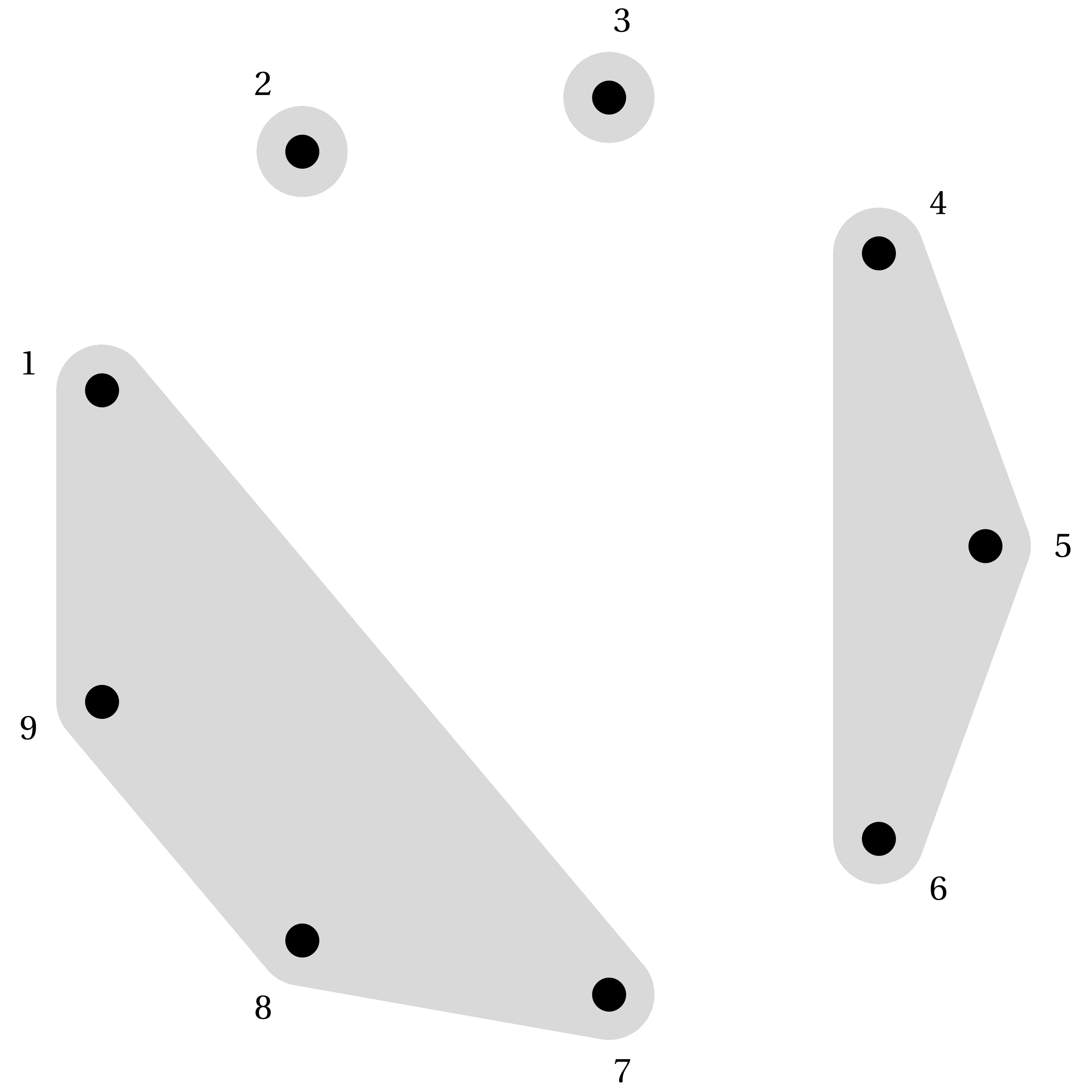
Figure 1. The non-crossing partition $\{\{1,7,8,9\},\{2\},\{3\},\{4,5,6\}\}$ of $[9]$ with each block drawn as a convex hull of the corresponding points.

Let $\operatorname{NC}_{n}$ denote the lattice of noncrossing partitions of $[n]$. The following result says that if a class $\mathcal{H}_{\operatorname{NC}}$ of combinatorial objects is built by choosing a noncrossing partition and putting a structure on each block independently (encoded by the function $f$), then the generating function $H_{\operatorname{NC}}(x)$ for $\mathcal{H}_{\operatorname{NC}}$ can be obtained from the generating function $F(x)$ for $f$.

Theorem 2.4 ([Spe94], see also [Sta99, Exercise 5.35b]).

Let $K$ be a field. Given a function $f:\mathbb{Z}^{+}\to K$, define a new function $h:\mathbb{Z}^{+}\to K$ by

$$h(n)=\sum_{\pi=\{B_{1},\dots,B_{\ell}\}\in\operatorname{NC}_{n}}f(\#B_{1})f(\#B_{2})\dots f(\#B_{\ell}),$$

where $\#B_{i}$ denotes the cardinality of block $B_{i}$. Let $F(x)=1+\sum_{n\geq 1}f(n)x^{n}$ and $H_{\operatorname{NC}}(x)=1+\sum_{n\geq 1}h(n)x^{n}$. Then

$$xH_{\operatorname{NC}}(x)={\left(\frac{x}{F(x)}\right)}^{\langle-1\rangle}.$$

2.3. Series-reduced planar tree and forest analogues of the Exponential Formula

In this section we give Theorem 2.9 and Corollary 2.13 which can be viewed as analogues of Speicher’s Theorem, but with series-reduced planar trees and planar forests replacing noncrossing partitions. We note that the result on series-reduced planar trees can be viewed as an analogue of Speicher’s Theorem for polygon dissections.

Definition 2.5.

A planar tree $T$ (respectively, a planar forest $F$) on $n$ leaves is a tree (resp., a forest) properly embedded in a disk with $n$ boundary vertices (i.e. vertices of degree $1$) on the boundary of the disk (labelled in clockwise order). Let $\operatorname{\mathcal{V}}_{\text{int}}(T)$ and $\operatorname{\mathcal{V}}_{\text{int}}(F)$ denote the set of internal vertices (i.e. vertices with degree at least $2$) of $T$ and $F$.

A planar tree or forest is called series-reduced if it has no internal vertices of degree $2$. Let $\mathcal{T}_{n}$ (resp., $\mathcal{F}_{n}$) denote the set of series-reduced planar trees (resp., forests) on $n$ leaves. (The requirement on internal vertices implies that $\mathcal{T}_{n}$ and $\mathcal{F}_{n}$ are finite.) A series-reduced planar tree $T$ on $n$ leaves is said to be of type $\bm{r}=(r_{3},\ldots,r_{n})$ if it has $r_{i}$ internal vertices of degree $i$. An example of a series-reduced planar tree on $9$ leaves of type $(2,1,1,0,0,0,0)$ is given in Figure 2 (middle). Let $\mathcal{T}_{n}(r_{3},\ldots,r_{n})$ denote the subset of $\mathcal{T}_{n}$ of type $(r_{3},\ldots,r_{n})$.

Definition 2.6.

A plane tree on $n-1$ leaves is a rooted tree $\tilde{T}$ with $n-1$ boundary vertices (i.e. vertices with no descendants) where each internal vertex of $\tilde{T}$ has at least $1$ descendant.

A Schröder tree is a plane tree which is series-reduced, i.e. each internal vertex has at least two descendants. A Schröder tree $\tilde{T}$ on $n-1$ leaves is said to be of type $(r_{3},\ldots,r_{n})$ if it has $r_{i}$ internal vertices with $i-1$ descendants. An example of a Schröder tree on $8$ leaves of type $(2,1,1,0,0,0,0)$ is given in Figure 2 (left). Let $\tilde{\mathcal{T}}_{n-1}$ denote the set of Schröder trees on $n-1$ leaves, and let $\tilde{\mathcal{T}}_{n-1}(r_{3},\ldots,r_{n})$ denote the subset of $\tilde{\mathcal{T}}_{n-1}$ of type $(r_{3},\ldots,r_{n})$.

Remark 2.7.

Given a series-reduced planar tree $T\in\mathcal{T}_{n}$, let $v_{\ast}$ be the internal vertex incident to the leaf labelled $1$. If we remove leaf $1$ and its incident edge, then the remaining tree $\tilde{T}$ can be thought of as a Schröder tree with root vertex $v_{\ast}$. This map gives a bijection between the series-reduced planar trees $T\in\mathcal{T}_{n}(r_{3},\ldots,r_{n})$ and Schröder trees $\tilde{T}\in\tilde{\mathcal{T}}_{n-1}(r_{3},\ldots,r_{n})$. Note that an internal vertex of degree $d$ in a series-reduced planar tree corresponds to an internal vertex with $d-1$ descendants in a Schröder tree.

Lemma 2.8.

Let $t_{n}(r_{3},\dots,r_{n})=|\mathcal{T}_{n}(r_{3},\ldots,r_{n})|$ be the number of series-reduced planar trees of type $\bm{r}=(r_{3},\ldots,r_{n})$ and let $|\bm{r}|=\sum_{i}r_{i}$. Then

$$t_{n}(r_{3},\ldots,r_{n})=\frac{(n+|\bm{r}|-2)!}{(n-1)!r_{3}!\cdots r_{n}!}.$$

Proof.

From Remark 2.7, series-reduced planar trees of type $(r_{3},\ldots,r_{n})$ are in bijection with the plane trees of type $(n-1,0,r_{3},\ldots,r_{n})$ considered in [Sta99, Section 5.3]. The formula in the lemma now follows from [Sta99, Theorem 5.3.10]. ∎

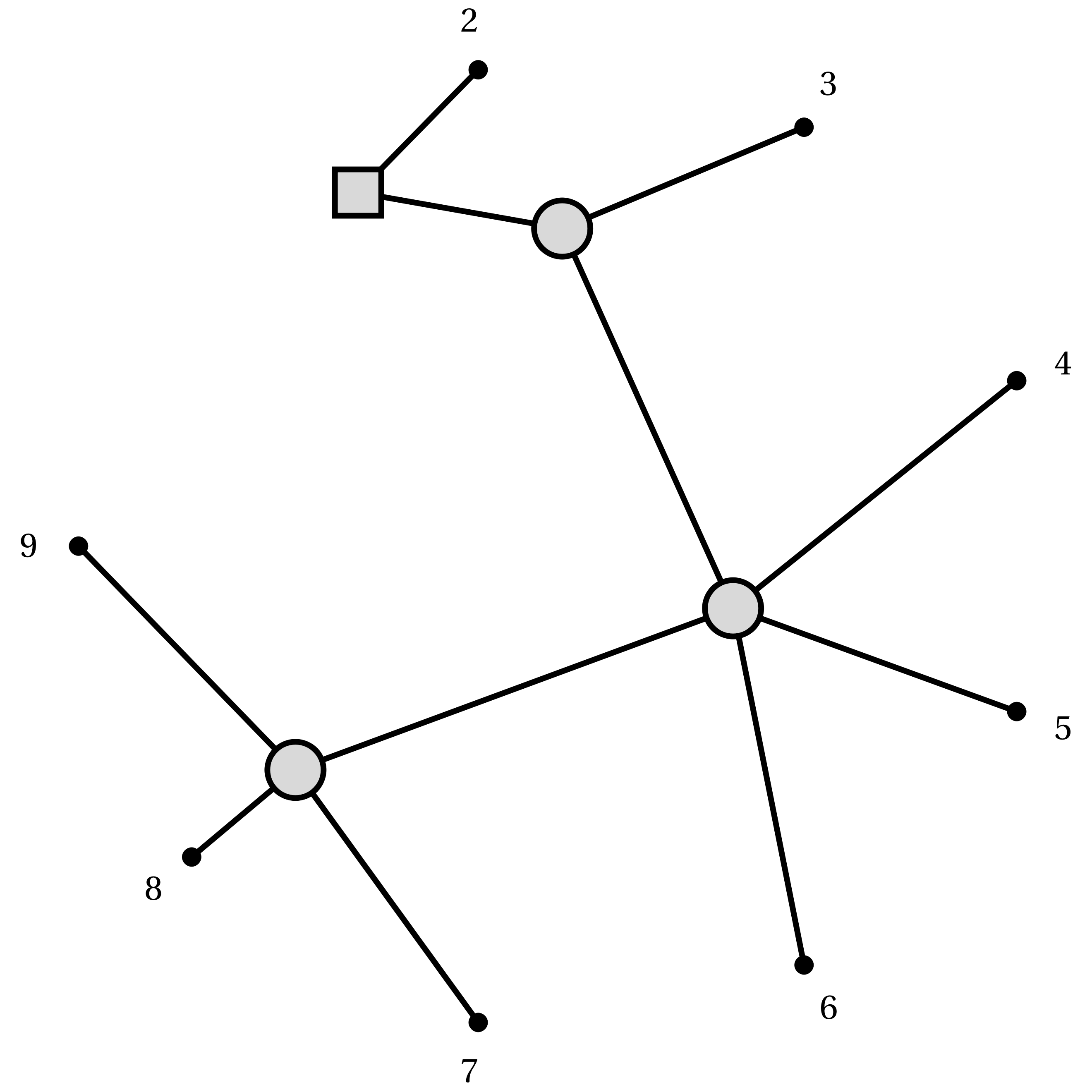
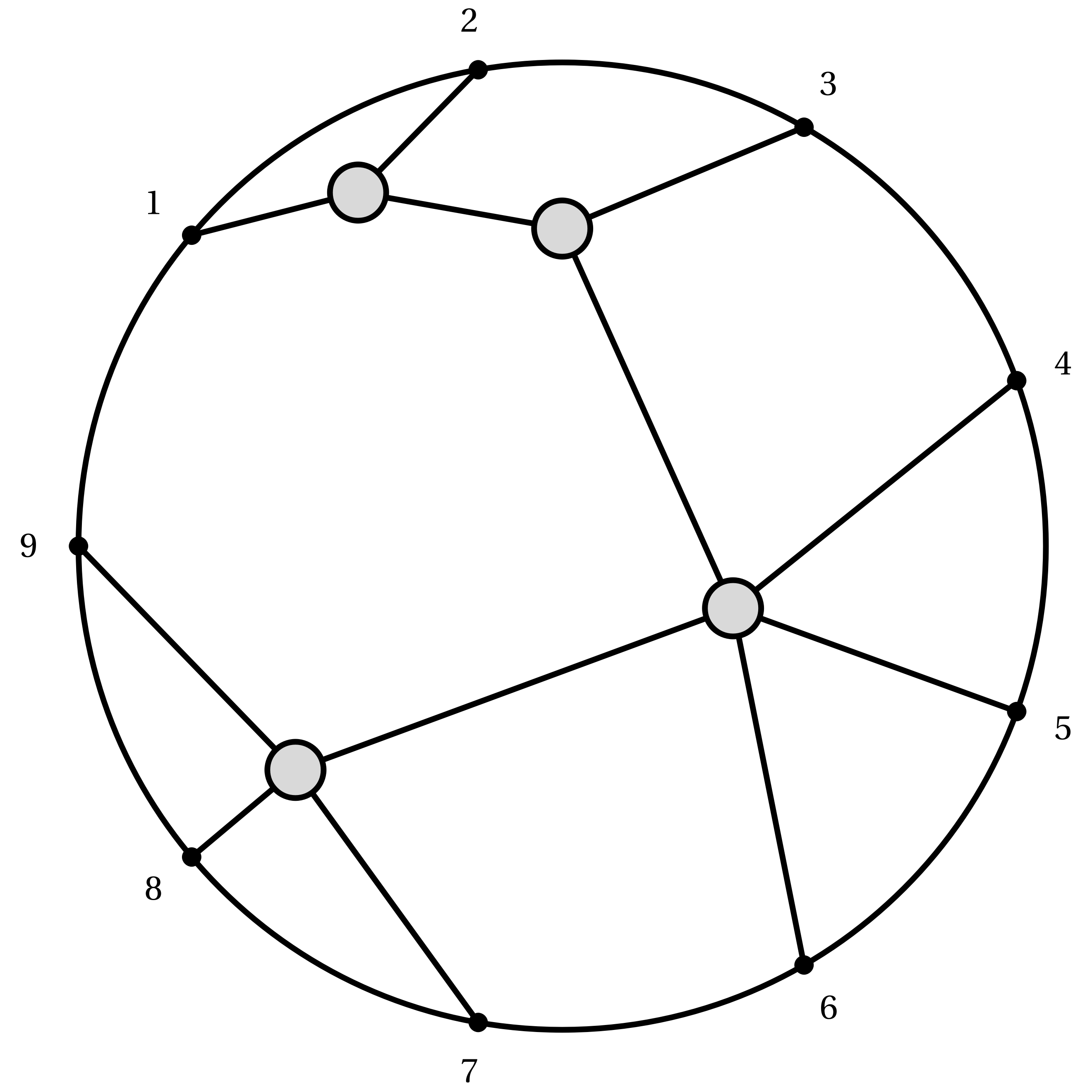
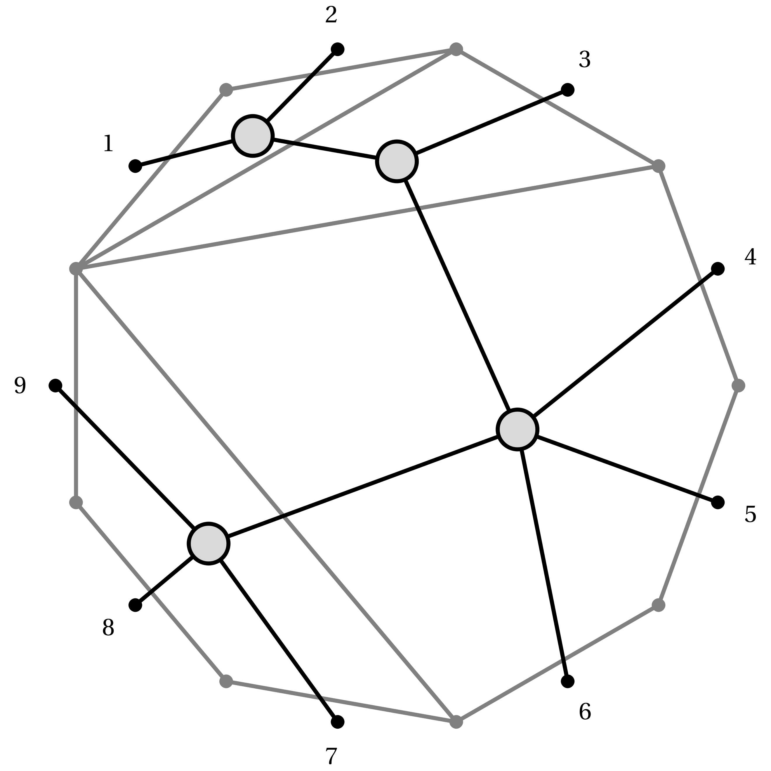
Figure 2. A series-reduced planar tree on $9$ leaves of type $(2,1,1,0,0,0,0,0)$ (middle), its corresponding Schröder tree on $8$ leaves with the root vertex depicted as a square (left), and its dual polygon dissection of $\mathbf{Q}_{9}$ (right).

The following result says that if a class $\mathcal{H}_{\operatorname{tree}}$ of combinatorial objects is built by choosing a series-reduced planar tree in $\mathcal{T}_{n}$ and putting a structure on each internal vertex independently (depending only on its degree and encoded by the function $f$), then the generating function $H_{\operatorname{tree}}(x)$ for $\mathcal{H}_{\operatorname{tree}}$ can be obtained from the generating function $F(x)$ for the function $f$. We note that Theorem 2.9 has appeared in various references: for example, it fits naturally into the theory of species and is closely related to [BLL98, page 168, Equation (18)]; it can also be reformulated using Schröder trees and viewed as a combinatorial interpretation of Lagrange Inversion, see [Ard15, Theorem 2.2.1]. It is similar in spirit to [JKM17, Proposition 5].

Theorem 2.9.

Let $K$ be a field. Given a function $f:\mathbb{Z}_{\geq 3}\to K$, define a new function $h:\mathbb{Z}_{\geq 3}\to K$ by

$$h(n)=\sum_{T\in\mathcal{T}_{n}}\prod_{v\in\operatorname{\mathcal{V}}_{\text{int}}(T)}f(\deg(v))\,.$$ (2.10)

Let $F(x)=\sum_{n\geq 3}f(n)x^{n}$ and $H_{\operatorname{tree}}(x)=x^{2}+\sum_{n\geq 3}h(n)x^{n}$. Then

$$\frac{1}{x}H_{\operatorname{tree}}(x)={\left(x-\frac{1}{x}F(x)\right)}^{\langle-1\rangle}.$$ (2.11)

Remark 2.12.

The appearance of the term $x^{2}$ in $H_{\operatorname{tree}}(x)$ reflects the fact that there is a unique series-reduced planar tree on $2$ leaves. If we want to account for the unique tree in $\mathcal{T}_{1}$ with $1$ leaf and $1$ internal vertex, we can consider $\hat{H}_{\operatorname{tree}}(x)=h(1)x+H_{\operatorname{tree}}(x)$, where $h(1)=f(1)$ is the number of structures that we can put on an internal vertex of degree $1$.

Theorem 2.9 can be proved in several ways.

1. Using Lemma 2.8, one can give an argument analogous to the proof of Speicher’s Theorem as presented in [Sta99, Exercise 5.35b]. We leave this as an exercise.

2. One can reformulate this result as a functional equation describing the recursive structure of trees. This can be verified directly but also fits naturally into Joyal’s framework of species as in [BLL98]. We thank Ira Gessel and Francois Bergeron for their comments on this approach; see also [Ard15, Theorem 2.2.1]). For completeness, we include this second proof below.

Proof of Theorem 2.9.

Let $\tilde{F}(x)=\frac{1}{x}F(x)=\sum_{n\geq 3}f(n)x^{n-1}$ and $\tilde{H}(x)=\frac{1}{x}H(x)=x+\sum_{n\geq 3}h(n)x^{n-1}$. That is, the coefficient of $x^{n-1}$ in $\tilde{F}(x)$ gives the number of ways of decorating an internal vertex $v$ in a Schröder tree where $v$ has $n-1$ descendants, and the coefficient of $x^{n-1}$ in $\tilde{H}(x)$ enumerates the decorated Schröder trees on $n-1$ leaves.

Schröder trees can be built by choosing a root vertex $v_{\ast}$ with degree $d-1$ (where $d\geq 3$) and placing Schröder trees $\tilde{T}_{1},\ldots,\tilde{T}_{d-1}$ at each of the $d-1$ vertices below $v_{\ast}$. Thus, it immediately follows that

$$\tilde{H}(x)=x+\sum_{n\geq 3}f(n)\tilde{H}(x)^{n-1}=x+\tilde{F}(\tilde{H}(x))\,,$$

which is equivalent to $\tilde{H}(x)=(x-\tilde{F}(x))^{\langle-1\rangle}$ or $\frac{1}{x}H(x)=(x-\frac{1}{x}F(x))^{\langle-1\rangle}$. ∎

We now combine Theorem 2.9 and Theorem 2.4 to obtain Corollary 2.13 below. As before, we interpret this result as saying that if a class $\mathcal{H}_{\operatorname{forest}}$ of combinatorial objects is built by choosing a series-reduced planar forest in $\mathcal{F}_{n}$ and putting a structure on each internal vertex independently (depending only on its degree and encoded by the function $g$), then the generating function $H_{\operatorname{forest}}(x)$ for $\mathcal{H}_{\operatorname{forest}}$ can be obtained from the generating function $G(x)$ for the function $g$.

Corollary 2.13.

Let $K$ be a field. Given a function $g:\mathbb{Z}^{+}\to K$, define a new function $h:\mathbb{Z}^{+}\to K$ by

$$h(n)=\sum_{F\in\mathcal{F}_{n}}\prod_{v\in\operatorname{\mathcal{V}}_{\text{int}}(F)}g(\deg(v)).$$ (2.14)

(Note that $h(1)=g(1)$, and that $g(2)$ is irrelevant for series-rooted forests.)

Let $G(x)=\sum_{n\geq 3}g(n)x^{n}$ and $H_{\operatorname{forest}}(x)=1+\sum_{n\geq 1}h(n)x^{n}$. Then

$$xH_{\operatorname{forest}}(x)={\left(\frac{x}{1+\hat{H}_{\operatorname{tree}}(x)}\right)}^{\langle-1\rangle}={\left(\frac{x}{1+h(1)x+x\left(x-\frac{G(x)}{x}\right)^{\langle-1\rangle}}\right)}^{\langle-1\rangle},$$ (2.15)

where $\hat{H}_{\operatorname{tree}}(x)$ is given by Remark 2.12 and (2.11).

Proof.

The connected components of a planar forest embedded in a disk have the structure of a noncrossing partition. So we can enumerate planar forests by applying Theorem 2.4, with $1+\hat{H}_{\operatorname{tree}}(x)$ playing the role of $F(x)$ (which has constant term $1$). The result now follows from Theorem 2.9. ∎

Although we don’t need it for what follows, we note that the trees in $\mathcal{T}_{n}$ are in bijection with dissections of a polygon.

Definition 2.16.

Let $\mathbf{Q}_{n}$ denote a convex $n$-gon with vertices labelled $1,2,\dots,n$. A dissection of $\mathbf{Q}_{n}$ is a subdivision $\rho$ of $\mathbf{Q}_{n}$ into smaller polygons $\{P_{1},\dots,P_{\ell}\}$ obtained by drawing diagonals that don’t intersect in their interiors. We say that a dissection of $\mathbf{Q}_{n}$ has type $(m_{3},\dots,m_{n})$ if it consists of $m_{i}$ $i$-gons. Figure 2 (right) gives an example of a dissection of $\mathbf{Q}_{9}$ of type $(2,1,1,0,0,0,0)$.

Clearly the series-reduced planar trees in $\mathcal{T}_{n}(m_{3},\dots,m_{n})$ are also in bijection with the dissections of $\mathbf{Q}_{n}$ of type $(m_{3},\dots,m_{n})$. Both of these objects are in bijection with the faces of the $(n-3)$-dimensional associahedron as well as its normal fan. The latter is combinatorially the Stanley–Pitman fan [SP02] or the tropical totally positive Grassmannian $\operatorname{Trop}^{+}\operatorname{Gr}_{2,n}$ [SW05].

We can now translate Theorem 2.9 into the language of polygon dissections. Let $\operatorname{D}_{n}$ denote the set of dissections of the $n$-gon $\mathbf{Q}_{n}$. The following theorem follows from the Implicit Species Theorem of Joyal [BLL98] and also appeared in [SW16, Theorem 4.2].

Theorem 2.17.

Let $K$ be a field. Given a function $f:\mathbb{Z}_{\geq 3}\to K$, define a new function $h:\mathbb{Z}_{\geq 3}\to K$ by

$$h(n)=\sum_{\rho=\{P_{1},\dots,P_{\ell}\}\in\operatorname{D}_{n}}f(\#P_{1})f(\#P_{2})\dots f(\#P_{\ell}),$$

where $\#P_{i}$ denotes the number of vertices in the polygon $P_{i}$. Let $F(x)=\sum_{n\geq 3}f(n)x^{n}$ and $H(x)=x^{2}+\sum_{n\geq 3}h(n)x^{n}$. Then

$$\frac{1}{x}H(x)={\left(x-\frac{1}{x}F(x)\right)}^{\langle-1\rangle}.$$

3. Grassmannian graphs, trees and forests

The totally nonnegative Grassmannian, a particular semi-algebraic subset of the real Grassmannian, was first introduced by Postnikov and Lusztig [Pos06, Lus94], and it has been a topic of intense investigation by both mathematicians and physicists. In this section we introduce the totally nonnegative Grassmannian together with (equivalence classes of) Grassmannian graphs, which index its cells. We also introduce Grassmannian forests, which (conjecturally) enumerate the boundary strata of a related object called the momentum amplituhedron. We then provide explicit enumeration formulae for Grassmannian trees and forests.

3.1. The totally nonnegative Grassmannian and its positroid stratification

Fix integers $k,n$ such that $0\leq k\leq n$. The Grassmannian $\operatorname{Gr}_{k,n}(\mathbb{F})$ over a field $\mathbb{F}$ is the variety of all $k$-dimensional subspaces of $\mathbb{F}^{n}$. Each element of $\operatorname{Gr}_{k,n}(\mathbb{F})$ may be represented by a full rank $k\times n$ matrix, modulo row operations, whose rows span the $k$-dimensional subspace. We denote the element of $\operatorname{Gr}_{k,n}(\mathbb{F})$ represented by the matrix $C$ by $[C]$.

In what follows, let $\operatorname{Gr}_{k,n}=\operatorname{Gr}_{k,n}(\mathbb{R})$ denote the real Grassmannian. Recall that $[n]:=\{1,2,\ldots,n\}$. Let $\binom{[n]}{k}$ denote the set of all $k$-element subsets of $[n]$. Given an element $V=[C]\in\operatorname{Gr}_{k,n}$, the maximal minors $\Delta_{I}(C)$ of $C$, where $I\in\binom{[n]}{k}$, form projective coordinates on $\operatorname{Gr}_{k,n}$, called the Plücker coordinates of $V$. Consequently, we write $\Delta_{I}(V)$ to denote $\Delta_{I}(C)$.

Definition 3.1 ([Pos06, Section 3]).

An element of $\operatorname{Gr}_{k,n}$ is said to be totally positive (resp., totally nonnegative) if all of its Plücker coordinates are positive (resp., nonnegative). The totally positive Grassmannian $\operatorname{Gr}_{k,n}^{>0}$ (resp., totally nonnegative Grassmannian $\operatorname{Gr}_{k,n}^{\geq 0}$) is the semi-algebraic subset of all totally positive (resp., totally nonnegative) elements of $\operatorname{Gr}_{k,n}$. For each $M\subset\binom{[n]}{k}$, let $S_{M}$ be the subset of elements of $\operatorname{Gr}_{k,n}^{\geq 0}$ whose Plücker coordinates are all strictly positive for $I\in M$ and otherwise zero. If $S_{M}$ is non-empty, $M$ is called a positroid and $S_{M}$ its positroid cell.

Each positroid cell is indeed a topological cell [Pos06, Theorem 6.5], and moreover, the positroid cells of $\operatorname{Gr}_{k,n}^{\geq 0}$ glue together to form a CW complex [PSW09].

It was shown in [Pos06] that positroid cells of $\operatorname{Gr}_{k,n}$ are in bijection with various combinatorial objects including (equivalence classes of) reduced plabic graphs $G$ of type $(k,n)$, and decorated permutations $\sigma$ on $[n]$ with $k$ anti-excedances (as will be defined in Section 4). Consequently, these objects provide unambiguous labels for positroid cells; we will write $S_{G}$ or $S_{\sigma}$ to denote the positroid cell associated to $G$ or $\sigma$, respectively.

3.2. Grassmannian graphs, trees, and forests

The following notion of Grassmannian graph implicitly appeared in [AHBC⁺16] as a generalization of plabic graphs; the definition below then formally appeared in [Pos18].

Definition 3.2 ([Pos18, Definition 4.1]).

A Grassmannian graph is a finite planar graph $G$ with vertices $\operatorname{\mathcal{V}}(G)$ and edges $\operatorname{\mathcal{E}}(G)$, embedded in a disk, with $n$ boundary vertices $\{b_{1},b_{2},\ldots,b_{n}\}$ of degree $1$ on the boundary of the disk (labelled in clockwise order). We let $\operatorname{\mathcal{V}}_{\text{int}}(G)=\operatorname{\mathcal{V}}(G)\setminus\{b_{1},b_{2},\ldots,b_{n}\}$ denote the vertices in the interior of the disk, each of which is required to be connected by a path to the boundary of the disk. We require moreover that $G$ has no vertices of degree $2$. Each $v\in\operatorname{\mathcal{V}}_{\text{int}}(G)$ is given a nonnegative integral helicity $h(v)$: if $v$ is a boundary leaf, i.e. an internal vertex of degree $1$ connected to a boundary vertex, then $h(v)=0$ or $1$; otherwise, $1\leq h(v)\leq\deg(v)-1$, where $\deg(v)$ denotes the degree of $v$. We say that $v$ has type $(k,d)$ when $k=h(v)$ and $d=\deg(v)$. We refer to $v$ as being white if $h(v)=1$ and black if $h(v)=\deg(v)-1$; otherwise we call it generic.

The helicity of a Grassmannian graph $G$ with $n$ boundary vertices is the number $h(G)$ given by

$$h(G):=\sum_{v\in\operatorname{\mathcal{V}}_{\text{int}}(G)}\left(h(v)-\frac{\deg(v)}{2}\right)+\frac{n}{2}\,\in\{0,1,\dots,n\}.$$ (3.3)

Such a Grassmannian graph $G$ is said to be of type $(k,n)$ where $k=h(G)$.

A plabic graph is a Grassmannian graph in which each internal vertex is either white or black; that is, there are no generic vertices.

In this article we will restrict our attention to Grassmannian graphs which are forests, in other words, have no internal cycles.

Definition 3.4.

A plabic forest is an acyclic plabic graph, and a plabic tree is a connected acyclic plabic graph. Similarly, a Grassmannian forest is an acyclic Grassmannian graph, and a Grassmannian tree is a connected acyclic Grassmannian graph. If $F$ is a Grassmannian forest, we let $\operatorname{Trees}(F)$ denote the Grassmannian trees in $F$.

Remark 3.5.

Given a Grassmannian tree $T$ with $n$ boundary vertices,

$$n=\sum_{v\in\operatorname{\mathcal{V}}_{\text{int}}(T)}\deg(v)-2(|\operatorname{\mathcal{V}}_{\text{int}}(T)|-1)=2+\sum_{v\in\operatorname{\mathcal{V}}_{\text{int}}(T)}(\deg(v)-2)\,,$$ (3.6)

and substituting this into (3.3), we find that its helicity can be expressed as

$$h(T)=\sum_{v\in\operatorname{\mathcal{V}}_{\text{int}}(T)}h(v)-(|\operatorname{\mathcal{V}}_{\text{int}}(T)|-1)=1+\sum_{v\in\operatorname{\mathcal{V}}_{\text{int}}(T)}(h(v)-1)\,.$$ (3.7)

Remark 3.8.

Every internal vertex of a Grassmannian tree $T$ of type $(1,n)$ (resp. $(n-1,n)$) must be white (resp. black). The observation follows from (3.7) (and (3.6)) together with the restriction that $h(v)\geq 1$ (resp. $h(v)\leq\deg(v)-1$) for every internal vertex $v$.

There is a natural partial order and equivalence relation which can be defined for Grassmannian forests.

Definition 3.9.

Given Grassmannian forests $F$ and $F^{\prime}$, we say that $F^{\prime}$ coarsens $F$ (and that $F$ refines $F^{\prime}$) if $F^{\prime}$ can be obtained from $F$ by applying a sequence of vertex contraction moves in which two adjacent internal white vertices (or two adjacent internal black vertices) get contracted into a single white (or black) vertex (see Figure 3). The refinement order on Grassmannian forests is the partial order $\leq_{\text{ref}}$ where $F\leq_{\text{ref}}F^{\prime}$ if $F^{\prime}$ coarsens $F$. Grassmannian forests $F$ and $F^{\prime}$ are refinement-equivalent if one can be obtained from the other by a sequence of refinements and coarsenings. A Grassmannian forest is said to be contracted or maximal if it is maximal with respect to the refinement order.

$$\vbox{\hbox{\includegraphics[scale={0.3}]{white-uncontracted}}}\to\vbox{\hbox{\includegraphics[scale={0.3}]{white-contracted}}}$$

$$\vbox{\hbox{\includegraphics[scale={0.3}]{black-uncontracted}}}\to\vbox{\hbox{\includegraphics[scale={0.3}]{black-contracted}}}$$

Figure 3. Examples of vertex contraction moves.

More generally, there is a notion of refinement order for Grassmannian graphs [Pos18, Definition 4.7] which coincides with the above definition when restricted to Grassmannian forests. Positroid cells of $\operatorname{Gr}_{k,n}^{\geq 0}$ are also in bijection with refinement-equivalence classes of reduced Grassmannian graphs of type $(k,n)$.

Remark 3.10.

Each refinement-equivalence class of Grassmannian trees (resp., forests) contains a unique contracted Grassmannian tree (resp., forest). This contracted tree (or forest) provides a canonical choice of representative for the equivalence class. Note that a Grassmannian forest is contracted if and only if it has no adjacent white vertices and no adjacent black vertices. Similarly a plabic forest is contracted if and only if it is bipartite.

Remark 3.11.

Every refinement-equivalence class of Grassmannian trees with three or fewer boundary vertices contains a single element. Given a single boundary vertex, one can construct precisely two Grassmannian trees. They consist of a single white or black boundary leaf. The only Grassmannian tree with two boundary vertices contains no internal vertices and one edge connecting the two boundary vertices. There are two Grassmannian trees with three boundary vertices, containing a single white or black trivalent vertex.

Figure 4 depicts two refinement-equivalent Grassmannian trees with $9$ boundary vertices.

$$\begin{gathered}\includegraphics[scale={0.4}]{G-tree-no-diss-9-ex-2}\end{gathered}\leq\begin{gathered}\includegraphics[scale={0.4}]{G-tree-no-diss-9-ex-1}\end{gathered}$$

Figure 4. Two refinement-equivalent Grassmannian trees with $9$ boundary vertices. The left tree is a refinement of the right one, and the right tree is contracted. The helicity of each vertex is printed inside the vertex.

We next define a natural dimension statistic associated to each refinement-equivalence class of Grassmannian forests; this will capture the dimension of the image of this positroid cell in the momentum amplituhedron.

Definition 3.12.

For every internal vertex $v$ in a Grassmannian forest, define

$$m(v):=\left\{\begin{array}[]{ll}2\deg(v)-4,&\text{$v$ is generic},\\ \deg(v)-1,&\text{otherwise}.\end{array}\right.$$ (3.15)

The momentum amplituhedron dimension (or mom-dimension) of a Grassmannian tree $T$ with $n$ boundary vertices, denoted by $\dim_{\mathcal{M}}(T)$, is defined as

$$\dim_{\mathcal{M}}(T):=\left\{\begin{array}[]{ll}n-1,&n\leq 2,\\ 1+\sum_{v\in\operatorname{\mathcal{V}}_{\text{int}}(T)}(m(v)-1),&\text{otherwise}.\end{array}\right.$$ (3.18)

The momentum amplituhedron dimension of a Grassmannian forest $F$, denoted by $\dim_{\mathcal{M}}(F)$, is the sum of the mom-dimensions of the Grassmannian trees in $F$:

$$\dim_{\mathcal{M}}(F):=\sum_{T\in\operatorname{Trees}(F)}\dim_{\mathcal{M}}(T)\,.$$ (3.19)

Remark 3.20.

Given a Grassmannian tree $T$ of type $(k,n)$, if we replace each internal vertex $v$ by a vertex of helicity $\deg(v)-h(v)$, we obtain a Grassmannian tree of type $(n-k,n)$. By Definition 3.12, (3.7) and (3.6), this map gives a dimension-preserving bijection between the Grassmannian trees of type $(k,n)$ and the Grassmannian trees of type $(n-k,n)$.

By [Pos18], the helicity is an invariant of refinement-equivalence classes of Grassmannian graphs. The following gives an analogue of this statement for the mom-dimension.

Lemma 3.21.

The mom-dimension is an invariant of refinement-equivalence classes of Grassmannian forests.

Proof.

It is sufficient to prove that the mom-dimension for refinement-equivalent Grassmannian trees is the same. Without loss of generality, let $T$ and $T^{\prime}$ be refinement-equivalent Grassmannian trees where $T$ is obtained from $T^{\prime}$ by applying a single vertex uncontraction move to some non-generic internal vertex $v_{\ast}\in\operatorname{\mathcal{V}}_{\text{int}}(T^{\prime})$. Let $\operatorname{\mathcal{V}}_{\text{int}}(T)\setminus\operatorname{\mathcal{V}}_{\text{int}}(T^{\prime})=\{v_{1},v_{2}\}$ be the two non-generic internal vertices resulting from the uncontraction of $v_{\ast}$. Clearly $\deg(v_{\ast})=\deg(v_{1})+\deg(v_{2})-2$. Then

$$1+(m(v_{1})-1)+(m(v_{2})-1) =m(v_{1})+m(v_{2})-1$$

$$=(\deg(v_{1})-1)+(\deg(v_{2})-1)-1$$

$$=(\deg(v_{1})+\deg(v_{2})-2)-1$$

$$=\deg(v_{\ast})-1=m(v_{\ast})=1+(m(v_{\ast})-1)\,,$$

from which it follows that $\dim_{\mathcal{M}}(T)=\dim_{\mathcal{M}}(T^{\prime})$. ∎

Remark 3.22.

For an internal vertex $v$ of type $(k,d)$ in a Grassmannian forest, we have that $m(v)$ is at most $k(d-k)$, the dimension of $\operatorname{Gr}_{k,d}^{\geq 0}$. We have $m(v)=k(d-k)$ precisely when $k=1,2,d-2,d-1$. Moreover, for a Grassmannian forest $F$ of type $(k,n)$, the mom-dimension of $F$ is at most the dimension of the positroid cell $S_{F}$ in $\operatorname{Gr}_{k,n}^{\geq 0}$, and these dimensions coincide when $k=0,1,2,n-2,n-1,n$.

As a warmup for proving our main result enumerating Grassmannian trees and forests (Theorem 3.37), we first consider the simpler problem of enumerating contracted plabic trees and forests. Recall that a contracted plabic tree (respectively, forest) is simply a bipartite planar tree (respectively, forest).

Theorem 3.23.

The number of contracted plabic trees (equivalently, bipartite planar trees) of type $(k,n)$ with mom-dimension $r$ is equal to the coefficient $[x^{n}y^{k}q^{r}]\mathcal{P}_{\text{tree}}(x,y,q)$, where

$$\mathcal{P}_{\text{tree}}(x,y,q) =x\left(1+y+yq\,C^{\langle-1\rangle}(x,y,q)\right),\text{ with }$$ (3.24)

$$C(x,y,q) =\frac{x(1-q^{2}x^{2}y)}{(1+xq)(1+xyq)},$$ (3.25)

and the compositional inverse is with respect to the variable $x$.

The number of contracted plabic forests of type $(k,n)$ with mom-dimension $r$ is given by $[x^{n}y^{k}q^{r}]\mathcal{P}_{\text{forest}}(x,y,q)$, where

$$x\mathcal{P}_{\text{forest}}(x,y,q)=\left(\frac{x}{1+\mathcal{P}_{\text{tree}}(x,y,q)}\right)^{\langle-1\rangle},$$ (3.26)

and the compositional inverse is with respect to the variable $x$. Equivalently,

$$[x^{n}]\mathcal{P}_{\text{forest}}(x,y,q)=\frac{1}{n+1}[x^{n}]\left(1+\mathcal{P}_{\text{tree}}(x,y,q)\right)^{n+1}.$$ (3.27)

Remark 3.28.

The numbers of contracted plabic trees of type $(k,n)$ refine the large Schroeder numbers, and appear as [SI22, A175124]. By [PSBW21, Section 12], these are also equinumerous with the separable permutations on $[n-1]$ with $k-1$ descents. $C^{\langle-1\rangle}(x,y,q)$ coincides with the generating function given in [Dra08, Example 1.6.7] with $(\alpha,\beta)=(q,yq)$ or $(yq,q)$. The polynomial enumerating separable permutations according to their descents was also studied in [FLZ18].

Remark 3.29.

Theorem 3.23 implies that $\mathcal{P}_{\text{tree}}(x,y,q)$ and $\mathcal{P}_{\text{forest}}(x,y,q)$ are algebraic generating functions of degree $3$ and $4$, respectively, satisfy the following relations:

$$\autobreak 0=\mathcal{P}_{\text{tree}}^{3}+x(y(qx-3)-3)\mathcal{P}_{\text{tree}}^{2}+x^{2}(3-y(qx(y+1)-3y-5))\mathcal{P}_{\text{tree}}-x^{3}(1+y(y(-qx+y+2)+2))\,,$$ (3.30)

$$\autobreak 0=q(x-1)x^{2}y(xy-1)\mathcal{P}_{\text{forest}}^{4}+(x(x(-x(y+1)(-qy+y^{2}+y+1)+y(-2q+3y+5)+3)-3(y+1))+1)\mathcal{P}_{\text{forest}}^{3}+(x^{2}(y(q-3y-5)-3)+6x(y+1)-3)\mathcal{P}_{\text{forest}}^{2}-3(xy+x-1)\mathcal{P}_{\text{forest}}-1\,.$$ (3.31)

Remark 3.32.

We may as well set $q$ to $1$ in (3.24) and (3.25) because $\dim_{\mathcal{M}}(T)=n-1$ for any contracted plabic tree $T$ on $n$-leaves and so $[x^{n}y^{k}q^{r}]\mathcal{P}_{\text{tree}}(x,y,q)=\delta_{r,n-1}[x^{n}y^{k}]\mathcal{P}_{\text{tree}}(x,y,1)$.

Special care is required to enumerate the contracted plabic trees, as defined in Definition 3.9. In particular, we need to ensure that the set of all subtrees with a fixed set of boundary vertices and with all internal vertices white, count as a single contribution; similarly for the set of all subtrees with a fixed set of boundary vertices and all internal vertices black. Note that any tree with $n$ boundary vertices and all internal vertices white (respectively, black) has helicity $1$ (respectively, $n-1$). To this end, we define a statistic $e:\mathbb{Z}_{\geq 3}\to\mathbb{R}$ on internal vertices of a tree which depends only on their degree. It is defined so that the sum over all trees (with a fixed number of boundary vertices) weighted by $e(\deg(v))$ for each internal vertex $v$ equals 1.

Lemma 3.33.

Let $e:\mathbb{Z}_{\geq 3}\to\mathbb{R}$ be the function where $e(n)=(-1)^{n-1}$ for each $n\in\mathbb{Z}_{\geq 3}$. Then the function $h:\mathbb{Z}_{\geq 3}\to\mathbb{R}$ given by

$$h(n)=\sum_{T\in\mathcal{T}_{n}}\prod_{v\in\operatorname{\mathcal{V}}_{\text{int}}(T)}e(\deg(v))\,,$$ (3.34)

has the property that $h(n)=1$.

Proof of Lemma 3.33.

Notice that (3.34) in Lemma 3.33 is precisely (2.10) in Theorem 2.9 with $f=e$. If we let $H(x)=x^{2}+\sum_{n\geq 3}h(n)x^{n}$ and $F(x)=\sum_{n\geq 3}e(n)x^{n}=\frac{x^{3}}{1+x}$, then by Theorem 2.9 we have that

$$\frac{1}{x}H(x)=\left(x-\frac{1}{x}F(x)\right)^{\langle-1\rangle}=\left(\frac{x}{1+x}\right)^{\langle-1\rangle}=\frac{x}{1-x}\,,$$

which means that $H(x)=\frac{x^{2}}{1-x}=x^{2}+\sum_{n\geq 3}x^{n}$ and $h(n)=1$. ∎

Proof of Theorem 3.37.

To simplify notation, we will suppress any functional dependence on the variables $y$ and $q$, and write $\mathcal{P}_{\text{tree}}(x)$ for $\mathcal{P}_{\text{tree}}(x,y,q)$.

Given a plabic tree $T$ of type $(k,n)$ with $n\geq 3$ and mom-dimension $r$, we can express $x^{n}y^{k}q^{r}$ using (3.7) and (3.18) as

$$x^{n}y^{k}q^{r}=x^{n}yq\prod_{v\in\operatorname{\mathcal{V}}_{\text{int}}(T)}y^{h(v)-1}q^{m(v)-1}\,,$$ (3.35)

where $q^{m(v)-1}=q^{\deg(v)-2}$ for internal vertices. Comparing the right hand side of the equality in (3.35) with (2.10) motivates the following definition of the function $f$, whose value $f(d)$ encodes the two ways of coloring an internal vertex of degree $d$ (while keeping track of both $h(v)$ and $m(v)$).

We define $f:\mathbb{Z}_{\geq 3}\to\mathbb{Q}(y,q)$ by

$$f(d)=q^{d-2}e(d)(1+y^{d-2})\,,$$

where $e(d)=(-1)^{d-1}$ is the statistic introduced in Lemma 3.33. Note that the prefactor $e(d)$ is included so that all refinement-equivalent plabic (sub-)trees with only white vertices (or with only black vertices), are counted as a single contribution.

Let $h:\mathbb{Z}_{\geq 3}\to\mathbb{Q}(y,q)$ be defined in terms of $f$ as in Theorem 2.9. Let $F(x)=\sum_{d\geq 3}f(d)x^{d}$ and $H(x)=x^{2}+\sum_{n\geq 3}h(n)x^{n}$. Then we can concretely compute

$$F(x)=x^{3}q\left(\frac{1}{1+xq}+\frac{y}{1+xyq}\right),$$ (3.36)

and $H(x)$ may be computed in terms of $F(x)$ using Theorem 2.9. Finally, $\mathcal{P}_{\text{tree}}(x)$ is given by

$$\mathcal{P}_{\text{tree}}(x)=x(1+y)+yqH(x)\,.$$

We add the term $x(1+y)$ so that $[x^{1}]\mathcal{P}_{\text{tree}}(x)=(1+y)$ accounts for the two plabic trees with a single boundary vertex. Setting $C(x)=x-\frac{1}{x}F(x)$, the result for $\mathcal{P}_{\text{tree}}(x,y,q)$ follows.

The first statement about $\mathcal{P}_{\text{forest}}(x,y,q)$ now follows from Corollary 2.13. The second statement (3.27) follows from (3.26) by applying Lagrange Inversion (Theorem 2.2). Explicitly, if we write $R(x)=\frac{x}{1+\mathcal{G}_{\text{tree}}(x,y,q)}$, then

$$(n+1)[x^{n+1}]R^{\langle-1\rangle}(x)=[x^{n}]\left(\frac{x}{R(x)}\right)^{n+1}=[x^{n}](1+\mathcal{P}_{\text{tree}}(x,y,q))^{n+1}.$$

∎

We now return to the case of contracted Grassmannian trees and forests.

Theorem 3.37.

The number of contracted Grassmannian trees of type $(k,n)$ with mom-dimension $r$ is given by $[x^{n}y^{k}q^{r}]\mathcal{G}_{\text{tree}}(x,y,q)$ where

$$\mathcal{G}_{\text{tree}}(x,y,q) =x\left(1+y+yq\,C^{\langle-1\rangle}(x,y,q)\right),\text{ with }$$ (3.38)

$$C(x,y,q) =\frac{x(1-x(1+y)q^{2}-x^{2}yq^{2}(1+q-q^{2})-x^{4}y^{2}q^{5}(1+q))}{(1+xq)(1+xyq)(1-xq^{2})(1-xyq^{2})},$$ (3.39)

and the compositional inverse is with respect to the variable $x$.

The number of contracted Grassmannian forests of type $(k,n)$ with mom-dimension $r$ is given by $[x^{n}y^{k}q^{r}]\mathcal{G}_{\text{forest}}(x,y,q)$ where

$$x\mathcal{G}_{\text{forest}}(x,y,q)=\left(\frac{x}{1+\mathcal{G}_{\text{tree}}(x,y,q)}\right)^{\langle-1\rangle},$$ (3.40)

and the compositional inverse is with respect to the variable $x$. Equivalently,

$$[x^{n}]\mathcal{G}_{\text{forest}}(x,y,q)=\frac{1}{n+1}[x^{n}]\left(1+\mathcal{G}_{\text{tree}}(x,y,q)\right)^{n+1}.$$ (3.41)

Our proof is quite analogous to the previous one.

Proof of Theorem 3.37.

As before, given a Grassmannian tree $T$ of type $(k,n)$ with $n\geq 3$ and mom-dimension $r$, we can express $x^{n}y^{k}q^{r}$ using (3.7) and (3.18) as

$$x^{n}y^{k}q^{r}=x^{n}yq\prod_{v\in\operatorname{\mathcal{V}}_{\text{int}}(T)}y^{h(v)-1}q^{m(v)-1}\,,$$ (3.42)

where $q^{m(v)-1}=q^{2\deg(v)-5}$ for generic vertices, while $q^{m(v)-1}=q^{\deg(v)-2}$ for non-generic vertices. Comparing the right hand side of the equality in (3.42) with (2.10) motivates the following definition of the function $f$, whose value $f(d)$ encodes the different ways to decorate an internal vertex of degree $d$ (while keeping track of both $h(v)$ and $m(v)$).

We define $f:\mathbb{Z}_{\geq 3}\to\mathbb{Q}(y,q)$ by

$$f(d)=q^{2d-5}\sum_{k=2}^{d-2}y^{k-1}+q^{d-2}e(d)(1+y^{d-2})\,,$$

where $e(d)=(-1)^{d-1}$. Note that the expression $q^{2d-5}\sum_{k=2}^{d-2}y^{k-1}$ in $f(d)$ enumerates the $d-3$ choices of helicities for a generic internal degree $d$ vertex $v$, while the expression $q^{d-2}e(d)(1+y^{d-2})$ enumerates the remaining two non-generic choices. The prefactor $e(d)$ is included so that all refinement-equivalent Grassmannian trees with only white vertices (or with only black vertices), are counted as a single contribution.

Let $h:\mathbb{Z}_{\geq 3}\to\mathbb{Q}(y,q)$ be defined in terms of $f$ as in Theorem 2.9. Let $F(x)=\sum_{d\geq 3}f(d)x^{d}$ and $H(x)=x^{2}+\sum_{n\geq 3}h(n)x^{n}$. Then we can concretely compute

$$F(x)=x^{3}q\left(\frac{1}{1+xq}+\frac{y}{1+xyq}+\frac{xyq^{2}}{(1-xq^{2})(1-xyq^{2})}\right),$$ (3.43)

and $H(x)$ may be computed in terms of $F(x)$ using Theorem 2.9. Finally, $\mathcal{G}_{\text{tree}}(x)$ is given by $\mathcal{G}_{\text{tree}}(x)=x(1+y)+yqH(x)$. Note that we added the term $x(1+y)$ to account for the two Grassmannian trees with a single boundary vertex. Setting $C(x)=x-\frac{1}{x}F(x)$, the result for $\mathcal{G}_{\text{tree}}(x,y,q)$ follows. The proofs of the statements about $\mathcal{G}_{\text{forest}}(x,y,q)$ are exactly the same as in the previous proof. ∎

See LABEL:tbl:G-forest for examples of $[x^{n}y^{k}]\mathcal{G}_{\text{forest}}(x,y,q)$ for $n=4$ through $12$ and for $2\leq k\leq\lfloor\frac{n}{2}\rfloor$.

Remark 3.44.

It follows from Theorem 3.37 that $\mathcal{G}_{\text{tree}}(x,y,q)$ (resp., $\mathcal{G}_{\text{forest}}(x,y,q)$) is an algebraic generating function of degree $5$ (resp., $6$) satisfying (B.1) (resp., (B.2)).

4. Separable permutations and Grassmannian tree permutations

In this section we explain how the results of the previous section are related to the enumeration of permutations. We start by defining the decorated trip permutation associated to a reduced Grassmannian graph [Pos18, Definition 4.5]. Decorated trip permutations are in bijection with refinement-equivalence classes of reduced Grassmannian graphs. We also note that the Grassmannian graphs that we are interested in in this paper (Grassmannian forests) are automatically reduced.

Definition 4.1 ([Pos18, Definition 4.5]).

A one-way trip $\alpha$ in a Grassmannian graph $G$ is a directed walk along edges of $G$ that starts and ends at some boundary vertices, satisfying the following rules-of-the-road: For each internal vertex $v\in\operatorname{\mathcal{V}}_{\text{int}}(G)$ with adjacent edges labelled $a_{1},\ldots,a_{d}$ in the clockwise order, where $d=\deg(v)$, if $\alpha$ enters $v$ through the edge $a_{i}$, it leaves $v$ through the edge $a_{j}$, where $j=i+h(v)\pmod{d}$.

A decorated permutation on $n$ letters is a permutation $w:[n]\to[n]$ in which fixed points are coloured either black or white (and consequently denoted $w(i)=\underline{i}$ and $w(i)=\overline{i}$).

The decorated permutation $w_{G}$ of a reduced Grassmannian graph is defined as follows:

1. If the trip starting at the boundary vertex $b_{i}$ ends at the boundary vertex $b_{j}$ for $j\neq i$, then $w_{G}(i)=j$.

2. If the trip starting at boundary vertex $b_{i}$ ends at $b_{i}$, then either $w_{G}(i)=\underline{i}$ or $w_{G}(i)=\overline{i}$, based on whether the leaf $v$ incident to $b_{i}$ has $h(v)=0$ or $h(v)=1$.

We define an antiexcedance of a decorated permutation $w:[n]\to[n]$ is an element $i\in[n]$ such that either $w^{-1}(i)>i$ or $w(i)=\overline{i}$.

The helicity $h(G)$ of a reduced Grassmannian graph is equal to the number of antiexcedances of the decorated trip permutation $w_{G}$ [Pos18]. Therefore we will also denote the number of antiexcedances of this permutation as $h(w_{G}):=h(G)$.

As an example, the decorated trip permutation associated to both graphs in Figure 4 is $(2,3,5,6,8,1,9,4,7)$, which has three antiexcedances; this corresponds to the fact that the graphs have helicity $3$.

Since each refinement-equivalence class of Grassmannian forests has a uniquely associated decorated trip permutation, Lemma 3.21 allows us to define the mom-dimension of each decorated permutation $w_{F}$ associated to a Grassmannian forest $F$, that is, we define $\dim_{\mathcal{M}}(w_{F}):=\dim_{\mathcal{M}}(F)$.

Let us first interpret Theorem 3.23 in terms of permutations. One option is to interpret Theorem 3.23 as counting the trip permutations of plabic trees, enumerating them according to $n$, number of antiexcedances $k$, and mom-dimension. Another option is to use the results of [PSBW21, Section 12] that the contracted plabic trees of type $(k,n)$ are in bijection with the separable permutations on $n-1$ letters with $k-1$ descents, where a separable permutation can be defined as a permutation which avoids the patterns $2413$ and $3142$ [BBL98, Kit11]. Therefore if we specialize $q=1$ in Theorem 3.23, we have the following.

Corollary 4.2.

The number of separable permutations on $n-1$ letters with $k-1$ descents is given by

$$[x^{n}y^{k}]\mathcal{P}_{\text{tree}}(x,y,q=1)=[x^{n}y^{k}]\left(x+xy+xy\,{\left(\frac{x(1-x^{2}y)}{(1+x)(1+xy)}\right)}^{\langle-1\rangle}\right).$$

We note that the generating function above is essentially the same one that appears in [Dra08, Example 1.6.7].

One can also define separable permutations as the permutations that can be built by applying direct sums and skew sums, starting from the trivial permutation $1$, where the direct sum operation is defined as follows.

Definition 4.3.

The direct sum of two permutations $\sigma$ on $n_{\sigma}$ letters and $\tau$ on $n_{\tau}$ letters is a permutation $\sigma\oplus\tau$ on $n_{\sigma}+n_{\tau}$ letters defined as follows:

$$(\sigma\oplus\tau)(i)\coloneqq\left\{\begin{array}[]{ll}\sigma(i)&\text{if $1\leq i\leq n_{\sigma}$,}\\ \tau(i-n_{\tau})+n_{\tau}&\text{if $n_{\sigma}+1\leq i\leq n_{\sigma}+n_{\tau}$.}\end{array}\right.$$ (4.6)

This operation is illustrated in Figure 5 (left).

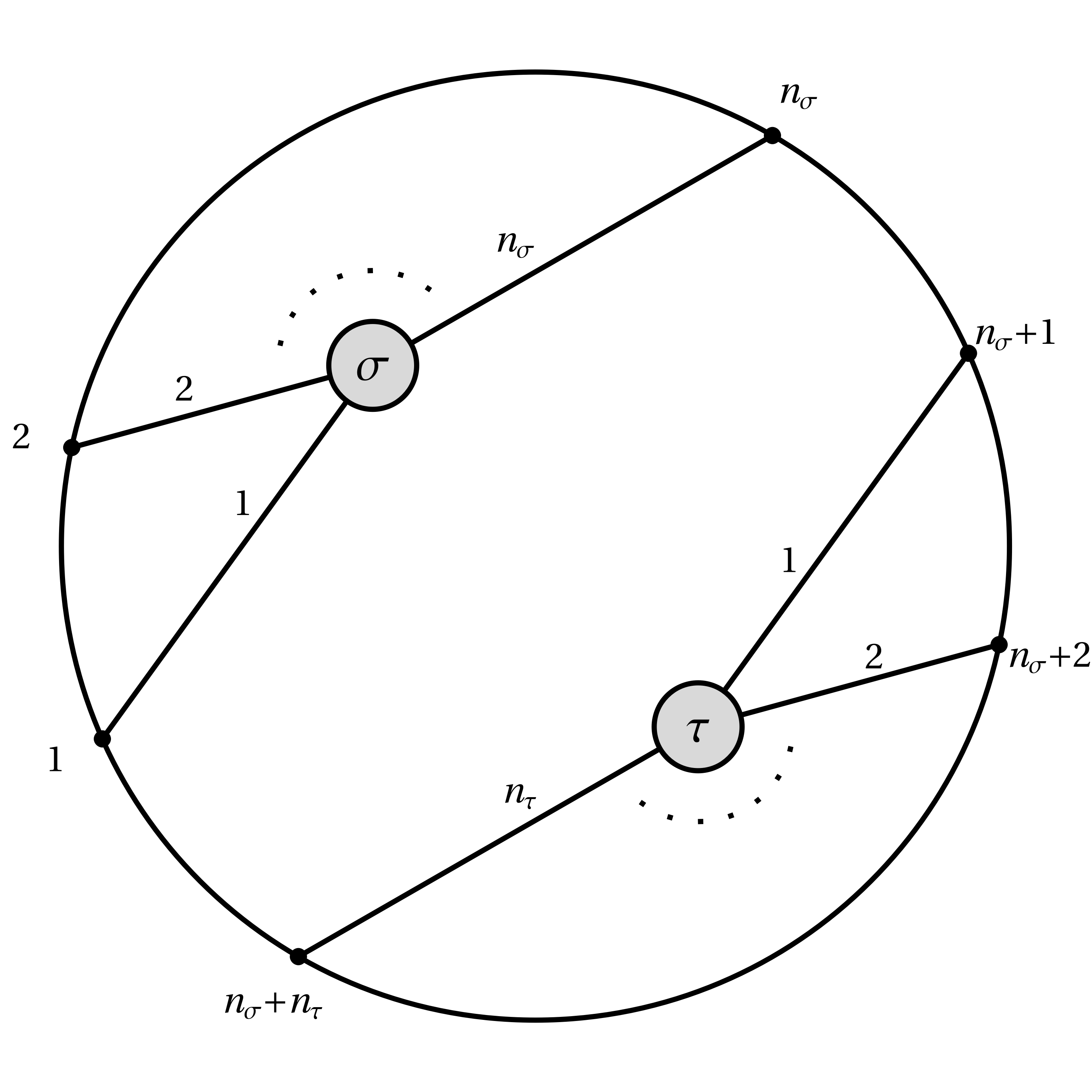
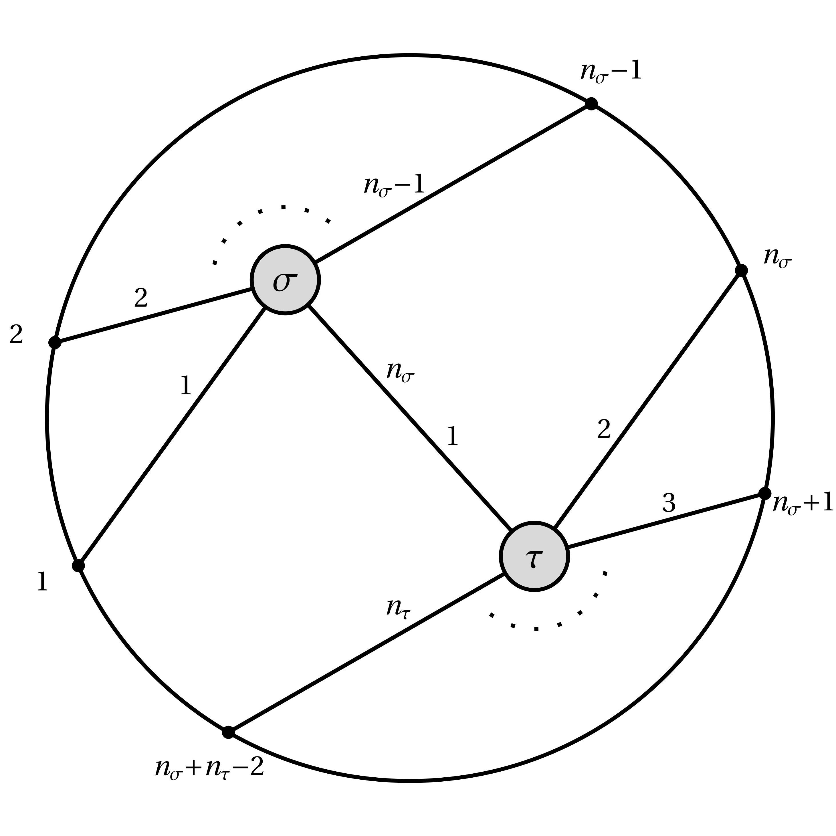
Figure 5. Direct sum (left) and amalgamation (right) of two permutations $\sigma$ on $n_{\sigma}$ letters and $\tau$ on $n_{\tau}$ letters.

Let us now interpret Theorem 3.37 in terms of permutations. We first need to describe the decorated permutations that arise from contracted Grassmannian trees and graphs.

For $n\geq 2$ and $1\leq k\leq n-1$, let

$$\pi_{k,n}\coloneqq(k+1,\ldots,n,1,2,\ldots,k)=\begin{pmatrix}1&2&\cdots&n-k&n-k+1&\cdots&n\\ \downarrow&\downarrow&&\downarrow&\downarrow&&\downarrow\\ k+1&k+2&\cdots&n&1&\cdots&k\end{pmatrix},$$

and for $n=1$, let $\pi_{0,1}\coloneqq(\underline{1})$ and $\pi_{1,1}\coloneqq(\overline{1})$ be the two decorated permutations on one letter decorated black and white, respectively.

Definition 4.7.

Given permutations $\sigma$ on $n_{\sigma}$ letters and $\tau$ on $n_{\tau}$ letters, where $n_{\sigma},n_{\tau}\geq 2$, the amalgamation $\sigma\star\tau$ is a permutation on $n_{\sigma}+n_{\tau}-2$ letters defined as follows:

$$(\sigma\star\tau)(i)\coloneqq\left\{\begin{array}[]{ll}\sigma(i)&\text{if $1\leq i\leq n_{\sigma}-1$ and $\sigma(i)\neq n_{\sigma}$,}\\ \tau(1)&\text{if $1\leq i\leq n_{\sigma}-1$ and $\sigma(i)=n_{\sigma}$,}\\ \tau(i-n_{\sigma}+2)&\text{if $n_{\sigma}\leq i\leq n_{\sigma}+n_{\tau}-2$ and $\tau(i-n_{\sigma}+2)\neq 1$,}\\ \sigma(n_{\sigma})&\text{if $n_{\sigma}\leq i\leq n_{\sigma}+n_{\tau}-2$ and $\tau(i-n_{\sigma}+2)=1$.}\end{array}\right.$$ (4.12)

This operation is illustrated in Figure 5 (right).

Definition 4.13.

The cyclic rotation of a permutation $\pi=(\pi_{1},\ldots,\pi_{n-1},\pi_{n})$ is the permutation $\text{cyc}(\pi)$ defined by $(\text{cyc}(\pi))(i)\coloneqq\pi(i-1)+1$, i.e. $\text{cyc}(\pi)=(\pi_{n}+1,\pi_{1}+1,\ldots,\pi_{n-1}+1)$ (modulo $n$).

The above operation corresponds to taking a decorated permutation arising from a Grassmannian graph on vertices $1,2,\dots,n$, then adding $1$ (modulo $n$) to each boundary vertex and computing the new decorated permutation.

Definition 4.14.

A Grassmannian tree permutation is a permutation built by amalgamating permutations of the form $\pi_{k,n}$ (for $n\geq 3$) and possibly applying cyclic rotations. We also consider the permutations $(1)$ and $(2,1)$ on one and two letters, respectively, to be Grassmannian tree permutations.

The following statement is easy to verify from the definitions.

Proposition 4.15.

Grassmannian tree permutations are precisely the decorated permutations obtained from Grassmannian trees by applying the map from Definition 4.1.

Now we obtain from Theorem 3.37 the following corollary.

Corollary 4.16.

The number of Grassmannian tree permutations on $n$ letters with $k$ antiexcedances and momentum amplituhedron $r$ is given by $[x^{n}y^{k}q^{r}]\mathcal{G}_{\text{tree}}(x,y,q)$ where $\mathcal{G}_{\text{tree}}(x,y,q)$ is as in Theorem 3.37.

One can also interpret Theorem 3.37 as enumerating “Grassmannian forest permutations,” which are built from Grassmannian tree permutations by using the direct sum and cyclic rotation operations.

5. The Momentum Amplituhedron

Remarkably, the totally nonnegative Grassmannian underpins the structure of scattering amplitudes in planar $\mathcal{N}=4$ supersymmetric Yang-Mills (SYM) theory [AHBC⁺16]. In 2013, the (tree) amplituhedron $\mathcal{A}_{n,k,m}$ was introduced as a geometric object which encodes tree-level scattering amplitudes for $\mathcal{N}=4$ SYM in momentum twistor space [AHT14]. It is defined as the image of the totally nonnegative Grassmannian under a linear map induced by a positive matrix. Then in 2019, the momentum amplituhedron $\mathcal{M}_{n,k}=\mathcal{M}_{n,k,4}$ was discovered as an analogue of the amplituhedron but defined in momentum space [DFŁP19]. Like the amplituhedron, the momentum amplituhedron is defined as the image of the totally nonnegative Grassmannian under a particular map. Its boundary stratification was extensively studied in [FŁM20] and a (conjectural) description for its boundaries was given in terms of Grassmannian forests, although these objects were not known to the authors then. Moreover, each instance of the momentum amplituhedron computed in [FŁM20] was shown to have Euler characteristic $1$. In this section, we use the results of the previous section to construct the full generating function for the momentum amplituhedron and we prove that its Euler characteristic is $1$.

5.1. The momentum amplituhedron and its boundary stratification

Definition 5.1.

Define the twisted nonnegative part of $\operatorname{Gr}_{k,n}$ to be:

$$\operatorname{Gr}^{\geq 0,\tau}_{k,n}=\{V\in\operatorname{Gr}_{k,n}:(-1)^{\mbox{inv}(I,[n]\setminus I)}\Delta_{[n]\setminus I}(V)\geq 0\text{ for all }I\in{[n]\choose n-k}\}\,,$$ (5.2)

where $\mbox{inv}(A,B)=\#\{a\in A,b\in B|a>b\}$ denotes the inversion number.

One can verify as in [Kar17, Lemma 1.11] that if $\{\Delta_{I}(V)\}$ are the Plücker coordinates of a point $V$ in $\operatorname{Gr}_{k,n}$, then the orthogonal complement $V^{\perp}\in\operatorname{Gr}_{n-k,n}$ is represented by a point with Plücker coordinates $\Delta_{J}(V^{\perp})=(-1)^{\mbox{inv}(J,[n]\setminus J)}\Delta_{[n]\setminus J}(V)$ for $J\in{[n]\choose n-k}$.

Definition 5.3.

For $n,p$ with $n\geq p$, define $\mbox{Mat}^{>0}_{n,p}$ to be the set of real $n\times p$ matrices whose maximal minors (Plücker coordinates) are all positive and its twisted totally positive part as

$$\mbox{Mat}^{>0,\tau}_{n,p}=\{A\in\mbox{Mat}_{n,p}:(-1)^{\mbox{inv}(I,[n]\setminus I)}\Delta_{[n]\setminus I}(A)>0\text{ for all }I\in{[n]\choose n-p}\}\,.$$ (5.4)

Definition 5.5.

A subset $I$ of $[n]$ is said to be cyclically consecutive if its elements, or the elements of its complement in $[n]$, are consecutive.

Definition 5.6 ([DFŁP19, Section 2.2]).

Let $k,n$ be integers with $2\leq k\leq n-2$. Let $\tilde{\Lambda}\in\mbox{Mat}^{>0}_{n,k+2}$ and $\Lambda\in\mbox{Mat}^{>0,\tau}_{n,n-k+2}$ be a pair of matrices, called the kinematic data. Given an element $[C]\in\operatorname{Gr}_{k,n}^{\geq 0}$, with orthogonal complement $[C^{\perp}]\in\operatorname{Gr}_{n-k,n}$, let $\widetilde{Y}=C\tilde{\Lambda}$ and $Y=C^{\perp}\Lambda$. The momentum amplituhedron map $\Phi_{\tilde{\Lambda},\Lambda}:\operatorname{Gr}^{\geq 0}_{k,n}\rightarrow\operatorname{Gr}_{k,k+2}\times\operatorname{Gr}_{n-k,n-k+2}$ is defined by $\Phi_{\tilde{\Lambda},\Lambda}(C)\coloneqq(\widetilde{Y},Y)$ and the momentum amplituhedron $\mathcal{M}_{n,k}(\tilde{\Lambda},\Lambda)$ is the image of $\operatorname{Gr}_{k,n}^{\geq 0}$ under $\Phi_{\tilde{\Lambda},\Lambda}$.

For $i,j\in[n]$, we define $[\widetilde{Y}ij]=\det(\widetilde{Y}_{1},\ldots,\widetilde{Y}_{k},\tilde{\Lambda}_{i},\tilde{\Lambda}_{j})$ to be the determinant of the $(k+2)\times(k+2)$ matrix with rows $\widetilde{Y}_{1},\ldots,\widetilde{Y}_{k},\tilde{\Lambda}_{i},\tilde{\Lambda}_{j}$, and we define $\langle Yij\rangle=\det(Y_{1},\ldots,Y_{n-k},\Lambda_{i},\Lambda_{j})$ to be the determinant of the $(n-k+2)\times(n-k+2)$ matrix with rows $Y_{1},\ldots,Y_{n-k},\Lambda_{i},\Lambda_{j}$. We require that the kinematic data satisfy $\sum_{i<j\in I}[\widetilde{Y}ij]\langle Yij\rangle>0$ on $\operatorname{Gr}_{k,n}^{>0}$ for every cyclically consecutive subset $I$ of $[n]$ with $|I|\geq 2$; this is a necessary condition for the codimension-one boundaries of the momentum amplituhedron to correspond to factorization channels of the scattering amplitude [DFŁP19, Section 2.3].

While $\operatorname{Gr}_{k,k+2}\times\operatorname{Gr}_{n-k,n-k+2}$ has dimension $2n$, $\mathcal{M}_{n,k}$ has dimension $2n-4$.

Remark 5.7.

The combinatorial properties of $\mathcal{M}_{n,k}(\tilde{\Lambda},\Lambda)$ are conjectured to be independent of the choice of $(\tilde{\Lambda},\Lambda)$. Consequently, we will omit our choice and simply write $\mathcal{M}_{n,k}$.

Definition 5.8.

Given a positroid cell $S_{\sigma}$ (resp., $S_{G}$) of $\operatorname{Gr}_{k,n}^{\geq 0}$, we write $\Phi_{\sigma}^{\circ}=\Phi(S_{\sigma})$ (resp., $\Phi_{G}^{\circ}=\Phi(S_{G})$) and $\Phi_{\sigma}=\overline{\Phi(S_{\sigma})}$ (resp., $\Phi_{G}=\overline{\Phi(S_{G})}$), omitting our choice of kinematic data following Remark 5.7. We refer to $\Phi_{\sigma}^{\circ}$ (resp., $\Phi_{G}^{\circ}$) as a stratum of $\mathcal{M}_{n,k}$ and we denote its dimension by $\dim\Phi_{\sigma}^{\circ}$ (resp., $\dim\Phi_{G}^{\circ}$).

The following definition first appeared in [Łuk19, Section 2.4].

Definition 5.9.

Let $S_{\sigma_{k,n}}$ denote the unique top-dimensional positroid cell of $\operatorname{Gr}_{k,n}^{\geq 0}$ which is the interior of $\operatorname{Gr}_{k,n}^{\geq 0}$. Given a positroid cell $S_{\sigma}$ of $\operatorname{Gr}_{k,n}^{\geq 0}$, we say that $\Phi^{\circ}_{\sigma}$ is a boundary stratum (or simply boundary) of $\mathcal{M}_{n,k}$ if

• $\Phi^{\circ}_{\sigma}\cap\Phi^{\circ}_{\sigma_{k,n}}=\emptyset$, and

• for any positroid cell $S_{\sigma^{\prime}}$ whose closure contains $S_{\sigma}$, we have $\dim\Phi^{\circ}_{\sigma^{\prime}}>\dim\Phi^{\circ}_{\sigma}$.

The boundary stratification of the momentum amplituhedron was extensively studied in [FŁM20] using amplituhedronBoundaries.m [ŁM21], a Mathematica package. The package employs a recursive routine, initially developed for the $m=2$ amplituhedron in [Łuk19], which exploits the positroid stratification of $\operatorname{Gr}_{k,n}^{\geq 0}$. The algorithm in [Łuk19] (conjecturally) generates all boundaries as per the above definition.

Let $\mathcal{S}_{n,k}$ denote the set of decorated permutations $\sigma$ such that $\Phi^{\circ}_{\sigma}$ is a boundary stratum of $\mathcal{M}_{n,k}$, together with ${\sigma_{k,n}}$. Based on poset data generated in [FŁM20], we are emboldened to conjecture the following.

Conjecture 5.10.

We have a regular CW decomposition

$$\mathcal{M}_{n,k}=\sqcup_{\sigma\in\mathcal{S}_{n,k}}\Phi^{\circ}_{\sigma}$$

of the momentum amplituhedron. In particular, each boundary stratum $\Phi^{\circ}_{\sigma}$ is homeomorphic to an open ball.

The authors of [FŁM20] synthesised the boundary stratification of $\mathcal{M}_{n,k}$ for $4\leq n\leq 8$ and $2\leq k\leq n-2$. From this data, they observed that positroid cells corresponding to momentum amplituhedron boundaries are labelled by Grassmannian forests. Combining their observations with knowledge about the singularity structure of tree-level amplitudes in $\mathcal{N}=4$ SYM, they hypothesised a bijection between boundaries and the aforementioned pictorial labels. This hypothesis is summarised below.

Conjecture 5.11 ([FŁM20, Section 3.3]).

$\Phi_{G}^{\circ}$ is a boundary of $\mathcal{M}_{n,k}$ if and only if $G$ is a Grassmannian forest of type $(k,n)$. Moreover, given a Grassmannian forest $F$, $\dim\Phi_{F}^{\circ}=\dim_{\mathcal{M}}(F)$.

Remark 5.12.

It is immediate from the definition that the momentum amplituhedron $\mathcal{M}_{n,2}$ is isomorphic to $\operatorname{Gr}^{\geq 0}_{2,n}$, and the boundary stratification of $\mathcal{M}_{n,2}$ coincides with the boundary stratification of $\operatorname{Gr}^{\geq 0}_{2,n}$.

5.2. Enumerating the boundaries of the momentum amplituhedron

From 5.11, the boundaries of the momentum amplituhedron $\mathcal{M}_{n,k}$ of dimension $r$ are in bijection with the contracted Grassmannian forests of type $(k,n)$ with mom-dimension $r$, whose generating function was given in Theorem 3.37. We summarise this result below.

Corollary 5.13.

The number of boundaries of the momentum amplituhedron $\mathcal{M}_{n,k}$ of dimension $r$ is given by $[x^{n}y^{k}q^{r}]\mathcal{G}_{\text{forest}}(x,y,q)$ where

$$x\mathcal{G}_{\text{forest}}(x,y,q)=\left(\frac{x}{1+\mathcal{G}_{\text{tree}}(x,y,q)}\right)^{\langle-1\rangle},$$

was computed in Theorem 3.37 and the compositional inverse is with respect to the variable $x$. Equivalently,

$$[x^{n}]\mathcal{G}_{\text{forest}}(x,y,q)=\frac{1}{n+1}[x^{n}]\left(1+\mathcal{G}_{\text{tree}}(x,y,q)\right)^{n+1}.$$

In the above expressions, we have from Theorem 3.37 that

$$\mathcal{G}_{\text{tree}}(x,y,q) =x\left(1+y+yq\,C^{\langle-1\rangle}(x,y,q)\right),\text{ with }$$

$$C(x,y,q) =\frac{x(1-x(1+y)q^{2}-x^{2}yq^{2}(1+q-q^{2})-x^{4}y^{2}q^{5}(1+q))}{(1+xq)(1+xyq)(1-xq^{2})(1-xyq^{2})}.$$

We have checked that this formula reproduces all results for $[x^{n}y^{k}]\mathcal{G}_{\text{forest}}(x,y,q)$ listed in Tables 1 and 2 of [FŁM20]. Their results include as high as $(n,k)=(12,2)$. In LABEL:tbl:G-forest we present $[x^{n}y^{k}]\mathcal{G}_{\text{forest}}(x,y,q)$ for $n=4$ through $12$ and for all $2\leq k\leq\lfloor\frac{n}{2}\rfloor$.

The following corollaries are predicated upon 5.11. Corollary 5.15 additionally requires 5.10.

Corollary 5.14.

The number of $0$-dimensional boundary strata of $\mathcal{M}_{n,k}$ is ${n\choose k}$, that is, $[x^{n}y^{k}q^{0}]\mathcal{G}_{\text{forest}}(x,y,q)={n\choose k}$.

Corollary 5.15.

The Euler characteristic of the momentum amplituhedron is $1$.

Proof of Corollary 5.15.

Recall that for a CW complex, the Euler characteristic is defined as the alternating sum $\chi=n_{0}-n_{1}+n_{2}-n_{3}+\ldots$ where $n_{r}$ denotes the number of cells of dimension $r$ in the complex. The Euler characteristic of $\mathcal{M}_{n,k}$ can be computed as $[x^{n}y^{k}]\mathcal{G}_{\text{forest}}(x,y,-1)$. To this end, let us specialize to $q=-1$ for $\mathcal{G}_{\text{tree}}(x,y,q)$ given in the expression (3.38) from Theorem 3.37. One can easily verify that

$$C(x,y,-1)=\frac{x}{(1-x)(1-xy)},$$ (5.16)

and that its compositional inverse with respect to the variable $x$ is given by

$$C^{\langle-1\rangle}(x,y,-1)=\frac{1+x(1+y)-\sqrt{\Delta}}{2xy},$$ (5.17)

where $\Delta=(1+x(1+y))^{2}-4x^{2}y$. Therefore we have that

$$\mathcal{G}_{\text{forest}}(x,y,-1) =\frac{1}{x}\left(\frac{x}{1+\mathcal{G}_{\text{tree}}(x,y,-1)}\right)^{\langle-1\rangle}$$

$$=\frac{1}{x}\left(\frac{x}{1+x(1+y)-\frac{1}{2}(1+x(1+y)-\sqrt{\Delta})}\right)^{\langle-1\rangle}$$

$$=\frac{1}{x}\left(\frac{2x}{1+x(1+y)+\sqrt{\Delta}}\right)^{\langle-1\rangle}$$

$$=\frac{1}{x}\left(\frac{1+x(1+y)-\sqrt{\Delta}}{2xy}\right)^{\langle-1\rangle}$$

$$=\frac{1}{x}C(x,y,-1)=\frac{1}{(1-x)(1-xy)}=\sum_{0\leq n}x^{n}\sum_{0\leq k\leq n}y^{k},$$

with every coefficient equal to $1$. ∎

Appendix A Data

In LABEL:tbl:G-forest we give expressions for $[x^{n}y^{k}]\mathcal{G}_{\text{forest}}(x,y,q)$ for $4\leq n\leq 12$, which extends the range of data presented in Tables 1 and 2 of [FŁM20]. Since the number of contracted Grassmannian forests of type $(k,n)$ equals those of type $(n-k,n)$ (see Remark 3.20) we restrict $k$ to $2\leq k\leq\lfloor\frac{n}{2}\rfloor$.

Table 1. Expressions for $[x^{n}y^{k}]\mathcal{G}_{\text{forest}}(x,y,q)$ for $4\leq n\leq 12$ and $2\leq k\leq\lfloor\frac{n}{2}\rfloor$.

$(n,k)$	$[x^{n}y^{k}]\mathcal{G}_{\text{forest}}(x,y,q)$
$(4,2)$	$q^{4}+4q^{3}+10q^{2}+12q+6$
$(5,2)$	$q^{6}+5q^{5}+15q^{4}+30q^{3}+40q^{2}+30q+10$
$(6,2)$	$q^{8}+6q^{7}+21q^{6}+50q^{5}+90q^{4}+120q^{3}+110q^{2}+60q+15$
$(6,3)$	$q^{8}+15q^{7}+54q^{6}+114q^{5}+180q^{4}+215q^{3}+180q^{2}+90q+20$
$(7,2)$	$q^{10}+7q^{9}+28q^{8}+77q^{7}+161q^{6}+266q^{5}+350q^{4}+350q^{3}+245q^{2}+105q+21$
$(7,3)$	$q^{10}+21q^{9}+119q^{8}+350q^{7}+665q^{6}+938q^{5}+1050q^{4}+910q^{3}+560q^{2}+210q+35$
$(8,2)$	$q^{12}+8q^{11}+36q^{10}+112q^{9}+266q^{8}+504q^{7}+784q^{6}+1008q^{5}+1050q^{4}+840q^{3}+476q^{2}+168q+28$
$(8,3)$	$q^{12}+28q^{11}+188q^{10}+720q^{9}+1820q^{8}+3262q^{7}+4424q^{6}+4788q^{5}+4200q^{4}+2870q^{3}+1400q^{2}+420q+56$
$(8,4)$	$q^{12}+32q^{11}+300q^{10}+1280q^{9}+3264q^{8}+5696q^{7}+7420q^{6}+7672q^{5}+6426q^{4}+4200q^{3}+1960q^{2}+560q+70$
$(9,2)$	$q^{14}+9q^{13}+45q^{12}+156q^{11}+414q^{10}+882q^{9}+1554q^{8}+2304q^{7}+2898q^{6}+3066q^{5}+2646q^{4}+1764q^{3}+840q^{2}+252q+36$
$(9,3)$	$q^{14}+36q^{13}+279q^{12}+1227q^{11}+3726q^{10}+8370q^{9}+14322q^{8}+19152q^{7}+20622q^{6}+18270q^{5}+13230q^{4}+7476q^{3}+3024q^{2}+756q+84$
$(9,4)$	$q^{14}+45q^{13}+540q^{12}+3003q^{11}+10089q^{10}+23049q^{9}+38298q^{8}+48618q^{7}+49140q^{6}+40656q^{5}+27468q^{4}+14490q^{3}+5460q^{2}+1260q+126$
$(10,2)$	$q^{16}+10q^{15}+55q^{14}+210q^{13}+615q^{12}+1452q^{11}+2850q^{10}+4740q^{9}+6765q^{8}+8340q^{7}+8862q^{6}+7980q^{5}+5880q^{4}+3360q^{3}+1380q^{2}+360q+45$
$(10,3)$	$q^{16}+45q^{15}+395q^{14}+1955q^{13}+6705q^{12}+17412q^{11}+35640q^{10}+58440q^{9}+77490q^{8}+84120q^{7}+75852q^{6}+57120q^{5}+35280q^{4}+17010q^{3}+5880q^{2}+1260q+120$
$(10,4)$	$q^{16}+60q^{15}+880q^{14}+5780q^{13}+23385q^{12}+65990q^{11}+137835q^{10}+220662q^{9}+277890q^{8}+281940q^{7}+235410q^{6}+163380q^{5}+92862q^{4}+41160q^{3}+13020q^{2}+2520q+210$
$(10,5)$	$q^{16}+65q^{15}+1045q^{14}+7915q^{13}+34740q^{12}+101240q^{11}+212285q^{10}+336220q^{9}+415890q^{8}+412980q^{7}+336840q^{6}+228102q^{5}+126420q^{4}+54600q^{3}+16800q^{2}+3150q+252$
$(11,2)$	$q^{18}+11q^{17}+66q^{16}+275q^{15}+880q^{14}+2277q^{13}+4917q^{12}+9042q^{11}+14355q^{10}+19855q^{9}+24057q^{8}+25542q^{7}+23562q^{6}+18480q^{5}+11880q^{4}+5940q^{3}+2145q^{2}+495q+55$
$(11,3)$	$q^{18}+55q^{17}+539q^{16}+2959q^{15}+11275q^{14}+32692q^{13}+75735q^{12}+143913q^{11}+226908q^{10}+297990q^{9}+326997q^{8}+301620q^{7}+235158q^{6}+154308q^{5}+83160q^{4}+34980q^{3}+10560q^{2}+1980q+165$
$(11,4)$	$q^{18}+77q^{17}+1342q^{16}+10109q^{15}+46849q^{14}+153527q^{13}+380402q^{12}+738067q^{11}+1143780q^{10}+1435005q^{9}+1475562q^{8}+1259412q^{7}+901362q^{6}+540540q^{5}+265650q^{4}+101640q^{3}+27720q^{2}+4620q+330$
$(11,5)$	$q^{18}+88q^{17}+1782q^{16}+16522q^{15}+88924q^{14}+318197q^{13}+820512q^{12}+1602986q^{11}+2450437q^{10}+2996972q^{9}+2984520q^{8}+2457840q^{7}+1693230q^{6}+975744q^{5}+460152q^{4}+168630q^{3}+43890q^{2}+6930q+462$
$(12,2)$	$q^{20}+12q^{19}+78q^{18}+352q^{17}+1221q^{16}+3432q^{15}+8074q^{14}+16236q^{13}+28314q^{12}+43252q^{11}+58278q^{10}+69564q^{9}+73656q^{8}+68904q^{7}+56232q^{6}+39072q^{5}+22275q^{4}+9900q^{3}+3190q^{2}+660q+66$
$(12,3)$	$q^{20}+66q^{19}+714q^{18}+4300q^{17}+17985q^{16}+57420q^{15}+147202q^{14}+312378q^{13}+558855q^{12}+850575q^{11}+1104048q^{10}+1221682q^{9}+1152888q^{8}+929610q^{7}+640200q^{6}+372636q^{5}+178200q^{4}+66495q^{3}+17820q^{2}+2970q+220$
$(12,4)$	$q^{20}+96q^{19}+1950q^{18}+16532q^{17}+85875q^{16}+316728q^{15}+892496q^{14}+2000988q^{13}+3651945q^{12}+5494500q^{11}+6864858q^{10}+7162452q^{9}+6278283q^{8}+4653000q^{7}+2924460q^{6}+1546776q^{5}+670230q^{4}+225720q^{3}+54120q^{2}+7920q+495$
$(12,5)$	$q^{20}+114q^{19}+2808q^{18}+30694q^{17}+192327q^{16}+805833q^{15}+2456976q^{14}+5730414q^{13}+10553631q^{12}+15676199q^{11}+19057434q^{10}+19172604q^{9}+16115616q^{8}+11412324q^{7}+6835752q^{6}+3438204q^{5}+1413720q^{4}+450450q^{3}+101640q^{2}+13860q+792$
$(12,6)$	$q^{20}+120q^{19}+3120q^{18}+36312q^{17}+245007q^{16}+1084332q^{15}+3412852q^{14}+8072064q^{13}+14897368q^{12}+22010536q^{11}+26499066q^{10}+26335804q^{9}+21837585q^{8}+15242040q^{7}+8992236q^{6}+4451832q^{5}+1800414q^{4}+563640q^{3}+124740q^{2}+16632q+924$

Appendix B Algebraic Relations

The rank-generating functions for contracted Grassmannian trees and forests presented in Theorem 3.37 satisfy the following algebraic relations:

$$\autobreak 0=q(q+1)\mathcal{G}_{\text{tree}}^{5}+qx(q^{2}xy-5q(y+1)-5(y+1))\mathcal{G}_{\text{tree}}^{4}+x^{2}(q(-3q^{2}xy(y+1)+q(10-y((x-10)y+x-19))+y(10y+21)+10)+y)\mathcal{G}_{\text{tree}}^{3}+x^{3}(q^{3}xy(y(3y+7)+3)+q^{2}(y+1)(y(2(x-5)y+2x-17)-10)-q(y(y(-x+10y+32)+32)+10)-3y(y+1))\mathcal{G}_{\text{tree}}^{2}-x^{4}(q^{3}xy(y+1)(y(y+4)+1)+q^{2}(y+1)(y((x-5)y^{2}+3(x-4)y+x-12)-5)-q(y+1)(y(y(-x+5y+16)+16)+5)-y(y(3y+5)+3))\mathcal{G}_{\text{tree}}+x^{5}(q^{3}xy^{2}(y+1)^{2}-q^{2}(y+1)^{2}(y(y(-x+y+2)+2)+1)-q(y(y(y(-x+y(y+5)+10)+10)+5)+1)-y(y+1)(y^{2}+y+1))\,,$$ (B.1)

$$\autobreak 0=q(x-1)x^{2}y(xy-1)(q(xy+x-1)+x)(q(xy+x-1)+xy)\mathcal{G}_{\text{forest}}^{6}+(q^{3}x^{2}y(xy+x-1)(x(xy(y+4)+x-5(y+1))+4)+q^{2}(x(x(-(x^{3}(y+1)(y(y+2)(y^{2}+1)+1))+x^{2}(y+1)^{2}(y(5y+3)+5)-2x(y+1)(y(5y+7)+5)+y(10y+19)+10)-5(y+1))+1)-q(x^{2}(y^{2}+y+1)-2x(y+1)+1)(x(x(x(y+1)(y(y+3)+1)-y(3y+8)-3)+3(y+1))-1)-x^{2}y(xy+x-1)(x^{2}(y^{2}+y+1)-2x(y+1)+1))\mathcal{G}_{\text{forest}}^{5}+(q^{3}x^{2}y(x^{2}(y(3y+7)+3)-9x(y+1)+6)-q^{2}(x(x(5x^{2}(y+1)^{2}(y^{2}+y+1)-x(y+1)(y(20y+31)+20)+30y^{2}+57y+30)-20(y+1))+5)-q(x(x(x^{2}(y(y(y(5y+21)+31)+21)+5)-4x(y+1)(y(5y+11)+5)+30y^{2}+63y+30)-20(y+1))+5)-x^{2}y(x^{2}(y(3y+5)+3)-6x(y+1)+3))\mathcal{G}_{\text{forest}}^{4}+(-10q(q+1)x^{3}y^{3}+(q+1)x^{2}y^{2}((q(3q-29)-3)x+30q)+xy((q+1)(q(3q-29)-3)x^{2}+(q(q(57-4q)+63)+3)x-30q(q+1))-10q(q+1)(x-1)^{3})\mathcal{G}_{\text{forest}}^{3}+(q+1)(q^{2}x^{2}y-10q(xy+x-1)^{2}-x^{2}y)\mathcal{G}_{\text{forest}}^{2}-5q(q+1)(xy+x-1)\mathcal{G}_{\text{forest}}-q(q+1)\,.$$ (B.2)

References

- [AHBC+16] Nima Arkani-Hamed, Jacob L. Bourjaily, Freddy Cachazo, Alexander B. Goncharov, Alexander Postnikov, and Jaroslav Trnka. Grassmannian Geometry of Scattering Amplitudes. Cambridge University Press, 4 2016. arXiv:1212.5605, doi:10.1017/CBO9781316091548.
- [AHT14] Nima Arkani-Hamed and Jaroslav Trnka. The Amplituhedron. J. High Energy Phys., 10:030, 2014. arXiv:1312.2007, doi:10.1007/JHEP10(2014)030.
- [Ard15] Federico Ardila. Algebraic and geometric methods in enumerative combinatorics. Handbook of enumerative combinatorics, pages 589–678, 2015. arXiv:1409.2562, doi:10.1201/b18255-3.
- [BBL98] Prosenjit Bose, Jonathan F. Buss, and Anna Lubiw. Pattern matching for permutations. Information Processing Letters, 65(5):277–283, 1998. URL: https://www.sciencedirect.com/science/article/pii/S0020019097002093, doi:https://doi.org/10.1016/S0020-0190(97)00209-3.
- [BLL98] François Bergeron, Gilbert Labelle, and Pierre Leroux. Combinatorial species and tree-like structures. Number 67 in Encyclopedia of Mathematics and its Applications. Cambridge University Press, 1998. doi:10.1017/CBO9781107325913.
- [Bou12] Jacob L. Bourjaily. Positroids, Plabic Graphs, and Scattering Amplitudes in Mathematica. Preprint, 12 2012. arXiv:1212.6974.
- [DFŁP19] David Damgaard, Livia Ferro, Tomasz Łukowski, and Matteo Parisi. The Momentum Amplituhedron. J. High Energy Phys., 08:042, 2019. arXiv:1905.04216, doi:10.1007/JHEP08(2019)042.
- [Dra08] Brian Drake. An inversion theorem for labeled trees and some limits of areas under lattice paths. Ph.D. Thesis, Brandeis University, 2008. URL: https://people.brandeis.edu/~gessel/homepage/students/drakethesis.pdf.
- [FŁM20] Livia Ferro, Tomasz Łukowski, and Robert Moerman. From momentum amplituhedron boundaries toamplitude singularities and back. J. High Energy Phys., 07(07):201, 2020. arXiv:2003.13704, doi:10.1007/JHEP07(2020)201.
- [FLZ18] Shishuo Fu, Zhicong Lin, and Jiang Zeng. On two unimodal descent polynomials. Discrete Mathematics, 341(9):2616–2626, 2018. URL: https://www.sciencedirect.com/science/article/pii/S0012365X1830181X, doi:https://doi.org/10.1016/j.disc.2018.06.010.
- [JKM17] David Jackson, Achim Kempf, and Alejandro Morales. A robust generaliztion of the legendre transform for qft. J. Phys. A: Mathemtical and Theoretical, (50), 2017.
- [Kar17] Steven N. Karp. Sign variation, the Grassmannian, and total positivity. J. Combin. Theor., Series A145:308–339, 2017. arXiv:1503.05622, doi:10.1016/j.jcta.2016.08.003.
- [Kit11] Sergey Kitaev. Patterns in permutations and words, volume 1 of Monographs in Theoretical Computer Science. An EATCS Series. Springer, 2011. doi:10.1007/978-3-642-17333-2.
- [KW19] Steven N. Karp and Lauren K. Williams. The m=1 amplituhedron and cyclic hyperplane arrangements. Int. Math. Res. Not., 5:1401–1462, 2019. arXiv:1608.08288, doi:10.1093/imrn/rnx140.
- [ŁM21] Tomasz Łukowski and Robert Moerman. Boundaries of the amplituhedron with amplituhedronBoundaries. Comput. Phys. Commun., 259:107653, 2021. arXiv:2002.07146, doi:10.1016/j.cpc.2020.107653.
- [ŁPW20] Tomasz Łukowski, Matteo Parisi, and Lauren K. Williams. The positive tropical Grassmannian, the hypersimplex, and the m=2 amplituhedron. Preprint, 2 2020. arXiv:2002.06164.
- [Łuk19] Tomasz Łukowski. On the Boundaries of the m=2 Amplituhedron. Preprint, 8 2019. arXiv:1908.00386.
- [Lus94] George Lusztig. Total positivity in reductive groups. In Lie theory and geometry, volume 123 of Progress in Mathematics, pages 531–568. Birkhäuser Boston, Boston, MA, 1994. doi:10.1007/978-1-4612-0261-5_20.
- [Pos06] Alexander Postnikov. Total positivity, Grassmannians, and networks. Preprint, 9 2006. arXiv:math/0609764.
- [Pos18] Alexander Postnikov. Positive Grassmannian and polyhedral subdivisions. Preprint, 6 2018. arXiv:1806.05307.
- [PSBW21] Matteo Parisi, Melissa Sherman-Bennett, and Lauren Williams. The m=2 amplituhedron and the hypersimplex: signs, clusters, triangulations, Eulerian numbers. Preprint, 4 2021. arXiv:2104.08254.
- [PSW09] Alexander Postnikov, David Speyer, and Lauren Williams. Matching polytopes, toric geometry, and the totally non-negative Grassmannian. Journal of Algebraic Combinatorics, 30(2):173–191, 2009. doi:10.1007/s10801-008-0160-1.
- [SI22] Neil J. A. Sloane and The OEIS Foundation Inc. The On-Line Encyclopedia of Integer Sequences, 2022. Published electronically at https://oeis.org.
- [SP02] Richard P Stanley and Jim Pitman. A polytope related to empirical distributions, plane trees, parking functions, and the associahedron. Discrete & Computational Geometry, 27(4):603–602, 2002. doi:10.1007/s00454-002-2776-6.
- [Spe94] Roland Speicher. Multiplicative functions on the lattice of non-crossing partitions and free convolution. Mathematische Annalen, 298(4):611–628, 1994. doi:10.1007/BF01459754.
- [Sta99] Richard P. Stanley. Enumerative combinatorics. Volume 2, volume 62 of Cambridge Studies in Advanced Mathematics. Cambridge University Press, Cambridge, 1999. With a foreword by Gian-Carlo Rota and appendix 1 by Sergey Fomin. doi:10.1017/CBO9780511609589.
- [SW05] David Speyer and Lauren Williams. The tropical totally positive Grassmannian. Journal of Algebraic Combinatorics, 22(2):189–210, 2005. arXiv:math/0312297, doi:10.1007/s10801-005-2513-3.
- [SW16] Alison Schuetz and Gwyn Whieldon. Polygonal dissections and reversions of series. Involve, a Journal of Mathematics, 9(2):223–236, 2016. doi:10.2140/involve.2016.9.223.
- [Wil05] Lauren K Williams. Enumeration of totally positive Grassmann cells. Advances in Mathematics, 190(2):319–342, 2005. URL: https://www.sciencedirect.com/science/article/pii/S0001870804000544, doi:https://doi.org/10.1016/j.aim.2004.01.003.