Scaling and renormalization in the modern theory of polarization: application to disordered systems

Abstract

We develop a scaling theory and a renormalization technique in the context of the modern theory of polarization. The central idea is to use the characteristic function (also known as the polarization amplitude) in place of the free energy in the scaling theory and in place of the Boltzmann probability in a position-space renormalization scheme. We derive a scaling relation between critical exponents which we test in a variety of models in one and two dimensions. We then apply the renormalization to disordered systems. In one dimension the renormalized disorder strength tends to infinity indicating the entire absence of extended states. Zero(infinite) disorder is a repulsive(attractive) fixed point. In two and three dimensions, at small system sizes, two additional fixed points appear, both at finite disorder, $W_{a}$($W_{r}$) is attractive(repulsive) such that $W_{a}<W_{r}$. In three dimensions $W_{a}$ tends to zero, $W_{r}$ remains finite, indicating metal-insulator transition at finite disorder. In two dimensions we are limited by system size, but we find that both $W_{a}$ and $W_{r}$ decrease significantly as system size is increased.

I Introduction

Scaling theory of localization in disordered systems Abrahams79 ; Lee85 ; Evers08 ; Langedijk09 has a long history. A milestone work by Abrahams et al. Abrahams79 , often referred to as the “gang of four” paper (G4), put forth this theory to explain the dimensional dependence of criticality. The central results for systems of no symmetry are that all states are localized in one dimension (1D), even in two dimensions (2D) there are no extended states, but here a crossover occurs, and only in three dimensions (3D) does a true metal-insulator transition occur in the form of an unstable fixed point.

Experimental evidence shows unambiguous support for the G4 conclusions in 1D Billy08 ; Roati08 and 3D Kondov11 ; Jendrzejewski11 ; Semeghini15 . The 2D results were more difficult to establish White20 experimentally, due to the possibility of weak localization RobertdeSaintVincent10 ; Jendrzejewski12 ; Muller15 . Theoretically a debate Kuzovkov02 ; Markos04 ; Suslov05 about a possible metal-insulator transition in 2D, rather than the entire absence of extended states, arose.

An important development in the understanding of crystalline systems in general (with or without disorder) was the development of the modern theory of polarization King-Smith93 ; Resta94 ; Resta00 (MTP). This theory provides the tools Resta98 ; Resta99 to measure localization. Although some studies Bendazzoli10 ; Varma15 ; Olsen17 have used these tools to assess localization in disordered systems, how the G4 results concur with the MTP is still an open question.

In this paper we seek to fill this gap by developing thermodynamic scaling and renormalization methods Reichl16 ; Kadanoff66 ; Wilson71 within the MTP context. The idea is to use the MTP characteristic function (also known as the polarization amplitude Kobayashi18 ) in place of the partition function as a starting point for both scaling (similar to Widom scaling of critical exponents) and our position space renormalization scheme.

In 1D our flow lines tend to a high disorder attractive fixed point, meaning that there are no extended states. In 2D and 3D, for finite system sizes, we find an attractive ($W_{a}$) and a repulsive ($W_{r}$) fixed point ($W_{a}<W_{r}$). The key question becomes how these fixed points evolve with system size. In 3D $W_{a}$ tends to zero, while $W_{r}$ tends to a finite number, indicating a metal-insulator transition. In 2D both the $W_{a}$ and $W_{r}$ decrease, but due to finite size limitations it is difficult to draw a definite conclusion valid for the thermodynamic limit. We discuss the possible scenarios.

Other renormalization approaches to Anderson localized systems, apart from the G4 scaling theory, also have been used Domany79 ; Sarker81 ; Shapiro82 ; Foster09 . Traditional real-space renormalization schemes, based on blocking sites of the lattice (Migdal-Kadanoff procedure) concur with G4. In the context of MTP renormalization has been applied by Voit and Nakamura Nakamura02 , but this technique relies on bosonization and is only applicable in 1D.

There are many investigations Marzari12 ; Yahyavi17 ; Kobayashi18 ; Hetenyi19 ; Patankar18 ; Furuya19 which focus on the distribution function and the scaling of the polarization amplitude in band theoretic and correlated quantum models. MTP also serves as the starting point for deriving topological invariants Bernevig13 , for example, the time-reversal polarization, the topological invariant in the Fu-Kane spin-pump Fu06 is the difference of the Zak phases of different members of a Kramers pair.

In section II the scaling theory of localization and the MTP are outlined, and the motivation of this work is stated, also placing our work in contemporary context. In section III the Hamiltonians of the models studied in this work are given. In section IV we derive a relation between critical exponents based on Widom’s thermodynamic scaling and test it for some model systems. In section V we develop our renormalization approach and apply it to disordered systems in different dimensions. In section VI we conclude our work.

II Background and Motivation

The starting point of the G4 scaling theory Abrahams79 is the specification of the Thouless number Edwards72 as the relevant quantity to analyze. The Thouless number is a dimensionless conductance defined as

$$g(L)=\frac{G}{e^{2}/2\hbar},$$ (1)

where

$$G=\frac{\Delta E}{dE/dN},$$ (2)

where $\Delta E$ is the difference between energy levels calculated using periodic boundary conditions and anti-periodic boundary conditions, $dE/dN$ is the average level spacing. The argument in support of $G$ as a conductance is that it is localization that determines whether a state is insulating or not. A delocalized state should be sensitive to changing the boundary conditions, whereas a localized one should not. G4 then argues that the $g(L)$ depends only on the system size. The scaling theory then analyzes the scaling function

$$\beta(g)=\frac{d\ln g}{d\ln L}.$$ (3)

In this function $L$ appears explicitly, since in disordered systems the system size dependence is more pronounced than in clean systems. Asymptotic analysis can be applied. When the conductance is small (states are localized), it is expected that

$$g=\exp(-L/\xi),$$ (4)

where $\xi$ denotes a correlation length. When extended states dominate, the conductance is expected to behave as

$$g=\sigma_{0}L^{d-2},$$ (5)

where $\sigma_{0}$ denotes the conductivity, and $d$ is the dimensionality of the system. From this information, by plotting $\beta(g)$ as a function of $\ln g$ the dimensional dependence of the critical behavior can be surmised. In 1D, all states are localized, since the function $\beta(g)$ is always negative, even as $\ln g$ goes to infinity. In 2D the curve is negative when $\ln g$ is negative, and it approaches zero as $\ln g$ goes to infinity, meaning that even in 2D the states are extended, however, in this case due to the crossover between exponential and logarithmic behavior, G4 predicts that experiments may detect a sharp mobility edge. In 3D, since the curve crosses $\beta(g)=0$, corresponding to an unstable fixed point, a metal-insulator transition is predicted.

Overall, in assessing a metal-insulator transition (in ordered or disordered) many-body quantum systems, the 1964 work of Kohn Kohn64 was a starting point. On the one hand, Kohn argued Kohn64 that assessing whether a system is metallic or insulating can be done by investigating the response of the system to twisting the boundary conditions. On the other hand, Kohn also pointed out that the localization of the center of mass of the charge distribution is the ultimate measure of whether a system is conducting or insulating. The two approaches are equivalent.

The central difficulty addressed by MTP was the ill-defined nature of the position operator in systems with periodic boundary conditions. This difficulty hindered the application of the hypothesis of Kohn Kohn64 in calculations for crystalline systems. The problem was overcome by casting the polarization in terms of a geometric phase Berry84 of the Zak Zak89 variety, which arises upon integrating across the Brillouin zone. Other relevant properties, such as the many-body generalization Resta98 of the polarization, and the variance thereof Resta99 were also derived. The program of Kohn Kohn64 was later realized through the MTP King-Smith93 ; Resta94 ; Resta00 ; Resta99 .

In the formalism of Resta and Sorella, the variance of the total position is cast Resta99 as

$$\chi^{(2)}=\sigma^{2}=-\frac{L^{2}}{2\pi^{2}}\mbox{Re}\ln Z_{1}$$ (6)

where

$$Z_{q}=\langle\Psi_{0}|\exp\left(i\frac{2\pi q}{L}\hat{X}\right)|\Psi_{0}\rangle,$$ (7)

and where $|\Psi_{0}\rangle$ denotes a quantum ground state, $q$ is an integer, and the total position operator is defined as

$$\hat{X}=\sum_{j=1}^{L}\hat{n}_{j}j,$$ (8)

where $\hat{n}_{j}$ is the density operator at site $j$. If $\sigma$ tends to infinity with system size, the system is metallic.

In this work we perform calculations for disordered systems in different dimensions based on MTP. Since the Thouless number is a measure of localization, we replace it with the the quantity from the MTP which can be taken as its analog,

$$g(L)\rightarrow 1-|Z_{1}|.$$ (9)

This is not an exact correspondence by any means. We justify it by first stating that the variance can be cast according to an approximation Hetenyi19 different from the one of Resta and Sorella,

$$\sigma^{2}=\frac{L^{2}}{2\pi^{2}}(1-|Z_{1}|).$$ (10)

This approximation has the advantage that in the limit of the Fermi sea ($Z_{1}=0$) $\sigma$ scales with system size linearly, which is expected on robust physical grounds. Furthermore, in Fig. 2(a), in the inset, we show the quantity $1-|Z_{1}|$ as a function of the Thouless number (defined as the sum over the absolute value of the difference in energy between periodic and anti-periodic boundary conditions, divided by the total energy difference), for a 1D system of $L=160$, and averaged over one hundred disorder realizations (replicas) (Hamiltonian in Eq. (11)). The function is monotonic, which also justifies our replacing of the Thouless number with $|Z_{1}|$ in our renormalization scheme (section V).

To perform the asymptotic analysis, the G4 scaling theory uses two pieces of information. In the small conductivity (large disorder) limit it is assumed that the conductivity localizes exponentially (Eq. (4)). In the opposite limit the conductance is related to the conductivity via the relation (Eq. (5)). In the latter, there appears to be no direct prescription to calculate the conductance based on a microscopic Hamiltonian. To phrase the question differently: given a disordered Hamiltonian for which we can calculate the eigenstates, how do we calculate the conductance? Which states do we consider? Should we consider a distribution of states? In our calculations below we will average the relevant quantities over all states. This amounts to a high-temperature approximation, since all states have the same contribution. The position operator we use Selloni87 ; Fois88 ; Ancilotto92 is a single-body one.

III Models

Most of this paper is devoted to disordered systems. The one-dimensional version of the disordered Hamiltonian we study can be written

$$\hat{H}=\sum_{i=1}^{L}\left[-t(\hat{c}_{i}^{\dagger}\hat{c}_{i+1}+\mbox{H.c.})+W\xi_{i}\hat{n}_{i}\right],$$ (11)

where $t$ denotes the hopping parameter (which will be taken as the unit of energy), $W$ indicates the disorder strength, and $\xi_{i}$ is a normal distributed random number. On the other hand, in the next section we also test the result of our Widom scaling theory for the Su-Schrieffer-Heeger Su79 (SSH) and Rice-Mele Rice82 (RM) models. The latter can be written,

$$\hat{H}=\sum_{i=1}^{L}\left[-(t+(-1)^{i}\delta t)(c_{i}^{\dagger}c_{i+1}+\mbox{H.c.})+\Delta(-1)^{i}\hat{n}_{i}\right],$$ (12)

where $\delta t$ denotes the alternation in hopping, and $\Delta$ denotes the strength of an alternating on-site potential. The SSH Hamiltonian is obtained by setting $\Delta=0$ in Eq. (12).

IV Widom scaling in the modern theory of polarization

We consider an $N$-electron system, one-dimensional for convenience, periodic in $L$. The discrete analog of the characteristic function is given in Eqs. (7) and (8). The expression for the average position in a many-body crystalline system given by Resta is

$$\langle X\rangle=\frac{L}{2\pi}\mbox{Im}\ln Z_{1},$$ (13)

which reduces to the Zak phase if $\Psi_{0}$ is a Slater determinant. The average position Resta98 (Eq. (13)) and the variance Resta99 (Eq. (6)) are a finite difference derivatives of $\ln Z_{q}$ at $q=0$, first and second derivatives, respectively.

To our purposes in this section it is more suitable to take the thermodynamic limit in Eq. (7) and write

$$Z(K)=\langle\Psi_{0}|\exp\left(iK\hat{X}\right)|\Psi_{0}\rangle,$$ (14)

and express the variance as

$$\chi^{(2)}=-\left.\frac{\partial^{2}\ln Z(K)}{\partial K^{2}}\right|_{K=0}.$$ (15)

The quantity $\chi^{(2)}$ can be interpreted as a semi-classical approximation to the dielectric susceptibility. It is to be expected that if a phase transition point is approached from the insulating side $\chi^{(2)}$ diverges.

To keep the discussion general we introduce a variable $D$ which characterizes the approach to the critical point (we assume that $D=0$ is a quantum phase transition, or gap closure point). We first define

$$\chi^{(n)}(D,K)=\frac{1}{i^{n}}\frac{\partial^{n}\ln Z(D,K)}{\partial K^{n}},$$ (16)

and also define three critical exponents characterizing the approach to the phase transition:

$$\chi^{(2)}(D,0) \propto \frac{1}{D^{\beta}},$$ (17)

$$\chi^{(4)}(D,0) \propto \frac{1}{D^{\gamma}},$$

$$\chi^{(2)}(0,K) \propto \frac{1}{K^{\delta}}.$$

We also define the singular quantity,

$$\Phi(D,K)=-\ln Z(D,K),$$ (18)

which serves as the analog of the free energy. Applying the scaling relation $\Phi(\lambda^{a}D,\lambda^{b}K)=\lambda\Phi(D,K)$, we obtain the following relation between the scaling exponents:

$$\gamma\delta=\beta(\delta+2).$$ (19)

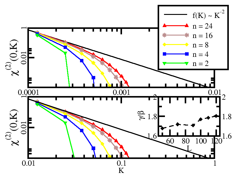
Figure 1: Log-log plot of $\chi^{(2)}(0,K)$ as a function of $K$ for different order finite difference approximations to the second derivative (see Eq. (16)) for two system sizes. $n$ refers to the order of the approximation, $\mathcal{O}(K^{-2n})$. The upper panel shows results for $L=100000$, the lower panel for $L=1000$. The solid line indicates a curve of the form $f(K)\propto K^{-2}$. The legend is for the upper and lower panels, not the inset of the lower panel. The inset of the lower panel shows the estimated ratio of the exponents $\gamma$ and $\beta$ as a function of system size for a two-dimensional disordered system.

We tested this relation on a number of different models. For the exponent $\delta$, ($D=0$ limit corresponds to the Fermi sea) our calculations are shown in Fig. 1. The different panels show different system sizes, the different curves within each panel are finite difference approximations to the second derivative (Eq. (17)). From these calculations we can conclude that $\delta=2$, which also means that $\gamma=2\beta$. We then calculated the other exponents of the SSH and Rice-Mele (Eq. (12)) models, in 1D and 2D, and found that $\beta=2$ and $\gamma=4$.

In addition, we also calculated the exponents for a 1D disordered system with the Hamiltonian given by Eq. (11). When calculating the cumulants (Eq. (17)) a difficulty faced was that a smooth curve only results for large systems. In particular, at small $W$, large system sizes are needed for converged results. We calculated the critical exponents for an $L=1280$ system, averaged over one hundred realizations of the disorder and found $\beta=3.61(5)$ and $\gamma=7.16(27)$, consistent with Eq. (19). We also made calculations for three different realizations of the disorder (three different calculations no disorder average is taken, only $W$ was swept) for a system of size $L=2560$. The results for the exponents turned out to be $\beta=3.53(4),3.45(4),3.52(5)$ and $\gamma=7.12(9),6.90(12),7.07(11)$, respectively, again consistent with Eq. (19) within error bars.

We also performed a calculation for a 2D disordered system. In this calculation we encountered system size related difficulties, however we provide an estimate of the ratios of critical exponents (inset of the lower panel of Fig. 1). As shown below, at the system sizes accessible, there is a transition in two-dimensional disordered systems (see Fig. 2), but the position of this transition decreases as system size is increased (see Fig. 4, upper panel). The relevant range of $\chi^{(2)}$ and $\chi^{(4)}$ as a function of $W$ is above the transition (which itself changes with system size), but before the disorder becomes too large, because then the errors are larger than the values of $\chi^{(2)}$ and $\chi^{(4)}$. We estimated the critical exponents $\gamma$ and $\beta$ by looking for the maxima of the derivatives of the functions $\log\chi^{(2)}$ and $\log\chi^{(4)}$ as a function of the logarithm of disorder strength. This estimate is shown in the inset of the lower panel of Fig. 1. The estimated ratio is increasing of the range of system sizes studied, and it is $\gamma/\beta\approx 1.8$ for the largest size, $L=120$.

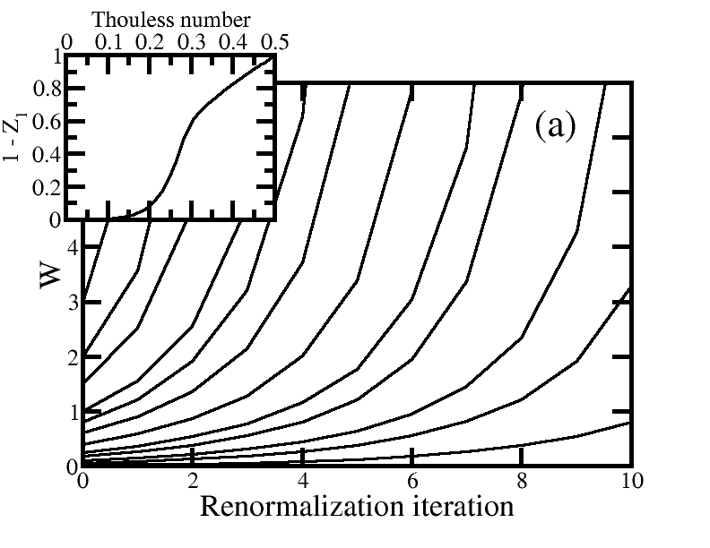
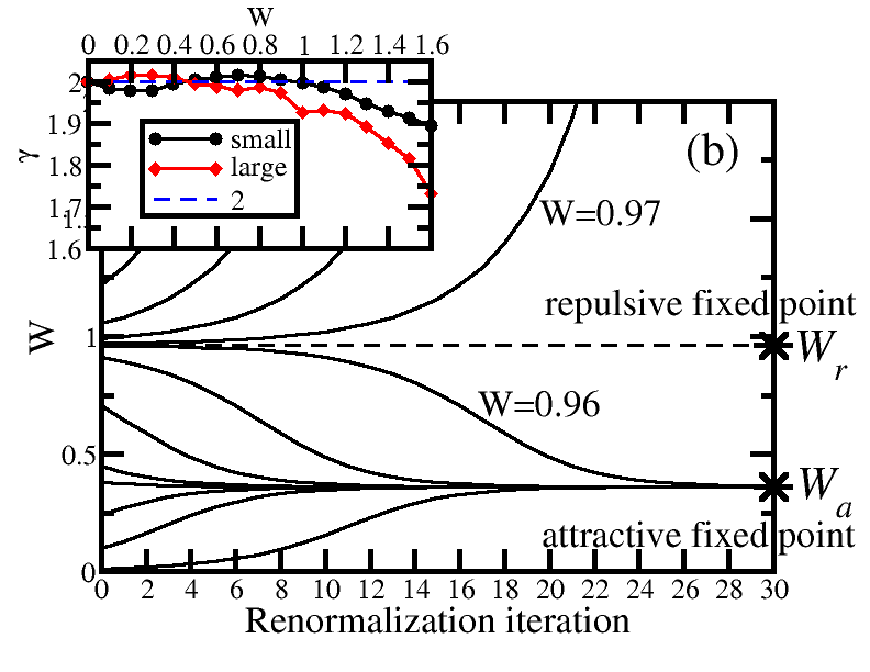
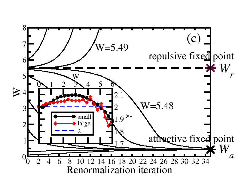
Figure 2: Renormalization flow lines for disordered systems of different dimensions. (a) One-dimensional $L=160$, 100 replicas averaged. The inset shows the quantity $1-Z_{1}$ vs. the Thouless number. (b) Two-dimensional, $L=24$, 100 replicas averaged. The repulsive ($W_{r}$) and attractive ($W_{a}$) fixed points are also indicated. The inset shows the size scaling exponent calculated using system sizes of $L=12,14,16,18$ (small) and $L=72,80,96$ (large). (c) Three-dimensional, $L=8$, 100 replicas averaged. The repulsive ($W_{r}$) and attractive ($W_{a}$) fixed points are also indicated. The inset shows the size scaling exponent calculated using system sizes of $L=6,8,10$ (small) and $L=20,22,24$ (large).

V Real-space renormalization in the modern theory of polarization

In real-space renormalization Reichl16 ; Kadanoff66 ; Wilson71 one starts with the blocking of sites of the lattice. To each block a single block variable is assigned. The blocked system is assumed to have the same Hamiltonian as the original Hamiltonian (although, this can mean an extended set of couplings). The parameters of the blocked Hamiltonian are tuned to produce the same Boltzmann probability as the original Hamiltonian, provided that the configurations of the starting Hamiltonian consistent with a given configuration of the block variables are summed over (traced out).

A common way to define a blocked system is by the procedure of “decimation”, in which some of the variables of the original system are traced out. In most cases the set of equations obtained this way are overdetermined, so either new parameters have to be introduced (for example, by extending the couplings included in the Hamiltonian) or via introducing further approximations, for example equating cumulants Niemeijer73 , between the original and the renormalized system, rather than the full Boltzmann distribution.

We now apply this set of steps to the quantity

$$\tilde{P}_{j}(x_{1},...,x_{L})=|\Psi_{0}(x_{1},...,x_{L})|^{2}\exp\left(i\frac{2\pi}{L}\hat{X}\right).$$ (20)

Here, the index $j$ indicates the step in the renormalization. As a first step we integrate out all the odd sites, resulting in

$$\tilde{P}_{j+1}(x_{2},...,x_{L})=\int.\int dx_{1}...dx_{L-1}\tilde{P}_{j}(x_{1},...,x_{L}).$$ (21)

We now require that the $\tilde{P}_{j}(x_{2},...,x_{L})$ of the remaining variables equals $\tilde{P}_{j+1}(x_{2},...,x_{L})$. It is easy to see, based on the definition of $\hat{X}$ (Eq. (8)), that $\tilde{P}_{j}(x_{2},...,x_{L})$ corresponds to the distribution of a system with half the size of the original one, $L/2$. As in other real-space renormalization techniques, the requirement is too stringent, so to arrive at a practical scheme, we use the relaxed requirement,

$$Z_{1}(W_{j+1},L/2)=Z_{1}(W_{j},L).$$ (22)

In other words, in each renormalization step, with a given disorder strength and system size, we find the disorder strength at half the system size which generates the same value of $Z_{1}(W_{j},L)$. It is not the entire probability distribution that is kept fixed in the course of a renormalization step, but only one Fourier mode of the distribution of the many-body position. In this sense, this renormalization is taylored to MTP.

In Fig. 2 the flowlines of the renormalization scheme are shown for systems of different dimensions. Fig. 3 shows the size scaling exponent ($\gamma$) of the variance of the polarization. We define $\gamma$ as

$$\chi^{(2)}=aL^{\gamma}.$$ (23)

In previous studies Hetenyi19 it was shown that metal-insulator transitions can be accurately determined by investigating $\gamma$. In clean systems a gapless system will exhibit $\gamma=2$, while in gapped insulators $\gamma\rightarrow 1$.

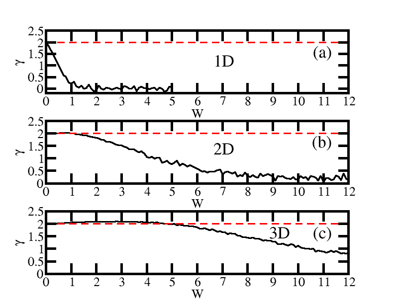
Figure 3: Size scaling exponent of the variance of the polarization for a (a) one-dimensional, (b) two-dimensional, and (c) three-dimensional system.

Fig. 2(a) shows results for a 1D disordered system of size $L=160$, and one hundred realizations of the disorder averaged. All flow lines which start at a finite value tend towards infinity indicating that all states are localized. We found no significant size dependence or dependence on the number of replicas. Also, the upper panel of Fig. 3(a) is consistent with the renormalization flows. The clean conducting system ($W=0$) exhibits $\gamma=2$, and finite disorder strength leads to a rapid decrease in $\gamma$. These results concur with the G4 Abrahams79 .

Fig. 2(b) shows the flowlines in a 2D sample calculation. The linear dimension of the system is $L=24$, the calculation was done on a square lattice. The number of disorder configurations averaged was one hundred. The flow lines here show qualitatively different behavior from the 1D case. We find two fixed points on the $W$ axis, one repulsive, $W_{r}\approx 1$, above which the flow lines tend to infinity, corresponding to a fully localized state. Below $W_{r}$, the flow lines which start at finite disorder strength tend to a finite disorder strength of $W_{a}$. $W_{r}$($W_{a}$) is a repulsive(attractive) fixed point. We have done a number of calculations and this qualitative behavior is maintained, however, we found variation in the values of $W_{r}$ and $W_{a}$. Fig. 3(b) shows the size scaling exponent in 2D. In these calculations system sizes up to $L=18$ ($L$ is the linear dimension) were used, and one hundred replicas were averaged. Note that until $W\approx 1$, the size scaling exponent is approximately two, above that value it decreases. The flow lines in 2(b) are consistent with the behavior of the scaling exponent.

Similar behavior is found in 3D, (see Figs. 2(c) and 3(c)). A repulsive fixed point $W_{r}$ and an attractive fixed point $W_{a}$ and $W_{r}>W_{a}$. The flow lines shown in Fig. 2(c) are for an $8\times 8\times 8$ system with 100 replicas averaged.

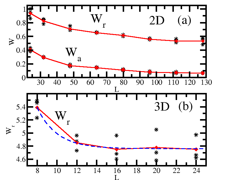
Figure 4: The behavior of fixed points as a function of system size in 2D and 3D. In 2D both the repulsive and the attractive fixed points are shown. The asterisks correspond to the raw data (three calculations) also shown in Tables 1 and 2. The red diamonds show the average of the three calculations for each system size. The blue dashed curve for 3D shows a fit function (see the text for a detailed discussion).

In the G4 scaling theory the system size itself appears as a relevant variable (Eq. (3)). For this reason, we further investigate the system size dependence of the attractive and repulsive fixed points. Our results are shown in Tables 1 and 2 and Fig. 4). To keep the CPU time manageable, we reduced the number of disorder configurations averaged, proportionately to system size. We made three calculations for each data point, and the raw data is shown in Tables 1 and 2. A plot is shown in Fig. 4, with the raw results and their average.

In 3D $W_{a}$ tends to zero, and $W_{r}$ approaches a finite value with large system size. The function fit in the lower panel of Fig. 4 is $f(L)=a\exp(bL)+c$, where $a=31.8259$, $b=-0.489526$ and $c=4.75641$. A metal-insulator transition takes place at finite $W_{r}$, in agreement with the G4 Abrahams79 . In 2D, due to finite size limitations, a definite conclusion is difficult to reach. Several scenarios are possible, depending on what happens to $W_{r}$ and $W_{a}$ as $L$ becomes large. Our results (upper panel, Fig. 4) show a sizeable decrease for both $W_{r}$ and $W_{a}$, $W_{r}\approx 1$ for the smallest size, and $W_{r}\approx 0.53$ for the largest one. Also, while $W_{a}$ does decrease, we can not say that it reaches zero (as it happens in 3D). There are then several possible scenarios. If $W_{a}$ and $W_{r}$ both go to zero, then extended states are absent, concurring with the G4. If only $W_{a}$ goes to zero, that would correspond to a metal-insulator transition, which would appear to be in accordance with transfer matrix and Lyapunov exponent based calculations Kuzovkov02 ; Suslov05 . A third possibility is that $W_{a}$ and $W_{r}$ both tend to finite values in the thermodynamic limit such that $W_{r}>W_{a}$. This would mean that there is a transition, but the small disorder states would be localized, rather than extended, even though, they would scale with system size as $L$ (substitute a finite size dependent $Z_{1}$ in Eq. (10)). We note that localized states of a qualitatively different nature, exhibiting power-law decay rather than exponential, have also been suggested Mott85 in 2D.

We also calculated $\gamma$ using different sets of systems, the results shown as insets in Fig. 2 middle and lower panel. In 2D we used systems with linear extension $L=12,16,18$($L=72,80,96$) for the data points designated “small”(“large”). For the former, $\gamma$ remains two up to $W\approx 1.0$, while for the latter, the decrease from two starts earlier at $W\approx 0.6$. In 3D increasing the system size does not lead to a similar decrease. (Here the linear extensions were $L=6,8,10$($L=20,22,24$) for “small”(“large”).) Although, these results are also limited by system size limitations, the suggestion is that when the system size is increased the curve in Fig. 3b eventually becomes like Fig. 3a, in other words, no sign of extended states remains, and our results likely concur with G4.

Size(No. of replicas)	$W_{r}(1)$	$W_{r}(2)$	$W_{r}(3)$	$W_{a}(1)$	$W_{a}(2)$	$W_{a}(3)$
$24\times 24$($100$)	$1.00$	$0.86$	$0.95$	$0.38$	$0.40$	$0.43$
$32\times 32$($50$)	$0.78$	$0.85$	$0.84$	$0.30$	$0.29$	$0.29$
$48\times 48$($25$)	$0.69$	$0.75$	$0.69$	$0.19$	$0.17$	$0.16$
$64\times 64$($15$)	$0.65$	$0.66$	$0.65$	$0.15$	$0.14$	$0.14$
$80\times 80$($10$)	$0.60$	$0.62$	$0.62$	$0.11$	$0.10$	$0.12$
$96\times 96$($5$)	$0.57$	$0.55$	$0.55$	$0.06$	$0.09$	$0.09$
$112\times 112$($4$)	$0.51$	$0.53$	$0.56$	$0.08$	$0.07$	$0.06$
$128\times 128$($3$)	$0.48$	$0.55$	$0.57$	$0.06$	$0.07$	$0.06$

Table 1: The repulsive ($W_{r}$) and attractive ($W_{a}$) fixed points for three sample calculations as a function of system size for a two-dimensional disordered system. The number of replicas is indicated in parentheses.

Size(No. of replicas)	$W_{r}(1)$	$W_{r}(2)$	$W_{r}(3)$	$W_{a}(1)$	$W_{a}(2)$	$W_{a}(3)$
$8\times 8\times 8$($100$)	$5.49$	$5.46$	$5.23$	$0.42$	$0.40$	$0.49$
$12\times 12\times 12$($25$)	$4.96$	$4.87$	$4.73$	$0.30$	$0.28$	$0.25$
$16\times 16\times 16$($10$)	$4.60$	$4.96$	$4.68$	$0.08$	$<0.01$	$0.23$
$20\times 20\times 20$($5$)	$5.05$	$4.70$	$4.58$	$<0.01$	$<0.01$	$0.05$
$24\times 24\times 24$($3$)	$4.62$	$4.97$	$4.66$	$<0.01$	$<0.01$	$<0.01$

Table 2: The repulsive ($W_{r}$) and attractive ($W_{a}$) fixed points for three sample calculations as a function of system size for a three-dimensional disordered system. The number of replicas is indicated in parentheses.

VI Conclusions

Wegner Wegner76 is credited Lee85 with introducing concepts from statistical mechanics into the study of disordered systems. In this work we applied statistical mechanical ideas using the characteristic function of the modern theory of polarization as a starting point. In particular we derived a scaling relation according to the steps followed by Widom to relate critical exponents, and we applied a renormalization procedure to the problem of disorder. In 1D and 3D our method is in full agreement with the common wisdom Abrahams79 on Anderson localized systems, however, in 2D we encountered system size limitations.

We note that the case of two dimensions has always been the most difficult one, both experimentally White20 ; RobertdeSaintVincent10 ; Jendrzejewski12 ; Muller15 and theoretically Kuzovkov02 ; Markos04 ; Suslov05 ; Mott85 ; Srivastava90 . Although, it is considered common knowledge that there are no extended states in two dimensions, the original work of Abrahams et al. Abrahams79 states that inspite of the absence of extended states, due to the crossover between exponential and logarithmic behavior, experiments may still detect a mobility edge.

References

- (1) E. Abrahams, P. W. Anderson, D. C. Licciardello, and T. V. Ramakrishnan, Phys. Rev. Lett. 42 673 (1979).
- (2) P. A. Lee and T. V. Ramakrishnan, Rev. Mod. Phys. 57 287 (1985).
- (3) F. Evers and A. D. Mirlin, Rev. Mod. Phys. 80 1355 (2008).
- (4) A. Langedijk, B. van Tieggelen, and D. S. Wiersma, Phys. Today 62 24 (2009).
- (5) J. Billy, V. Josse, Z. Zuo, A. Bernard, B. Hambrecht, P. Lugan, D. Clément, L. Sanchez-Palencia, P. Bouyer, and A. Aspect, Nature 453 891 (2008).
- (6) G. Roati, C. D’Errico, L. Fallani, M. Fattori, C. Fort, M. Zaccanti, G. Modugno, M. Modugno, and M. Inguscio, Nature 453 895 (2008).
- (7) S. S. Kondov, W. R. McGehee, J. J. Zibel, and B. DeMarco Science 334 66 (2011).
- (8) F. Jendrzejewski, A Bernard, K. Müller, P. Cheinet, V. Josse, M. Piraud, L. Pezzé, L. Sanchez-Palencia, A. Aspect, and P. Bouyer, Nat. Phys. 8 398 (2011).
- (9) G. Semeghini, M. Landini, P. Castilho, S. Roy, G. Spagnolli, A Trenkwalder, M. Fattori, M. Inguscio, and G. Modugno, Nat. Phys. 11 554 (2015).
- (10) D. H. White, T. A. Haase, D. J. Brown, M. D. Hoogerland, M. S. Najafabadi, J. L. Helm, C. Gies, D. Schumayer, and D. A. W. Hutchison, Nat. Comm. 11 4942 (2020).
- (11) M. Robert-de-Saint-Vincent, J.-P. Brantut, B. Allard, T. Plisson, L. Pezzé, L. Sanchez-Palencia, A. Aspect, T. Bourdel, and P. Bouyer, Phys. Rev. Lett. 104 220602 (2010).
- (12) F. Jendrzejewski, K. Müller, J. Richard, A. Date, T. Plisson, P. Bouyer, A. Aspect, and V. Josse, Phys. Rev. Lett. 109 195302 (2012).
- (13) K. Müller, J. Richard, V. V. Volchkov, V. Denechaud, P. Bouyer, A. Aspect, and V. Josse, Phys. Rev. Lett. 114 205301 (2015).
- (14) V. N. Kuzovkov, W. von Niessen, V. Kashcheyevs, O. Hein, J. Phys.: Cond. Mat. 14 13777 (2002).
- (15) P. Markoš, L. Schweitzer, and M. Weyrauch, J. Phys.: Cond. Mat. 16 1679 (2004).
- (16) I. M. Suslov, J. Exp. Theor. Phys. 101 661 (2005).
- (17) R. D. King-Smith and D. Vanderbilt, Phys. Rev. B 47 R1651 (1993).
- (18) R. Resta, Rev. Mod. Phys. 66 899 (1994).
- (19) R. Resta, J. Phys.: Cond. Mat. 12 R107 (2000).
- (20) R. Resta, Phys. Rev. Lett. 80 1800 (1998).
- (21) R. Resta and S. Sorella, Phys. Rev. Lett. 82 370 (1999).
- (22) G. L. Bendazzoli, S. Evangelisti, A. Monari, and R. Resta, J. Chem. Phys. 133 064703 (2010).
- (23) V. Kerala Varma and S. Pilati, Phys. Rev. B 92 134207 (2015).
- (24) T. Olsen, R. Resta, and I. Souza Phys. Rev. B 95 045109 (2017).
- (25) L. E. Reichl, A Modern Course in Statistical Mechanics, 4th Ed., Wiley-VCH, Weinheim, (2016).
- (26) L. P. Kadanoff, Physics 2 263 (1966).
- (27) K. G. Wilson, Phys. Rev. B 4 3174 (1971).
- (28) E. Domany and S. Sarker, Phys. Rev. B 20 4726 (1979).
- (29) S. Sarker and E. Domany, Phys. Rev. B 23 6018 (1981).
- (30) B. Shapiro, Phys. Rev. Lett. 48 823 (1982).
- (31) M. S. Foster, S. Ryu and A. W. W. Ludwig, Phys. Rev. B 80 075101 (2009).
- (32) M. Nakamura and J. Voit, Phys. Rev. B 65 153110 (2002).
- (33) N. Marzari, A. A. Mostofi, J. R. Yates, I. Souza and D. Vanderbilt, Rev. Mod. Phys. 84 1419 (2012).
- (34) M. Yahyavi and B. Hetényi, Phys. Rev. A 95 062104 (2017).
- (35) S. C. Furuya and M. Nakamura, Phys. Rev. B 99 144426 (2019).
- (36) S. Patankar, L. Wu, B. Lu, M. Rai, J. D. Tran, T. Morimoto, D. E. Parker, A. G. Grushin, N. L. Nair, J. G. Analytis, J. E. Moore, J. Orenstein, and D. H. Torchinsky, Phys. Rev. B 98 165113 (2018).
- (37) B. Hetényi and B. Dóra, Phys. Rev. B 99 085126 (2019).
- (38) R.Kobayashi, Y. O. Nakagawa, Y. Fukusumi, and M. Oshikawa, Phys. Rev. B 97 165133 (2018).
- (39) B. A. Bernevig and T. L. Hughes, Topological Insulators and Superconductors, Princeton University Press (2013).
- (40) L. Fu and C. L. Kane, Phys. Rev. B 74 195312 (2006).
- (41) J. T. Edwards and D. J. Thouless, J. Phys. C: Solid State Phys. 5 807 (1972).
- (42) W. Kohn, Phys. Rev. 133 A171 (1964).
- (43) M. V. Berry, Proc. Roy. Soc. London A392 45 (1984).
- (44) J. Zak, Phys. Rev. 62 2747 (1989).
- (45) A. Selloni, P. Carnevali, R. Car, and M. Parrinello, Phys. Rev. Lett. 59 823 (1987).
- (46) E. S. Fois, A. Selloni, M. Parrinello, and R. Car, J. Chem. Phys. 92 3268 (1988).
- (47) F. Ancilotto and F. Toigo, Phys. Rev. A 45 4015 (1992).
- (48) W. P. Su, J. R. Schrieffer, and A. J. Heeger, Phys. Rev. Lett. 42 1698 (1979).
- (49) M. J. Rice and E. J. Mele, Phys. Rev. Lett. 49 1455 (1982).
- (50) Th. Niemeijer and J. M. J. van Leeuwen, Phys. Rev. Lett. 31 1411 (1973).
- (51) N. F. Mott and M. Kaveh, Adv. Phys. 34 329 (1985).
- (52) F. J. Wegner, Z. Phys. B 25 327 (1976).
- (53) V. Srivastava, Phys. Rev. B 41 5667 (1990).