Measuring Elemental Abundances of JWST Target Stars for Exoplanet Characterization
I. FGK Stars

Abstract

With the launch of the JWST, we will obtain more precise data for exoplanets than ever before. However, this data can only inform and revolutionize our understanding of exoplanets when placed in the larger context of planet-star formation. Therefore, gaining a deeper understanding of their host stars is equally important and synergistic with the upcoming JWST data. We present detailed chemical abundance profiles of 17 FGK stars that will be observed in exoplanet-focused Cycle 1 JWST observer programs. The elements analyzed (C, N, O, Na, Mg, Si, S, K, and Fe) were specifically chosen as being informative to the composition and formation of planets. Using archival high-resolution spectra from a variety of sources, we perform an LTE equivalent width analysis to derive these abundances. We look to literature sources to correct the abundances for non-LTE effects, especially for O, S, and K, where the the corrections are large (often $>0.2~{}\textrm{dex}$). With these abundances and the ratios thereof, we will begin to paint clearer pictures of the planetary systems analyzed by this work. With our analysis, we can gain insight into the composition and extent of migration of Hot Jupiters, as well as the possibility of carbon-rich terrestrial worlds.

1 Introduction

Advances made in the last decade within the field of exoplanets have allowed us, for the first time, to characterize exoplanet atmospheres via their spectra by transit, emission, and Doppler spectroscopy (See a review by Madhusudhan, 2019).

With the launch of the James Webb Space Telescope (JWST, Gardner et al., 2006) in late 2021, as well as planned missions such as Twinkle (Savini et al., 2018) in 2024, and ARIEL (Tinetti et al., 2018) in 2028, all of which will have spectroscopic capabilities, it will be possible to probe exoplanet atmospheres in more detail than ever, allowing for insight into atomic and molecular composition, pressure/temperature profiles, and the presence of clouds/haze.

Properties of the atmosphere of a planet’s host star have significant impact on the planet formation process (as the host star composition can be used as a proxy for the composition of the initial proto-planetary disk from which the planets were born). By comparing planetary and stellar atmospheric chemical composition, we can gain insight into where and how planets form and migrate (e.g. Öberg et al., 2011; Madhusudhan et al., 2017; Turrini et al., 2021).

In this paper, we have aimed to carry out abundance analyses for many of the most notable elemental species involved in planet formation (namely, C, N, O, Na, Mg, Si, S, K, and Fe.) These analyses were performed on stars selected from JWST Cycle 1 GTO and General Observer programs in the Extra-Solar Planets category. Our targets were chosen such that all had high fidelity archival spectra available. The abundances derived in this paper will be critical in comparing stellar and planetary atmospheric chemical abundances for probing planet formation.

This paper focuses on 17 FGK stars set to be observed by JWST. A separate paper (Kolecki et al., in prep.) will consider a set of JWST M-dwarf targets, which have more complex spectra that require different analytical techniques. For many of the stars in our sample, no similar extensive, homogeneous abundance analysis has been done previously involving our selected elements. In the extreme cases (e.g. TOI-193) there have been no such analyses published at all. Seven of our stars are present in the Hypatia catalog (Hinkel et al., 2014), which provides a number of abundance measurements.

However, that catalog is a compilation of several literature sources, which may not provide complete coverage of all the elements analyzed in this work. Furthermore, the differing methods among these sources can lead to issues when comparing, for example, abundances derived from LTE versus non-LTE modeling. While [Fe/H] is generally not significantly affected, abundances of other elements (e.g. O, S, and K) can differ strongly. The significance of these effects has led us to look to literature sources for NLTE corrections to ensure that our abundances are as accurate as possible (see Section 4.4 for details.)

In the following section, we provide a review of the literature discussing the importance of the elements we have chosen to analyze. In Section 3, we outline our archival data collection process. In Section 4, we describe our analysis process. In Section 5, we present our results and a comparison with the literature. Lastly, in Section 6, we provide a discussion on the implications of our results on the planets around our target stars.

2 Literature Review on Important Elements

2.1 Fe: The Foundation

Metallicity (as measured by [Fe/H]) plays an important role in planet formation via the well-known planet-metallicty correlation (e.g. Fischer & Valenti, 2005; Wang & Fischer, 2015). Furthermore, Thorngren et al. (2016) show a strong correlation between the mass of a giant planet and its heavy element enrichment compared to its host star. Specifically, the mass fraction of heavy elements ($Z$) is described by the equation $Z_{planet}/Z_{star}=(9.7\pm 1.28)M^{(-0.45\pm 0.09)}$, which is approximately

$$\frac{Z_{planet}}{Z_{star}}\approx\frac{10}{\sqrt{M_{planet}}}$$

where the mass of the planet is in units of the mass of Jupiter. This relation theoretically allows for an estimate of the metallicity of a giant planet merely from stellar radial velocity (RV) measurements, with no planetary spectroscopy required. This follows from the fact that stellar RVs can be used to derive the mass of the planet, which can then be inserted into the above formula to give an approximate metallicity relationship between the planet and its star.

The iron content of a star also has an influence on the types of planetary systems it can support. Brewer et al. (2018) show that among planet-hosting stars, those with metallicities below [Fe/H] = -0.3 show an increasing likelihood of hosting compact multi-planet systems (defined as a system with $\geq 3$ planets orbiting $\leq 1$ AU from the host star) relative to the average star of higher metallicity. This trend peaks at [Fe/H] = -0.5, where planet-hosting stars of this metallicity form compact multi-planet systems with triple the frequency of solar-metallicity planet hosts. These compact systems should be easily detectable via the transit method, given the increased frequency of transits of close-in planets.

In terrestrial planets, iron is important for estimations of the core mass fraction (CMF), the ratio of the mass of a planet’s core to its total mass. On earth, iron is distributed largely in the core, where it makes up 82.8% $\pm$ 2.9 of the composition by mass, while it makes up just 6.32% $\pm$ 0.06 by mass of the mantle (Wang et al., 2018).

This compositional distinction allows for a simple 2-layer, first-order approximation of a rocky planet, where the core is pure iron, and the mantle is iron-free, being composed of purely magnesium and silicon oxides. This allows for a simplified calculation such that $\textrm{CMF}=M_{Fe}/M_{planet}$, and $M_{planet}=M_{Fe}+M_{SiO_{2}}+M_{MgO}$.

Schulze et al. (2021) use this approximation to explore whether the measured CMF of a planet from its density is consistent with the expected CMF, which is based on the Fe abundance, in conjunction with Mg and Si abundances, of its host star. The results of this paper found that $>$90% of planets studied show consistent composition, and thus expected CMF, with their host star (see Section 2.2 for more details). Thus, measurements of stellar Fe abundances, in tandem with Mg and Si as outlined in the following section, can give important clues into the overall composition of terrestrial planets due to the relationship between stellar and planetary compositions.

2.2 Mg and Si: Rocky Planet Essentials, Atomic Absorbers in Ultra-Hot Jupiters

Together with oxygen, which bonds these elements together in silicate compounds, magnesium and silicon combine to make up 88% of the earth’s mantle (Wang et al., 2018). This large fractional composition means that getting Mg and Si abundances is of utmost importance when looking to characterize terrestrial planets.

Schulze et al. (2021) define three distinct classifications of terrestrial planets based on the ratio $\textrm{CMF}_{\rho}/\textrm{CMF}_{star}$, where $\textrm{CMF}_{\rho}$ is a planet’s CMF derived from density measurements and $\textrm{CMF}_{star}$ is the same but derived from stellar abundances of Fe, Mg, and Si (for reference, values of this ratio included in the paper for Mercury, Earth, and Mars and are $\sim$2, 1.03, and $\sim$0.6, respectively.) The measurement of $\textrm{CMF}_{\rho}/\textrm{CMF}_{star}$ requires not just planetary mass and radius constraints, but also constraints on the Mg and Si abundances of a host star relative to its iron abundance.

Planets between $0.5<\textrm{CMF}_{\rho}/\textrm{CMF}_{star}<1.4$ are classified as indistinguishable from their host star in terms of composition, given current uncertainties on mass and radius measurements. Planets with $\textrm{CMF}_{\rho}/\textrm{CMF}_{star}>1.4$ are classified as high-density, iron-rich Super-Mercuries, which are assumed to have much larger cores than expected.

Lastly, planets with $\textrm{CMF}_{\rho}/\textrm{CMF}_{star}<0.5$ are classified as ”Low-Density Small Planets” (LDSPs). These are distinct from the so-called ”super puffs,” which are planets with sub-Neptune masses but with transit radii characteristic of gas giants (Wang & Dai, 2019). LDSPs are sufficiently dense to indicate a rocky composition, but still have a CMF far lower than expectations. A detailed discussion of LDSPs, with possible explanations for their density deficiencies is presented in Sections 6 and 6.2 of Schulze et al. (2021).

Turning now to giant planets, Lothringer et al. (2021) demonstrate the potential of ultra-hot Jupiters (UHJs) to be used for direct measurements of planetary Mg, Si, and other rock-forming elements’ abundances via their emission spectra. These extremely hot (T $>$ 2000K) planets have sufficiently high temperature that these elements do not condense into solids, but rather remain as gases which are detectable through planetary spectroscopy. Such a measurement can be combined with abundance measurements of C, O, and other volatile elements, along with adopted compositions of refractory (i.e. ”rocky”) and volatile (i.e. ”icy”) planetesimals, to relate these abundances to the ratio of rocky to icy solids accreted by the planet.

This rock to ice ratio can be used to determine where the planet accreted most of its mass. If the ice fraction is higher, then the UHJ likely accreted much of its solids farther from its star, beyond the snow line (Lothringer et al., 2021), implying some level of migration. The application of this method of formation tracing is limited to giant planets only. Therefore, measuring stellar abundances for Mg and Si offers a unique opportunity to compare to planetary Mg and Si abundance in order to trace the formation history of short-period gas giant planets.

2.3 C, N, O, and S: Formation Tracers of Gas Giants, Compositional Indicators of Rocky Planets

Because, in the case of Hot Jupiters, Mg and Si are useful for tracing the formation of only the hottest of such planets, gaseous elements remain extremely important for tracing the formation of cooler giants. It has been shown that a planet’s C/O ratio can be related to its formation location in the planetary disk.

Gas giants that accrete most of their atmospheres in the form of gases beyond the water ice line will have super-stellar C/O. On the other hand, giant planets enriched by accreting significant amounts of planetesimals have C/O similar to that of their host star (Öberg et al., 2011). This follows from the fact that, beyond the water ice line, most oxygen is trapped in solid water ice particles, meaning a larger proportion of carbon is present in the gas in this region.

In a more recent study, Espinoza et al. (2017) show that a sub-stellar C/O ratio correlates with metal enrichment from planetesimals, which is consistent with the findings of Öberg et al. (2011) and Lothringer et al. (2021), both of which show that the C/O ratio of giant planets is inversely correlated with their heavy-element enrichment.

In a caveat to this correlation, Booth et al. (2017) show that it is possible for giant planets with super-stellar C/O ratios to be metal-rich. This unique combination of parameters implies that the planet’s metals were not accreted from planetesimals, but instead were accreted largely from metal-enriched gas.

This causes a degeneracy in the case where a planet is observed to have a high C/O ratio. Since a high C/O ratio merely correlates with gas accretion, it offers no information as to the composition of the gas itself (metal-poor or metal-rich). In contrast, observation of a low C/O ratio implies significant accretion of solids, which are necessarily metal-rich. Thus, the above-stated correlation between C/O and metal-enrichment is only valid at low C/O.

However, more detailed constraints can be placed on planet formation by considering other elements as well. Namely, nitrogen and sulfur can be used to differentiate between multiple formation scenarios that produce similar C/O ratios. This is done in Turrini et al. (2021) by using the planetary abundance ratios N/O, C/N, and S/N, and comparing them to the values of these ratios in the planet’s host star. The paper defines the metric

$$\textrm{X}/\textrm{Y}^{*}=(\textrm{X}_{planet}/\textrm{Y}_{planet})/(\textrm{X}_{star}/\textrm{Y}_{star})$$

where X and Y are numerical abundances of a given species (e.g. $\textrm{X}=10^{log(\epsilon_{\textrm{x}})}$.) Measuring this quantity in simulated planetary systems allows for constraints on the initial giant planet formation location and the extent of migration more stringent than past studies which have used $\textrm{C}/\textrm{O}$ alone (e.g. Öberg et al., 2011; Mordasini et al., 2016; Madhusudhan et al., 2017).

Turrini et al. (2021) show that gas-dominated giant planets have a characteristic abundance pattern of $\textrm{N}/\textrm{O}^{*}>\textrm{C}/\textrm{O}^{*}>\textrm{C}/\textrm{N}^{*}$, whereas solid-enriched giants will instead be characterized by the reverse pattern: $\textrm{C}/\textrm{N}^{*}>\textrm{C}/\textrm{O}^{*}>\textrm{N}/\textrm{O}^{*}$. The size of the spread between these values also correlates with migration of the planet from its initial point of formation, with larger spreads being associated with larger levels of migration.

This is due to the relative positions of the ice lines of compounds of C, N, and O. The ice line of $\textrm{N}_{2}$, the main source of nitrogen in a planetary disk, is much further from the star than the ice lines of C- and O-carrying compounds (e.g. $\textrm{H}_{2}\textrm{O}$ and $\textrm{CO}_{2}$.) This means that gas-dominated giants formed further from the star will contain higher quantities of gaseous nitrogen relative to the amount of gaseous carbon and oxygen, the bulk of which will have condensed into solids at this distance. This would serve to decrease the planetary $\textrm{C}/\textrm{N}^{*}$ and raise $\textrm{N}/\textrm{O}^{*}$. The opposite is true for solid-enriched giants, where the relatively carbon- and oxygen-rich solids will boost the planetary $\textrm{C}/\textrm{N}^{*}$ and lower $\textrm{N}/\textrm{O}^{*}$.

Furthermore, the $\textrm{S}/\textrm{N}^{*}$ ratio can be used to constrain the source of the accreted heavy elements in a giant planet. Since sulfur begins to condense into solids closer to the star than does carbon, if the heavy elements are sourced largely from planetesimals, then $\textrm{S}/\textrm{N}^{*}>\textrm{C}/\textrm{N}^{*}$. For planets which accreted their heavy elements mainly from enriched nebular gases, $\textrm{C}/\textrm{N}^{*}>\textrm{S}/\textrm{N}^{*}$, with greater difference between the values correlating with lesser fractions of solid enrichment.

Clues as to the extent of a giant planet’s migration allow for insight into the total mass of planetesimals it has accreted throughout its formation. Simulations by Shibata et al. (2020) show that a Jupiter-mass planet is capable of accreting roughly 30% of the planetesimals in its area of influence. For it to accrete further heavy-element mass, migration must be introduced into the model.

This migration allows the planet to leave its current (relatively planetesimal-depleted) orbit and pass through untapped ranges of heavy element material as it makes its way toward its final orbit. In total, such a planet could collect as much as 40-50 earth masses worth of heavy elements by the time it reaches its final orbit. A natural theory to follow would be that Hot Jupiters which have migrated significant distances should deplete the planetesimal resource reservoir for terrestrial planets over a large swath of the proto-planetary disk, making rocky planets unlikely (e.g. Spalding & Batygin, 2017, and references therein).

However, Fogg & Nelson (2007) find that while traveling along their migration path, giant planets leave behind $>$60% of planetesimals by scattering them to orbits either internal or external to the planet. This percentage of remaining planetesimals is consistent with the $\sim$30% accretion percentage found by Shibata et al. (2020), and still allows for the formation of terrestrial planets.

This is shown in Fogg & Nelson (2007) by extending simulations of a planetary disk past the conclusion of the giant planet’s migration. Their simulations resulted in the formation of a super-Earth-sized planet outside the final orbit of the giant planet. This rocky planet is rich in volatiles as well, which were shepherded inward by the gas giant, meaning there is potential that such a planet contains significant quantities of water.

These terrestrial planets, outwards of the orbit of their gas-giant counterparts, will tend to enter an orbital resonance which causes their orbits to be tilted relative to the that of the giant planet, making them impossible to detect via transits. Furthermore, other orbital interactions may lead to the outer planet being ejected from the system entirely (Spalding & Batygin, 2017).

The C/O ratio of the host star also has indications for the carbon-richness of terrestrial planets (e.g. Moriarty et al., 2014). Their simulations show that carbon-rich planets can form in the inner regions of planetary disks ($a\lesssim 0.5~{}\textrm{AU}$) around stars with C/O as low as 0.65, and can occur throughout the disk around stars with C/O $>$ 0.8.

2.4 Na and K: Alkali Metals in Giant Planet Atmospheres

The sodium doublet at 5889Å  and 5895Å, as well as the potassium line at 7698Å  should be the most easily detectable features in the spectrum of a Hot Jupiter, largely due to the strength of these lines based on model planetary atmospheres (Seager & Sasselov, 2000). Indeed, studies show clear detection of sodium (e.g. Chen et al., 2020, and references therein), and use it to get pressure-temperature profiles from the shape of the line (e.g. Vidal-Madjar et al., 2011, HD 209458b), and sodium abundance from its overall strength (e.g. Nikolov et al., 2018, WASP-96b). While the current precision of planetary sodium abundance measurements is low ($\sigma\simeq 0.5~{}\textrm{dex}$), future observations with higher precision instruments (e.g. JWST/NIRSpec Gardner et al., 2006) will be able to further constrain these values. The sodium abundance can then be compared with that of the planet’s host star as a way to directly measure the metal enrichment of the planet compared to its star.

Similar techniques can also be applied to the potassium absorption line (e.g. Chen et al., 2020), though ground-based observations are more difficult than for sodium due to significant telluric O₂ absorption masking much of the blue half of the line feature (Sedaghati et al., 2016).

3 Data Collection

Our targets were chosen from JWST Cycle 1 GTO and GO programs as outlined in Table 1.

Table 1: JWST Observation Info

Star Name	PI & Prop. ID	Science Goal
18 Eridani	Beichmann (GTO 1193)	Planet Search/Debris disk characterization
18 Indi	Pierre-Olivier Lagage (GTO 1278)	Brown dwarf imaging and spectroscopy
55 Cancri	Renyu Hu (GO 1952)	Super-Earth emission spectroscopy
HAT-P-1	David Lafreniere (GTO 1201)	Hot Jupiter transmission and emission spectroscopy
HAT-P-26	Nikole Lewis (GTO 1312)	Hot Jupiter transmission and emission spectroscopy
HD 80606	Tiffany Kataria (GO 2008)	Super-Jupiter phase curve observation
HD 149026	Johnathon Lunine (GTO 1274)	Hot Jupiter emission spectroscopy
HD 189733	Johnathon Lunine (GTO 1274)	Hot Jupiter emission spectroscopy
HD 209458	Johnathon Lunine (GTO 1274)	Hot Jupiter emission spectroscopy
Kepler-51	Peter Gao (GO 2454)	Super-Puff transmission spectroscopy
TOI 193	David Lafreniere (GTO 1201)	Hot Neptune phase curve observation
TOI 421	Eliza Kempton (GO 1935)	Sub-Neptune transmission spectroscopy
WASP-17	Nikole Lewis (GTO 1353)	Hot Jupiter transmission and emission spectroscopy
WASP-52	David Lafreniere (GTO 1201)	Hot Jupiter transmission spectroscopy
WASP-63	Nestor Espinoza (GO 2113)	Hot Jupiter transmission spectroscopy
WASP-77A	Johnathon Lunine (GTO 1274)	Hot Jupiter emission spectroscopy
WASP-127	David Lafreniere (GTO 1201)	Hot Jupiter transmission spectroscopy

We used archival data from high-resolution optical spectrographs with red wavelength coverage out to at least 7800Å, and in many cases $>$9200Å, so that sufficient amount of nitrogen and sulfur features are included, as well as the O I triplet at 7770Å and the potassium line at 7698Å. In order of preference (based on highest sensitivity at red wavelengths), data were sourced from CFHT/ESPaDOnS (3700Å-10500Å, R = 68,000), CAHA/CARMENES (5200Å-9600Å, R = 94,600), ESO/FEROS (3200Å-9200Å, R = 48,000), Keck/HIRES (3360Å-8100Å, R = 67,000), and ESO/ESPRESSO (3800Å-7800Å, R = 140,000).

In total, 17 FGK stars had at least one usable spectrum from one of the above instruments. Where possible, multiple exposures were stacked to increase the SNR (which we define as the mean flux divided by the standard flux deviation in a line-feature-less range near the O I triplet) of the final spectrum to at least 100. The number stacked depended on a number of factors, including quantity and quality of spectra available, and thus, this SNR=100 target is not always reached. In the cases of Kepler-51 and WASP-52, we took all the available spectra to produce the highest SNR possible. Information about the spectra sourced, including SNR, source instrument, and original PI, can be found in Table 2.

Table 2: Sources of Stellar Spectra

Star Name	Instrument	PI and Obs. Date	# Stacked	SNR
18 Eridani	ESPaDOnS	Claire Moutou 2014-02-15	3	184
18 Indi	FEROS	Eric Nielsen 2004-09-23	8	117
55 Cancri	ESPaDOnS	Claire Moutou 2018-01-01	3	100
HAT-P-1	CARMENES	Guijarro 2018-10-18	10	143
HAT-P-26	FEROS	Sergio Sousa 2013-01-31	7	130
HD 80606	HIRES	Stassun 2011-03-15	2	111
HD 149026	ESPaDOnS	Gaidos 2012-03-30	6	305
HD 189733	ESPaDOnS	Claire Moutou 2013-11-23	5	265
HD 209458	ESPaDOnS	Claire Moutou 2015-11-29	4	316
Kepler-51	HIRES	Bedell 2017-08-18	2	53
TOI 193	ESPRESSO	J.S. Jenkins 2019-11-03	1	102
TOI 421	HIRES	Howard 2019-09-17	2	114
WASP-17	FEROS	Francesca Faedi 2012-09-21	4	139
WASP-52	FEROS	Paula Sarkis 2017-06-09	3	65
WASP-63	FEROS	Luigi Mancini 2015-01-11	4	157
WASP-77A	FEROS	Luigi Mancini 2014-12-06	3	116
WASP-127	CARMENES	Fernandez 2019-03-14	10	114

Note. — Spectra for each star were chosen from a single observing run. Thus, for compactness, only a single date of observation is given for each star.

4 Calculations of Elemental Abundances

4.1 Line List

The iron line list is identical to that used by Kolecki et al. (2021). For other elements, we took line data (wavelength, excitation potential, log(gf)) from the NIST database (Kramida et al., 2020). We made use of this database because of the large quantity of lines of interest for this work, which have been conveniently compiled into a single source. Given that uncertainties in this database vary greatly, we chose to limit our choice of lines to those which had a transition strength accuracy value of ’C’ or better. This limits uncertainty in transition strength to a maximum of 25%. Table 9 lists all lines used in analysis of at least one star in our sample.

4.2 Removing Telluric-Contaminated Lines

The reduced archival data were not corrected for telluric line contamination. To circumvent this, our line list was chosen to avoid wavelength ranges affected by densely packed telluric molecular bands, most notably the O₂ A and B bands. In wavelength ranges where telluric features are prominent but scattered, we manually ensured that none of the lines chosen for analysis were severely blended with these features. Lines which were only blended at the very edge of the feature were kept, as the blending could easily be neglected by fitting a model line profile. Every line analyzed for each star was visually inspected for blending effects and was discarded if the blending feature could not be removed via modelling. See Figure 1 for a representation of cleanly detected lines within telluric-affected regions.

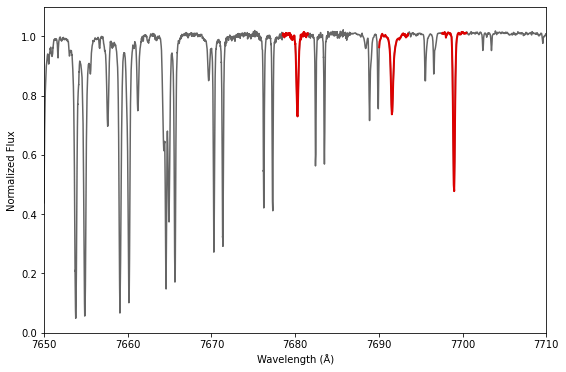
Figure 1: An excerpt from the spectrum of HD 209458 in the range of the red edge of the telluric O₂ A band (seen here as repeating doublets across the spectrum decreasing in depth from left to right). Highlighted in red are three lines of Si, Mg, and K (from left to right), which were used in our analysis. While the left end of the Mg line (center) overlaps with one of the telluric features, this blending is easily ignored by measuring the equivalent width of a model line profile.

4.3 LTE Analysis

Our abundance analysis follows the methods of Kolecki et al. (2021), using equivalent widths with abfind in PyMOOGi (Adamow, 2017) to derive elemental abundances. Some changes were made, as outlined in this section.

4.3.1 Stellar Parameters

The Kolecki et al. (2021) parameter fitting is changed, with the addition of UBVRI photometry compiled by SIMBAD to the previously used Gaia, 2MASS, and WISE data (Gaia Collaboration et al., 2018; Skrutskie et al., 2006; Wright et al., 2010, respectively). Additionally, we took a different approach to sampling stellar parameters, calculating a grid of reduced $\chi^{2}$ statistics containing each point on an isochrone, from which we derive a probability distribution to directly sample T_eff  and log(g) from. This method produces similar results at that used previously (with differences of roughly 1-sigma or less), but allows for a more robust calculation of the uncertainties.

Also, in the case of non-convergence of microturbulence, rather than setting to 1.5 km/s, we chose to set the value to the point on the microturbulence grid that minimized the magnitude of the slope of the correlation with equivalent width.

4.3.2 Uncertainty Analysis

The uncertainty of abundance measurements is calculated as a quadrature sum of the following sources of error: line-to-line scatter of best fit abundance, and the change of abundance from perturbation of the stellar parameters (T_eff, log(g), $\xi$, [Fe/H]) each by 1-$\sigma$. We iterated this calculation to account for the coupled nature of the uncertainties of abundances and stellar parameters. This coupling comes from the fact that the stellar parameters are sampled from isochrones, which vary with metallicity. Thus, a higher uncertainty on [Fe/H] creates a wider distribution of available T_eff and log(g) values to sample from.

Our updated method differs from the previous method (Kolecki et al., 2021; Epstein et al., 2010). This is because the equilibrium conditions (described in Section 6.1 of Kolecki et al., 2021) are not always met. For example, in this particular work, only 8 stars out of 17 analyzed meet all the conditions to within $2\sigma$. For these particular stars, the two methods produce comparable uncertainties. Therefore, the new uncertainty analysis method builds on our old method and remains valid even in the case of stellar disequilibrium.

Note that in the cases of nitrogen and sodium, additional error terms were introduced into the quadrature sum after NLTE corrections were applied (see Sections 4.4.2 and 4.4.5.)

Finally, uncertainties of numerical abundance ratios were calculated according to the formula for combining multiplied uncertainties

$$\sigma_{\textrm{X}/\textrm{Y}}=\frac{\textrm{X}}{\textrm{Y}}*\sqrt{(\frac{\Delta\textrm{X}}{\textrm{X}})^{2}+(\frac{\Delta\textrm{Y}}{\textrm{Y}})^{2}}$$

where $\Delta\textrm{X}$ is the change in numerical abundance by perturbing log($\epsilon_{\textrm{X}}$) by its uncertainty.

4.4 NLTE corrections

Calculating abundances in LTE sacrifices accuracy for a significant decrease in computational complexity, as many of the simplifying approximations made in the LTE assumption are imperfect representations of the happenings in a stellar interior (Asplund, 2005).

These NLTE corrections can be important for interpreting and predicting planet formation pathways. For example, Brewer et al. (2016)’s LTE analysis of 55 Cancri, presented in Brewer & Fischer (2016), derives a C/O abundance ratio of 0.53. However, Teske et al. (2013) perform a similar LTE analysis, but with NLTE corrections applied, and derive a C/O ratio of 0.78. Brewer et al. (2016) actually mention the tendency of LTE to overestimate oxygen abundances derived from the O I triplet, which is used in both this work and Brewer et al. (2016), which would thus underestimate C/O. However, they do not apply any corrections for these effects. The resultant discrepancy is significant beyond the error bars, and also has implications for the composition of 55 Cnc e, as Moriarty et al. (2014) define the threshold for carbon-rich exoplanet formation at C/O = 0.65.

Several previous papers included calculated abundances with NLTE radiative transfer code (e.g. MULTI3D, Leenaarts & Carlsson, 2009) for certain sets of stellar parameters. We can thus use these results to improve the accuracy of our analysis. These papers have published values of NLTE corrections, which are the differences in abundances between their NLTE analysis and reference LTE analysis. Adding these differences into our LTE abundances allows us to account for the effects of NLTE without performing the intense calculations usually associated with this. Our NLTE corrections are compiled from a variety of literature sources as listed below. In the event that multiple references for the same corrections were found, we took the most recent available to account for advancements in atomic and atmospheric modelling, as well as in radiative transfer codes.

4.4.1 Carbon And Oxygen

For carbon and oxygen, we interpolated the grid of corrections provided by Amarsi et al. (2019), which covers the extent of the parameter space of our sample. The magnitude of the carbon corrections was $<$ 0.05 dex for all stars. However, the oxygen corrections were more significant, having an average value of roughly -0.2 dex. In the extreme case of the relatively hot, metal-rich sub-giant HD 149026, the oxygen correction reaches a value of -0.33 dex.

4.4.2 Nitrogen

For nitrogen, we used the temperature-dependent NLTE corrections of Takeda & Honda (2005) by performing a linear regression on their data. This introduced an error of 0.015 dex from the scatter of the data points around the best fit line, which was added in quadrature to the uncertainty from Section 4.3.2.

4.4.3 Sulfur

For sulfur, we interpolated the grid of Korotin et al. (2017). Because the sulfur grid was only calculated for log(g) = 4.0, we attempted to extrapolate values for higher surface gravities. Due to the high excitation potential of the sulfur lines used, we did this by looking at the general trend of the correction vs. log(g) for high-excitation lines.

As shown in Figure 2, the corrections show a relatively linear trend towards zero as surface gravity increases in the example case of the O I triplet. The physical reasoning for this is as follows. For computational simplicity, the LTE assumption considers all excitations of electrons to be the result of collisions between atoms (local effects). This neglects the contribution of excited electrons caused by incoming radiation from deeper in the star (non-local effects).

This is a largely fair assumption at high pressures (i.e. higher surface gravities), where high pressure implies higher density of particles. This increased density minimizes the mean free path of photons, reducing the impact of non-local radiation. On the other hand, as pressure is lowered and mean free path increases, photon excitation plays a larger role as more and more photons are able to reach the atoms, causing increasing deviations from the LTE assumption at lower surface gravities.

This trend allows for the assumption that at sufficiently high surface gravities, the magnitude of all NLTE corrections approaches zero. We chose to set this critical log(g) value to be 5.5, based on the extrapolations shown in Figure 2. To use this point to get sulfur corrections at higher surface gravities and given temperature, we linearly interpolated NLTE corrections along the line which connects the value at log(g) = 4.0 to the point at log(g) = 5.5, where corrections are set to be 0.

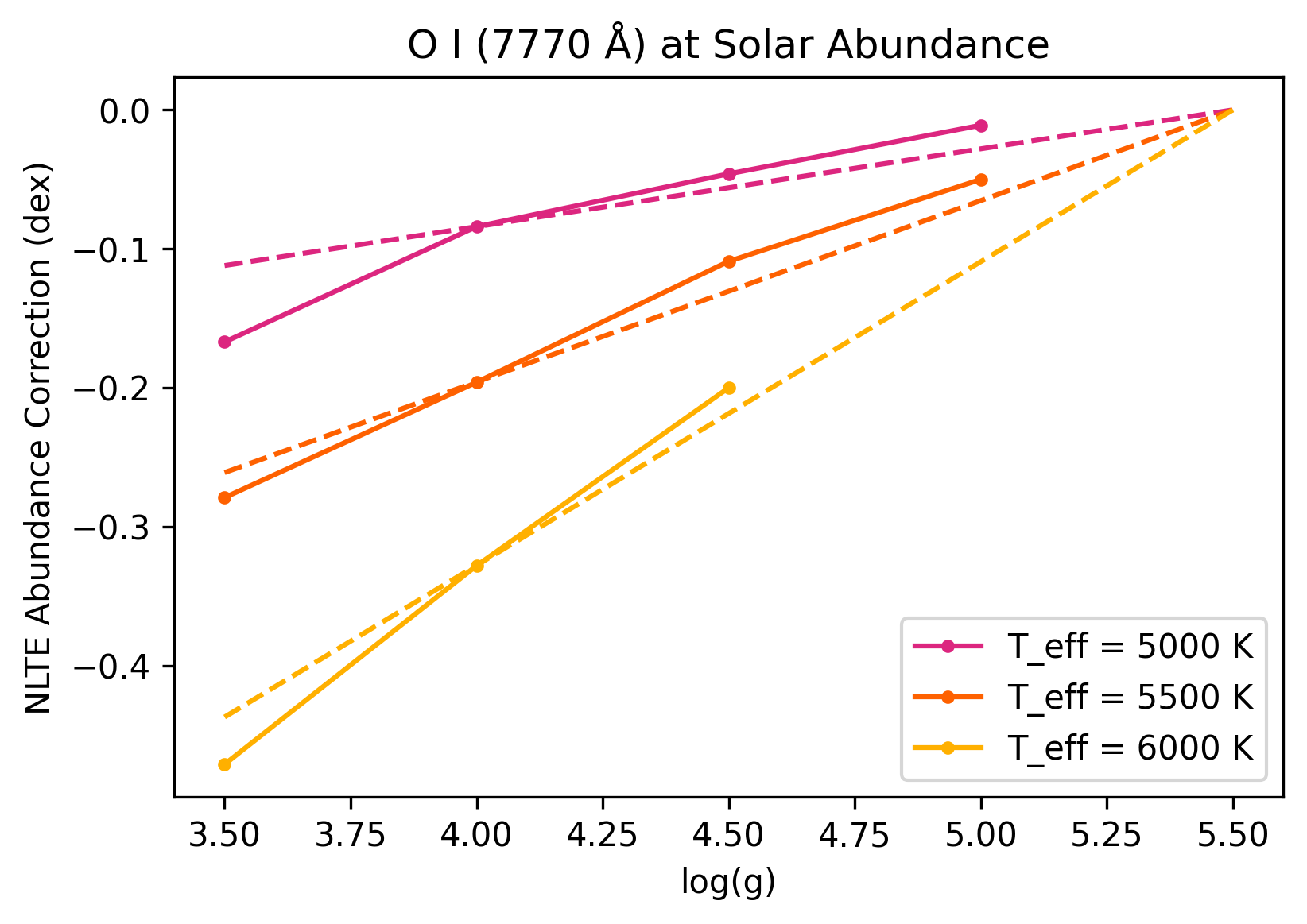
Figure 2: Surface gravity plotted against the magnitude of NLTE corrections for the O I triplet calculated by Amarsi et al. (2019). The dashed lines represent an application of our extrapolation method used for sulfur corrections to those of oxygen. The linear extrapolation from log(g) = 4.0 to 5.5 at each temperature is represented by the dashed line, in which the corrections at 5.5 are assumed to be equal to zero. The deviation of the true corrections from our approximation is minimal, $\lesssim$ 0.03 dex in the relevant parameter space.

These corrections served to lower the sulfur abundance by $<$ 0.1 dex in the case of the 6757Å  and 8694Å  multiplets. However, the 9212Å  multiplet is far more significantly affected. WASP-127 is the star with the most significant sulfur corrections. For this star, the NLTE correction for the 9212Å  line is roughly -0.3 dex with respect to LTE.

4.4.4 Magnesium and Silicon

For these elements, we used the Spectrum Tools utility (http://nlte.mpia.de, M. Kovalev et al., 2018), which interpolates Mg corrections as calculated for Bergemann et al. (2017) and Si corrections as calculated for Bergemann et al. (2013). These corrections were found to minimally change their respective abundances, lowering them by a maximum of 0.01 dex for our chosen lines.

4.4.5 Sodium

For sodium, we adjusted our LTE abundances according to the contour plot presented in Figure 4 of Lind et al. (2011). Given our choice of lines, the correction lowers the Na abundance by 0.1 dex for each of our stars. We introduced an uncertainty of $\pm 0.025$ dex to account for potential small fluctuations in the correction within the precision of the contour plot. This term was added into the uncertainty from Section 4.3.2.

4.4.6 Potassium

For potassium, we used an interpolator hosted at http://www2.nao.ac.jp/~takedayi/potassium_nonlte/ (Takeda et al., 2002). For both WASP-17 and HD 149026, the NLTE correction lowers the LTE potassium abundance by more than 0.5 dex.

5 Results and Discussion

Table 3 shows the stellar parameters of our target stars, while Table 5 displays the results of our abundance analysis. Our iron abundances were taken as the average of the abundances derived from Fe I and Fe II lines. To confirm the validity of the comparison to solar abundances, we analyzed a solar spectrum from FEROS and found that our analysis was in agreement with values from Asplund et al. (2021). The value of the NLTE corrections applied to the initial LTE abundance, $\textrm{log}(\epsilon_{\textrm{x}})_{\textrm{LTE}}$, are shown in Table 6. In Table 6, we display relevant numerical abundance ratios as mentioned in Sections 2.2 and 2.3.

The empty entries in Table 5 are the result of non-detection of atomic lines of the given species. This is due to the weakness of the lines combined with an SNR which makes them unresolvable from noise.

Table 3: Stellar Parameters (units defined as follows: T_eff in K, log(g) in [cm/s²], $\xi$ in km/s, [Fe/H] in dex relative to solar)

Star Name	Teff	log(g)	$\xi$	[Fe/H]
18 Eridani	5097 $\pm$50	4.58 $\pm$0.02	0.79 $\pm$0.24	-0.05 $\pm$0.10
18 Indi	4682 $\pm$40	4.60 $\pm$0.02	0.50 $\pm$0.24	-0.12 $\pm$0.07
55 Cancri	5308 $\pm$40	4.46 $\pm$0.03	1.14 $\pm$0.18	0.30 $\pm$0.06
HAT-P-1	5812 $\pm$190	4.26 $\pm$0.09	1.16 $\pm$0.07	0.01 $\pm$0.11
HAT-P-26	5289 $\pm$80	4.52 $\pm$0.02	0.50 $\pm$0.27	0.02 $\pm$0.10
HD 80606	5547 $\pm$40	4.37 $\pm$0.04	1.51 $\pm$0.24	0.19 $\pm$0.09
HD 149026	6029 $\pm$20	4.20 $\pm$0.02	1.04 $\pm$0.11	0.31 $\pm$0.09
HD 189733	5099 $\pm$30	4.56 $\pm$0.02	1.52 $\pm$0.18	-0.12 $\pm$0.08
HD 209458	6031 $\pm$20	4.31 $\pm$0.02	1.12 $\pm$0.13	-0.01 $\pm$0.06
Kepler-51	5577 $\pm$40	4.46 $\pm$0.02	1.63 $\pm$0.15	-0.29 $\pm$0.07
TOI 193	5410 $\pm$50	4.42 $\pm$0.03	1.71 $\pm$0.15	0.02 $\pm$0.08
TOI 421	5324 $\pm$60	4.52 $\pm$0.02	0.50 $\pm$0.35	-0.03 $\pm$0.08
WASP-17	6157 $\pm$150	4.02 $\pm$0.05	1.53 $\pm$0.17	-0.30 $\pm$0.11
WASP-52	5121 $\pm$60	4.55 $\pm$0.03	1.25 $\pm$0.26	0.08 $\pm$0.09
WASP-63	5512 $\pm$80	3.94 $\pm$0.04	1.53 $\pm$0.12	-0.01 $\pm$0.15
WASP-77A	5660 $\pm$60	4.49 $\pm$0.03	1.78 $\pm$0.15	-0.15 $\pm$0.06
WASP-127	5949 $\pm$60	4.24 $\pm$0.02	1.57 $\pm$0.10	-0.35 $\pm$0.05

Note. — $log(\epsilon_{Fe})_{\odot}=7.46$ (Asplund et al., 2021)

Table 5: Abundance data in log($\epsilon_{X}$) for target stars

Star Name	Fe	C	N	O	S	Mg	Si	Na	K
Sun	7.46 $\pm$0.04	8.46 $\pm$0.04	7.83 $\pm$0.07	8.69 $\pm$0.04	7.12 $\pm$0.03	7.55 $\pm$0.03	7.51 $\pm$0.03	6.22 $\pm$0.03	5.07 $\pm$0.03
18 Eridani	7.41 $\pm$0.10	8.41 $\pm$0.05	…	8.75 $\pm$0.08	6.96 $\pm$0.07	7.48 $\pm$0.04	7.49 $\pm$0.04	6.26 $\pm$0.05	5.01 $\pm$0.05
18 Indi	7.34 $\pm$0.07	8.27 $\pm$0.05	…	8.58 $\pm$0.04	6.86 $\pm$0.06	7.52 $\pm$0.07	7.57 $\pm$0.06	6.02 $\pm$0.09	4.91 $\pm$0.05
55 Cancri	7.76 $\pm$0.06	8.80 $\pm$0.01	8.08 $\pm$0.08	8.88 $\pm$0.04	7.56 $\pm$0.05	8.15 $\pm$0.05	8.04 $\pm$0.06	6.83 $\pm$0.05	5.28 $\pm$0.02
HAT-P-1	7.47 $\pm$0.11	8.49 $\pm$0.09	8.05 $\pm$0.09	8.78 $\pm$0.07	7.08 $\pm$0.10	7.67 $\pm$0.05	7.70 $\pm$0.04	6.33 $\pm$0.08	5.07 $\pm$0.08
HAT-P-26	7.48 $\pm$0.10	8.51 $\pm$0.03	…	8.56 $\pm$0.06	7.27 $\pm$0.05	7.88 $\pm$0.07	7.75 $\pm$0.04	6.43 $\pm$0.12	5.24 $\pm$0.04
HD 80606	7.65 $\pm$0.09	8.72 $\pm$0.07	…	8.82 $\pm$0.03	7.39 $\pm$0.04	8.00 $\pm$0.06	7.91 $\pm$0.07	6.80 $\pm$0.06	5.13 $\pm$0.06
HD 149026	7.77 $\pm$0.09	8.70 $\pm$0.07	…	8.83 $\pm$0.02	7.26 $\pm$0.09	7.96 $\pm$0.12	7.88 $\pm$0.07	6.44 $\pm$0.06	5.12 $\pm$0.02
HD 189733	7.34 $\pm$0.08	8.56 $\pm$0.09	7.62 $\pm$0.03	8.76 $\pm$0.05	6.82 $\pm$0.08	7.42 $\pm$0.04	7.48 $\pm$0.04	6.21 $\pm$0.07	5.00 $\pm$0.02
HD 209458	7.45 $\pm$0.06	8.32 $\pm$0.03	7.83 $\pm$0.06	8.64 $\pm$0.02	7.09 $\pm$0.05	7.66 $\pm$0.08	7.57 $\pm$0.05	6.10 $\pm$0.05	4.94 $\pm$0.03
Kepler-51	7.17 $\pm$0.07	8.23 $\pm$0.23	…	8.68 $\pm$0.04	…	7.40 $\pm$0.03	7.36 $\pm$0.06	5.97 $\pm$0.05	4.84 $\pm$0.04
TOI 193	7.48 $\pm$0.08	8.66 $\pm$0.08	…	8.88 $\pm$0.06	7.62 $\pm$0.08	7.92 $\pm$0.07	7.75 $\pm$0.04	6.45 $\pm$0.04	4.94 $\pm$0.04
TOI 421	7.43 $\pm$0.08	8.41 $\pm$0.05	7.91 $\pm$0.06	8.62 $\pm$0.08	7.47 $\pm$0.05	7.70 $\pm$0.07	7.72 $\pm$0.12	6.12 $\pm$0.04	5.05 $\pm$0.05
WASP-17	7.16 $\pm$0.11	8.32 $\pm$0.09	7.91 $\pm$0.11	8.83 $\pm$0.09	6.69 $\pm$0.10	7.24 $\pm$0.09	7.44 $\pm$0.10	6.34 $\pm$0.25	4.73 $\pm$0.14
WASP-52	7.54 $\pm$0.09	8.53 $\pm$0.07	…	8.93 $\pm$0.15	7.31 $\pm$0.19	7.67 $\pm$0.10	7.84 $\pm$0.05	6.46 $\pm$0.10	5.16 $\pm$0.07
WASP-63	7.45 $\pm$0.15	8.60 $\pm$0.12	7.64 $\pm$0.07	8.82 $\pm$0.09	7.18 $\pm$0.06	7.78 $\pm$0.10	7.71 $\pm$0.07	6.30 $\pm$0.10	5.04 $\pm$0.13
WASP-77A	7.31 $\pm$0.06	8.42 $\pm$0.04	7.86 $\pm$0.08	8.65 $\pm$0.04	6.88 $\pm$0.03	7.53 $\pm$0.07	7.51 $\pm$0.07	6.12 $\pm$0.06	4.96 $\pm$0.04
WASP-127	7.11 $\pm$0.05	8.12 $\pm$0.07	7.83 $\pm$0.07	8.44 $\pm$0.04	6.64 $\pm$0.08	7.42 $\pm$0.05	7.41 $\pm$0.04	5.95 $\pm$0.03	4.80 $\pm$0.03

Note. — Solar abundances are for reference and are sourced from Asplund et al. (2021). Null entries in the table are a result of complete non-detection of atomic lines of a given species for a given star.

Table 6: NLTE corrections, $\delta$, such that $\textrm{log}(\epsilon_{\textrm{x}})_{\textrm{LTE}}+\delta=\textrm{log}(\epsilon_{\textrm{x}})_{\textrm{Final}}$

Star Name	Fe	C	N	O	S	Mg	Si	Na	K
18 Eridani	0.00	-0.01	…	-0.06	-0.37	-0.01	0.00	-0.10	-0.06
18 Indi	0.00	-0.01	…	-0.04	-0.07	-0.01	0.00	-0.10	-0.01
55 Cancri	0.00	0.00	-0.03	-0.10	-0.02	0.00	0.00	-0.10	-0.16
HAT-P-1	0.00	-0.03	-0.07	-0.24	0.00	0.00	-0.01	-0.10	-0.33
HAT-P-26	0.00	0.00	…	-0.09	0.00	-0.00	0.00	-0.10	-0.15
HD 80606	0.00	-0.01	…	-0.12	-0.02	0.00	-0.01	-0.10	-0.19
HD 149026	0.00	0.00	…	-0.33	-0.10	0.00	-0.01	-0.10	-0.55
HD 189733	0.00	-0.01	-0.02	-0.03	-0.06	-0.01	-0.01	-0.10	-0.14
HD 209458	0.00	-0.02	-0.09	-0.27	-0.09	-0.01	0.00	-0.10	-0.50
Kepler-51	0.00	-0.02	…	-0.09	…	-0.01	0.00	-0.10	-0.15
TOI 193	0.00	0.00	…	-0.08	-0.02	-0.01	0.00	-0.10	-0.13
TOI 421	0.00	-0.01	-0.03	-0.10	-0.02	-0.01	0.00	-0.10	-0.14
WASP-17	0.00	-0.03	-0.10	-0.34	-0.06	-0.01	-0.01	-0.10	-0.62
WASP-52	0.00	-0.01	…	-0.05	-0.07	-0.01	0.00	-0.10	-0.11
WASP-63	0.00	-0.02	-0.05	-0.20	-0.03	-0.01	-0.01	-0.10	-0.27
WASP-77A	0.00	0.00	-0.07	-0.10	-0.08	0.00	0.00	-0.10	-0.27
WASP-127	0.00	-0.02	-0.08	-0.20	-0.16	-0.01	-0.01	-0.10	-0.40

Table 6: Stellar Abundance Ratios

Star Name	C/O	N/O	C/N	S/N	Mg/Si
Sun	0.59 $\pm$0.08	0.14 $\pm$0.03	4.27 $\pm$0.85	0.19 $\pm$0.04	1.10 $\pm$0.11
18 Eridani	0.46 $\pm$0.11	…	…	…	0.98 $\pm$0.13
18 Indi	0.49 $\pm$0.08	…	…	…	0.89 $\pm$0.20
55 Cancri	0.83 $\pm$0.08	0.16 $\pm$0.04	5.25 $\pm$1.07	0.30 $\pm$0.07	1.29 $\pm$0.25
HAT-P-1	0.51 $\pm$0.17	0.19 $\pm$0.06	2.75 $\pm$0.85	0.11 $\pm$0.03	0.93 $\pm$0.13
HAT-P-26	0.89 $\pm$0.15	…	…	…	1.35 $\pm$0.27
HD 80606	0.79 $\pm$0.15	…	…	…	1.23 $\pm$0.28
HD 149026	0.74 $\pm$0.13	…	…	…	1.20 $\pm$0.44
HD 189733	0.63 $\pm$0.16	0.07 $\pm$0.01	8.71 $\pm$2.1	0.16 $\pm$0.03	0.87 $\pm$0.12
HD 209458	0.48 $\pm$0.04	0.15 $\pm$0.02	3.09 $\pm$0.51	0.18 $\pm$0.03	1.23 $\pm$0.42
Kepler-51	0.35 $\pm$0.25	…	…	…	1.10 $\pm$0.18
TOI 193	0.60 $\pm$0.15	…	…	…	1.48 $\pm$0.30
TOI 421	0.62 $\pm$0.15	0.19 $\pm$0.05	3.16 $\pm$0.61	0.36 $\pm$0.07	0.95 $\pm$0.34
WASP-17	0.31 $\pm$0.10	0.12 $\pm$0.04	2.57 $\pm$0.95	0.06 $\pm$0.02	0.63 $\pm$0.22
WASP-52	0.40 $\pm$0.18	…	…	…	0.68 $\pm$0.19
WASP-63	0.60 $\pm$0.24	0.07 $\pm$0.02	9.12 $\pm$3.31	0.35 $\pm$0.08	1.17 $\pm$0.34
WASP-77A	0.59 $\pm$0.08	0.16 $\pm$0.04	3.63 $\pm$0.81	0.10 $\pm$0.02	1.05 $\pm$0.26
WASP-127	0.48 $\pm$0.10	0.25 $\pm$0.05	1.95 $\pm$0.48	0.06 $\pm$0.02	1.02 $\pm$0.16

5.1 Literature Comparison

We find good agreement among the literature on stellar parameter values (see Table 10 and Figure 3). Our values are broadly consistent with previously published sources. More discussion can be found in Section 5.2. Below, we discuss some targets in more detail.

5.1.1 HD 189733

The star that shows the largest discrepancy with Brewer’s measurements, HD 189733 ($\rm{[Fe/H]}_{This~{}work}-\rm{[Fe/H]}_{SPOCS}=-0.18~{}\textrm{dex}$), has been measured by other works to have a metallicity consistent with our measurement. Past results include Montes et al. (2018, $\rm{[Fe/H]}=-0.10$) and Sousa et al. (2018, $\rm{[Fe/H]}=-0.04$), both of which fall within $1\sigma$ of the $\rm{[Fe/H]}=-0.12$ derived by this work.

5.1.2 HAT-P-1

The other notable abundance discrepancy is that of the [Fe/H] value of HAT-P-1. Our analysis of CARMENES spectra results in [Fe/H] = 0.01, a value much lower than that of Brewer et al. (2016). We attempted to resolve this discrepancy by analyzing Keck/HIRES data of HAT-P-1 (PI: Asplund 2013-08-16). While this analysis resulted in a higher metallicity than before ([Fe/H] = 0.09), it resulted in an uncharacteristically high sulfur abundance ([S/H] = 0.50). This is in contrast to the abundances of other volatiles in the star, which scaled evenly according to solar metallicity. Furthermore, this higher [Fe/H] was the result of significant ionization disequilibrium, where [Fe I/H] = -0.02 and [Fe II/H] = 0.19.

It should be noted that the literature distribution of the log(g) value of HAT-P-1 is broad, which may account for some of this variation. The results of this work (log(g) = 4.26) align more closely with the results of Brewer et al. (2016) (log(g) = 4.32) when compared to other literature values (e.g. Liu et al., 2014, log(g) = 4.43).

In the end, we have decided to keep the results of the CARMENES spectrum, which were consistent with reasonable expectations of the distribution of abundances of various elements. Furthermore, the large uncertainties on the stellar parameters of HAT-P-1 in this work (larger than those of other mentioned literature sources) allow for consistency within $2\sigma$ despite otherwise significant deviation.

5.1.3 WASP-17

We have also found notable disagreement of T_eff for WASP-17. We derived a T_eff that is significantly lower than that of Anderson et al. (2010), who present the discovery of WASP-17 b, by $\sim$400 K. Conversely, our measurement falls within 60 K of that derived by Gaia DR2 (Gaia Collaboration et al., 2018).

This discrepancy could be due in part to methodology. Gaia effective temperatures are derived from photometry by an algorithm trained on literature catalogs (Andrae et al., 2018). We also used photometry, though in a different capacity, to derive our stellar parameters. In constrast, Anderson et al. (2010) use synthetic spectral fitting as in West et al. (2009), in which H-alpha and H-beta lines are used to derive effective temperature, and the sodium and magnesium Fraunhofer lines are used to derive surface gravity.

Looking further still, WASP-17 has an extremely broad log(g) distribution, significantly wider than that of HAT-P-1. This suggests that something is off when it comes to getting its stellar parameters, although it is difficult to say for certain what the cause is of this. Spectroscopic surface gravities range from log(g) = 4.14 (Torres et al., 2012) to log(g) = 4.83 (Delgado Mena et al., 2015).

Comparing our results with Gaia again results in fair agreement, as the RV template log(g) = 4.0 for WASP-17. This implies that, albeit on an extremely coarse grid (choosing between logg = 3.5, 4.0, 4.5, 5.0), Gaia’s best spectral fit for the purposes of RV retrieval was a logg of 4.0, which matches up with this work’s value of 4.02.

5.2 Effects of Analysis Processes on Abundances

As is visible in Figure 3 and Table 10, we found our stellar parameters T_eff and log(g) agree well with those of Brewer et al. (2016), but our metallicities are systematically lower by 0.08 dex. This could not be explained by differences in the stellar parameters T_eff and log(g), which were minimal by comparison. It also could not be rectified by a simple reanalysis of the sample, which we had hoped would rectify effects of any potential poorly measured line features affecting our results. Thus, we searched the literature for a possible explanation for this discrepancy.

In general, we found that there can be significant differences in abundance measurements, up to 0.05-0.1 dex (Hinkel et al., 2016), due to a number of factors. These factors include, but are not limited to: choice of radiative transfer code (e.g. MOOG for this work, SME (Piskunov & Valenti, 2017) for Brewer et al. (2016)), choice of model atmosphere grid (e.g. Mészáros et al. (2012) for this work, Castelli & Kurucz (2004) for Brewer et al. (2016)), and choice of line list source (e.g. NIST for this work, VALD for Brewer et al. (2016)). See Hinkel et al. (2016); Jofré et al. (2017); Blanco-Cuaresma (2019), and references therein for more detailed discussion of these differences.

Another source of concern was the large scatter of T_eff and logg between this work and the SWEET-Cat catalog (Sousa et al., 2021). Again looking at Table 10, although the mean values of the residuals are approximately 0 (within the error bars), the standard deviation of the residuals of T_eff  is roughly four times the typical error bar on a single T_eff measurement. A similar situation can be seen in the log(g) residuals as well.

Conversely, the residuals of [Fe/H] show a scatter consistent with the measurement error to within 1-2$\sigma$. This implies that our [Fe/H] uncertainties, while larger than others in the literature, are able to account for the systematic errors within the stellar parameters. Therefore, in using the results of this work, it is important to consider the significance of the error bars on our abundance measurements.

While it is not ideal to simply accept these systematic differences, which could significantly affect results, the lack of a single, standardized method for deriving chemical abundances makes it impossible to ensure complete homogeneity of analysis with the literature. Therefore, we have ensured that our abundance analysis process is as rigorous as possible, while acknowledging the potential for minor disagreements, both with and among other rigorously developed pipelines.

With this in mind, we consider our abundances to match up well with the literature, given that more than 80% of our abunadnces fall within the margin for error discussed in Hinkel et al. (2016). The largest deviations are mainly those of nitrogen, an element with extremely difficult-to-measure lines, and of oxygen, which can be explained by our use of NLTE corrections, which lower [O/H] with respect to the values of Brewer et al. (2016). Other outliers are fairly isolated, and may potentially be resolved by performing multiple analyses of varying methodology to form a distribution of results from which a more robust abundance can be determined.

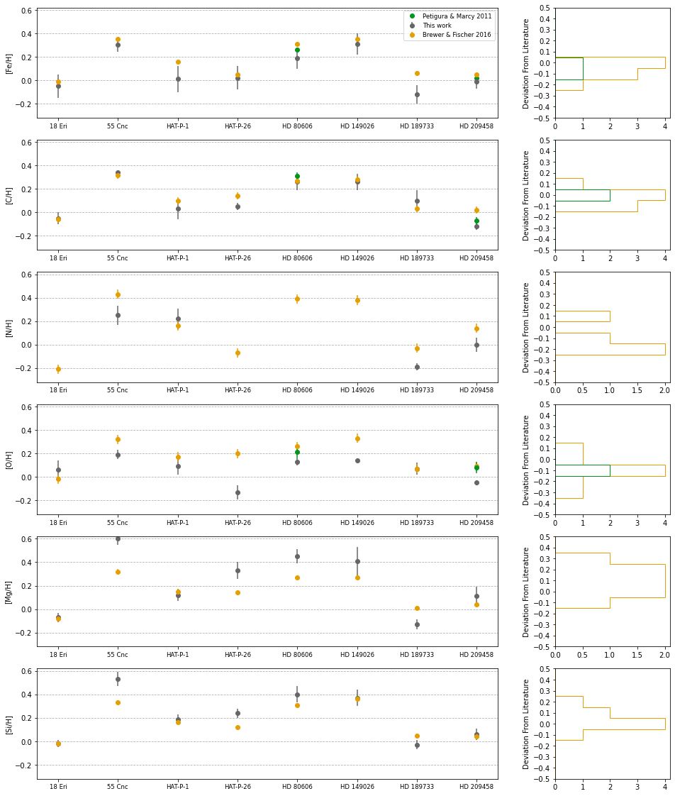
Figure 3: A comparison of abundance values measured by this work (with $1\sigma$ uncertainties) and by Brewer et al. (2016) and Petigura & Marcy (2011). We found that $>80\%$ of our measurements fall within 0.1 dex of the literature, which implies good agreement with previously published values, as outlined in Section 5.2.

5.3 Effects of non-LTE

We also compared our resulting distributions of C/O and Mg/Si with those of Brewer & Fischer (2016). We found good agreement between the average values of our Mg/Si ratios, as shown in Figure 4, and found that NLTE effects change the Mg/Si derived from an LTE analysis negligibly.

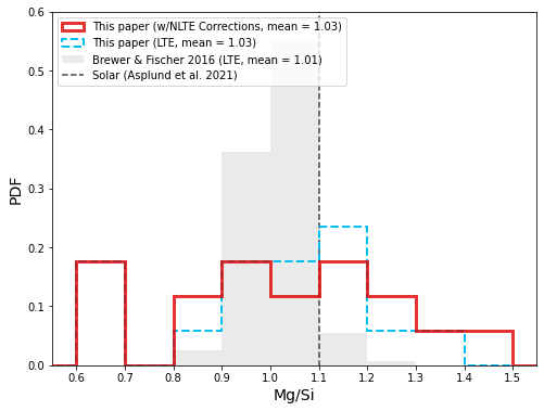
Figure 4: Distribution of Mg/Si ratios of the target stars in LTE and NLTE

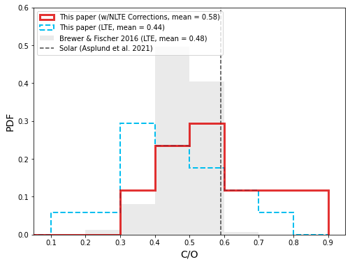
Figure 5: Distribution of C/O ratios of the target stars in LTE and NLTE

In contrast, Figure 5 illustrates the significant NLTE effect on the C/O ratio, as it raises the average of our distribution by 0.14. This is due to the larger decrease in oxygen abundance invoked by NLTE corrections when compared with carbon. Brewer & Fischer (2016) calculate their abundances in LTE without applying NLTE corrections, so we should expect that our mutual LTE C/Os are in agreement, but that our NLTE-corrected C/O ratios are significantly higher. Indeed, we confirm this pattern, also visible in Table 7, which supports the validity of our results.

We discuss that sample selection plays a part in the significant difference in range of values between our two studies in the next section.

5.4 Discrepancies in Literature C/O Distributions

In general, we found disagreement among the literature regarding the distribution of C/O in solar-neighborhood planet hosts, largely centered around oxygen abundances. Some studies (e.g. Petigura & Marcy, 2011) have presented distributions with significantly higher mean values than those of other works (e.g. Nissen, 2013), in spite of both papers’ efforts to compensate for NLTE effects, which should theoretically increase the accuracy of (and thus decrease discrepancy between) both studies.

Petigura & Marcy (2011) perform spectral synthesis of the forbidden 6300Å O I line to derive oxygen abundances, including the blended Ni I feature present in dwarf stars. While this oxygen line is not subject to significant NLTE effects, the blended nickel feature makes an abundance determination via any other method difficult and subject to inaccuracy.

Nissen (2013) uses the O I triplet and applies NLTE corrections to an LTE analysis, the same strategy taken by this work. The C/O distribution of Nissen (2013) shows a similar mean and range in Figure 6 as that of this work (Figure 5), supporting the validity of our analysis. However, the paper goes on to claim that the detection of significant amounts ($\sim 10\%$ of sample stars) of high C/O stars by Petigura & Marcy (2011) is ”spurious,” attributing this to the difficulty in accurately modeling the 6300Å feature with the Ni I blend.

While we do note the significant difference in mean values of the two papers’ distribution (0.63 for Nissen (2013) vs 0.76 for Petigura & Marcy (2011), as shown in Figure 6), both show a modal peak between 0.6 and 0.7. Further, the spread in values of Brewer & Fischer (2016) is significantly lower than those of the other sources shown in the figure. Thus, a number of other factors beyond methodology could be at play. Firstly, small differences in model atmospheres, NLTE corrections, and spectrum synthesis calculation introduces inherent variability as models differ slightly based on things as seemingly minor as the version of the same radiative transfer code being run (e.g. Hinkel et al., 2016; Jofré et al., 2017; Blanco-Cuaresma, 2019, and references therein). This could serve to introduce results between papers for the same star being analyzed.

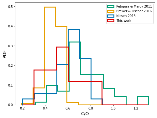
Figure 6: C/O Distribution histograms of this work and various literature sources. The mean values of the distributions are as follows: This work (0.58, LTE w/ NLTE corrections), Brewer & Fischer (0.48, LTE), Nissen (0.63, LTE w/ NLTE corrections), Petigura & Marcy (0.76, LTE [O I]).

Sample size and selection is another factor to consider. We selected 17 planet-hosting targets ($\simeq 0.5\%$ of all such stars discovered at the time of writing), Nissen (2013) selects 33 ($\simeq 1\%$), the analysis of Petigura & Marcy (2011) leaves 72 planet hosts with C/O ratios ($\simeq 2\%$), and Brewer & Fischer (2016) find the C/O ratios of 163 confirmed hosts ($\simeq 4.5\%$). All these studies leave significant gaps in coverage if we are trying to paint a complete picture of all planet-hosting stars. This is especially the case when drawing conclusions about outliers at the extreme high and low ends.

This low sample size also potentially introduces random selection biases into each individual analysis sample. Perhaps Petigura & Marcy (2011) truly did happen to analyze a subset of the whole with higher-than-usual C/Os. This hypothesis is supported by the two stars in common with our sample in Table 7, which have very similar values from both papers.

The opposing hypothesis is that the 6300Å oxygen feature is a bad indicator of abundance even when compensating for blending effects. The best way to answer this question would be to perform a homogeneous analysis of all the stars in all the samples mentioned, which is beyond the scope of this paper.

In general, however, it seems we should expect a C/O distribution of a large sample of planet hosts, based on either an accurate NLTE analysis of the clean, isolated O I triplet feature, or a joint analysis of the Ni I and [O I] blend, to peak around 0.6 and decrease in either direction in a roughly Gaussian fashion.

Table 7: Central C/O values derived by this work and by literature sources (Petigura & Marcy, 2011; Brewer & Fischer, 2016) The bottom row is the average difference between the reference and this work.

Star Name	This work	P&M 2011	B&F 2016
18 Eridani	0.46$\pm$0.11	…	0.48
55 Cancri	0.83$\pm$0.08	…	0.53
HAT-P-1	0.51$\pm$0.17	…	0.46
HAT-P-26	0.89$\pm$0.15	…	0.46
HD 80606	0.79$\pm$0.15	0.79$\pm$0.11	0.54
HD 149026	0.74$\pm$0.13	…	0.48
HD 189733	0.63$\pm$0.16	…	0.49
HD 209458	0.48$\pm$0.04	0.45$\pm$0.06	0.46
Avg. Deviation	…	-0.01	-0.18

Note. — We did not find any common stars between our sample and that of Nissen (2013)

6 Implications

6.1 Finding Carbon-Rich Worlds

Going back to the case of 55 Cancri e, first mentioned in Section 4.4, this is a prime example where NLTE corrections can have a significant impact on abundance results.

With the results of this paper, we can now begin to more precisely estimate the true stellar C/O of 55 Cancri, as we confirm the results of Teske et al. (2013) (C/O = 0.78), deriving a similarly high C/O ratio in this work of 0.83. Thus, we can see more clearly that 55 Cancri e is likely a carbon-dominated planet, given that this is well above the Moriarty et al. (2014) threshold of C/O = 0.65 for short-period carbon-rich planet formation.

This strengthens the case behind the ”diamond planet” model of its interior as discussed in Madhusudhan et al. (2012), where it is shown that mass and radius constraints allow for a planetary composition of $>67\%$ pure carbon, in the form of graphite near the surface, and as diamond as the pressure increases below the surface. This has significant implications as to the potential variations from a purely Earth-like composition of terrestrial exoplanets.

6.2 Tracking Hot Jupiter Formation

A recent paper by Kawashima & Min (2021) provides planetary C/O and N/O for 16 giant planets based on the spectral atmospheric retrieval program ARCiS (Min et al., 2020). This program uses spectral data to solve for the atmospheric parameters of a planet using disequilibrium chemistry. Five of the planets analyzed by Kawashima & Min (2021) orbit stars analyzed by this work, which allows us to compare our stellar elemental ratios with those computed for the planets.

Using the planetary C/O and N/O ratios, along with C/N (which we calculate for the planets by dividing C/O by N/O), we can use the findings of Turrini et al. (2021) to inform about the formation pathways for these planets.

However, we note the large uncertainties associated with the measurement of X/Y*, visible in Table 8. These are largely the result of the propagation of large fractional uncertainties on planetary abundance ratios (often 50% or higher). We await the science results of JWST for these targets, which should significantly reduce the uncertainties with respect to those presented here.

Unfortunately this means that, given presently available data and its associated uncertainties, we are unable to draw definitive conclusions on specific cases of planetary formation. Instead, we present possible indications of formation scenarios, which can be verified in the future by higher-precision data.

Given the abundance patterns outlined in Section 2.3, we show the possibility that both HD 209458 b and HD 189733 b might have underwent significant migration to get to their present orbits, accreting mostly gas along the way. The higher spread of the X/Y* values of HD 189733 b compared with HD 209458 b may be an indication that HD 189733 b have formed further out from its host star than did HD 209458b. However, we reiterate that the high numerical uncertainties make this far from certain.

HAT-P-1 b, on the other hand, may have formed relatively in situ, close to its star. WASP-17 does not appear to follow either pattern, thus no theories can be posited on its formation based on the data shown here.

Table 8: Elemental ratios as defined by Turrini et al. (2021) (see Section 2.3) for stars analyzed by this paper with planets analyzed in Kawashima & Min (2021). In short, values increasing from left to right in the table imply a solid-enriched giant planet, while decreasing values from left to right in the table imply accretion of mostly gaseous matter. Larger spread of these values is associated with higher levels of migration.

Planet Name	N/O*	C/O*	C/N*
HD 189733 b	2.14 $\pm$1.32	0.75 $\pm$0.41	0.36 $\pm$0.29
HD 209458 b	1.27 $\pm$0.62	1.04 $\pm$0.53	0.85 $\pm$0.52
HAT-P-1 b	0.79 $\pm$0.52	0.80 $\pm$0.69	0.99 $\pm$1.04
HAT-P-26 b	…	0.28 $\pm$0.14	…
WASP-17 b	1.33 $\pm$0.90	1.77 $\pm$0.74	1.34 $\pm$1.03

7 Summary

In this paper, we have presented a homogeneous abundance analysis of 17 planet-hosting targets. These planets will be observed by JWST during its first observing cycle. Therefore, we are motivated by the prospects of chemical characterization of exoplanets, and how the composition of a planet’s host star relates to that of the planet. We present the following as the main conclusions which can be drawn from this work:

• Detailed knowledge of a planet’s formation requires accurate chemical abundances of its host star. We have detailed the importance of C, N, O, Na, Mg, Si, S, K, and Fe to planet formation in Section 2.

• Our abundance analysis produces accurate values for stellar parameters (Table 3), abundances (Table 5), and elemental ratios (Table 6) that compare well with the literature where comparisons can be made (see Section 5.1). These values can thus be used to inform future studies on planetary composition that take into account host star composition as well. Furthermore, the accuracy of these results supports the use of our updated framework in future studies, which will shed further light onto the composition of planet-hosting stars.

• NLTE effects on stellar abundance measurements are of strong importance for probing planet formation (see Section 4.4 and Figure 5). Thus, we have compiled sources of corrections for various elements to inform future abundance analyses. We have demonstrated the importance of these corrections with 55 Cancri, a star for which the true C/O ratio has not been fully agreed upon in the literature (see Section 6.1). NLTE corrections serve to significantly raise the stellar C/O compared to its value calculated in LTE.

• The precision levels of currently published spectroscopic observations of planets are too low to provide definitive conclusions on the formation and migration of specific giant planets. However, we have shown that possible preliminary conclusions can be drawn (see Section 6.2 and Table 8). Further, as new science results are published from JWST and other upcoming infrared spectroscopic missions, we can expect abundance analyses with significantly higher levels of precision, from which more robust conclusions can be drawn.

The targets in this paper are almost entirely gas giant hosts, which is in part due to the SNR requirements for observing planets around FGK stars. Our next paper in this series will focus on M dwarfs, a much larger fraction of which have confirmed planets that are super-Earths or smaller.

Table 9: Line Data

Line Information				Equivalent Width For Given Star (mÅ)
$\lambda$ (Å)	X	E.P.(eV)	log(gf)	18 Eri	18 Ind	55 Cnc	HAT-P-1	HAT-P-26	HD 80606	HD 149026	HD 189733	HD 209458	Kepler-51	TOI 193	TOI 421	WASP-17	WASP-52	WASP-63	WASP-77A	WASP-127
4932.030	C I	7.68	-1.66	…	…	…	…	…	…	61.75	…	…	27.07	…	…	39.72	…	…	…	…
5380.330	C I	7.68	-1.62	…	21.61	…	23.07	12.79	26.69	39.49	10.75	22.03	…	18.24	…	25.95	11.83	35.47	15.67	26.58
6587.620	C I	8.54	-1.00	…	…	…	20.00	…	15.41	32.41	…	18.05	…	9.52	…	…	…	16.89	…	11.42
7111.460	C I	8.64	-1.08	…	…	…	11.87	…	…	19.76	…	…	…	14.40	…	…	…	12.47	10.73	5.58
7113.170	C I	8.65	-0.77	…	…	…	21.70	…	…	59.17	…	29.53	11.64	22.78	9.70	…	9.34	48.98	18.10	16.66
7116.980	C I	8.65	-0.91	…	…	…	21.98	…	…	37.63	9.37	21.80	…	…	…	25.79	…	21.87	…	14.81
8058.620	C I	8.84	-1.18	…	…	…	11.32	…	…	14.48	…	…	…	…	…	…	…	10.68	…	…
8335.140	C I	7.68	-0.42	…	…	15.32	…	…	…	…	…	102.39	37.44	…	…	129.20	42.06	69.73	…	69.04
9061.436	C I	7.48	-0.34	…	…	…	…	…	…	…	53.58	…	…	…	…	…	…	…	…	…
9094.830	C I	7.48	0.14	…	…	…	…	…	…	…	126.05	…	…	…	…	…	…	…	…	…
9111.807	C I	7.48	-0.34	63.13	…	…	185.90	…	…	…	…	…	…	…	…	…	…	…	…	139.94
7468.312	N I	10.34	-0.18	…	…	…	5.46	…	…	…	…	4.94	…	…	1.25	…	…	…	2.48	…
8184.860	N I	10.33	-0.30	…	…	2.30	…	…	…	…	…	…	…	…	…	6.12	…	…	…	…
8188.010	N I	10.33	-0.30	…	…	…	…	…	…	…	18.27	4.11	…	…	…	…	…	…	…	4.20
8216.340	N I	10.34	0.14	…	…	…	…	…	…	…	…	…	…	…	…	16.87	…	3.66	…	…
9392.790	N I	10.69	0.30	…	…	…	…	…	…	…	8.13	…	…	…	…	…	…	…	…	6.29
7771.940	O I	9.15	0.37	30.20	47.66	47.65	89.65	35.81	61.50	117.94	26.84	99.91	60.68	53.57	39.81	145.41	30.91	74.59	60.43	81.62
7774.170	O I	9.15	0.22	25.55	43.88	43.88	80.64	…	60.39	106.87	27.10	84.15	52.89	47.59	27.16	123.76	24.59	69.92	56.99	67.16
7775.390	O I	9.15	0.00	14.63	32.83	32.83	64.54	18.41	41.76	85.22	17.32	68.56	35.40	43.81	25.11	98.74	36.71	56.89	41.62	48.00
4668.560	Na I	2.10	-1.31	89.14	…	93.30	…	…	…	…	…	…	…	…	…	…	…	…	…	…
4978.541	Na I	2.10	-1.22	…	…	…	…	…	…	…	…	…	…	…	…	81.89	…	…	…	…
5682.633	Na I	2.10	-0.71	…	…	238.14	134.20	238.53	…	…	…	…	…	…	…	…	…	128.94	113.56	…
5688.205	Na I	2.10	-0.45	…	298.27	242.90	142.47	187.87	198.98	144.38	200.68	116.58	128.54	223.88	179.75	114.19	251.49	135.83	139.74	101.38
6154.225	Na I	2.10	-1.55	64.89	107.88	92.68	39.61	68.44	83.86	50.04	79.71	30.50	39.88	72.92	44.73	9.24	96.16	66.82	50.08	24.45
6160.747	Na I	2.10	-1.25	99.62	…	…	…	…	…	55.75	…	37.99	48.85	…	68.23	…	…	74.71	61.20	38.69
8194.790	Na I	2.10	-0.46	…	…	…	…	…	…	…	497.28	…	…	…	…	184.86	…	…	…	…
9961.256	Na I	3.62	-0.82	…	65.20	…	…	…	…	…	30.78	…	…	…	…	…	…	…	…	…
4057.505	Mg I	4.35	-0.90	…	…	…	…	…	…	…	…	…	…	…	…	212.59	…	…	…	…
5528.405	Mg I	4.35	-0.50	…	576.95	…	…	602.71	508.13	293.59	…	302.50	436.67	…	…	182.00	512.54	357.16	354.95	284.47
7387.689	Mg I	5.75	-1.00	92.86	207.01	95.97	92.51	155.92	152.73	115.16	91.75	…	83.85	140.90	110.46	…	98.85	124.75	87.51	59.00
7691.553	Mg I	5.75	-0.78	140.66	240.87	112.64	131.53	171.60	200.20	177.98	166.89	114.05	96.96	205.08	167.01	47.01	224.86	…	111.51	89.19
8305.596	Mg I	5.93	-1.32	39.72	…	…	…	…	…	…	…	…	…	…	…	…	…	…	…	…
8736.020	Mg I	5.95	-0.72	…	326.08	159.86	…	223.15	309.13	219.73	235.08	…	…	…	…	…	155.57	167.48	157.52	110.07
8923.569	Mg I	5.39	-1.68	72.47	109.94	66.56	53.96	93.65	…	61.03	76.38	45.61	…	…	…	34.07	84.80	69.69	57.39	48.39
9432.764	Mg I	5.93	-0.92	93.54	…	…	…	…	…	…	…	117.33	…	…	…	…	…	…	…	54.32
5645.613	Si I	4.93	-1.63	…	…	…	…	…	75.92	53.54	…	44.04	41.50	…	…	…	…	…	39.44	…
5665.555	Si I	4.92	-2.04	39.52	76.28	26.59	44.91	53.10	62.70	56.18	43.90	36.94	37.27	65.66	63.33	…	67.62	58.86	52.50	30.64
5684.484	Si I	4.95	-1.42	61.71	…	46.24	…	…	…	…	…	…	…	…	…	…	…	…	…	…
5690.425	Si I	4.93	-1.87	42.78	72.70	31.38	56.24	47.90	65.85	62.29	42.39	44.96	61.31	64.54	…	24.08	61.01	65.92	53.93	54.28
5701.104	Si I	4.93	-2.05	30.73	56.88	…	…	49.88	…	…	33.59	…	27.70	51.40	…	…	48.22	55.36	…	22.33
5708.400	Si I	4.95	-1.47	…	…	…	…	…	…	…	…	…	…	…	…	73.69	…	…	…	…
5772.146	Si I	5.08	-1.75	…	…	37.09	52.47	…	73.90	65.44	…	47.29	43.76	70.45	43.72	28.66	56.42	69.88	52.99	39.08
5797.856	Si I	4.95	-2.05	…	…	…	…	…	…	…	…	…	26.09	…	…	55.27	…	…	…	…
5948.541	Si I	5.08	-1.23	…	129.14	71.89	89.97	105.81	131.18	109.47	99.89	86.65	83.71	100.51	88.95	60.20	106.32	112.52	98.65	83.24
7680.266	Si I	5.86	-0.69	66.46	…	56.47	96.55	89.40	…	102.13	70.29	79.93	…	92.25	…	56.39	95.79	99.49	94.16	70.29
8093.232	Si I	5.86	-1.35	…	…	…	…	…	…	…	…	…	…	…	…	…	…	…	…	28.91
8648.470	Si I	6.21	0.05	116.43	…	121.18	171.65	150.97	189.23	187.29	122.47	144.69	…	…	…	137.25	…	121.21	135.81	111.54
5706.100	S I	7.87	-0.93	…	…	…	…	…	…	…	…	…	94.32	…	…	…	…	…	…	…
6757.150	S I	7.87	-0.35	…	15.71	…	…	…	22.04	…	…	22.13	…	19.57	12.43	33.05	…	…	7.93	14.34
6757.180	S I	7.87	-0.24	…	…	…	…	…	…	39.39	…	…	…	…	…	…	…	…	…	…
8633.120	S I	8.40	-0.06	…	…	…	12.32	…	…	…	…	…	…	…	…	…	…	…	…	…
8655.170	S I	8.40	-0.54	…	…	…	…	2.18	…	…	…	…	…	…	…	…	…	…	…	…
8693.980	S I	7.87	-0.54	…	…	…	…	…	…	…	7.95	12.69	…	…	…	…	8.55	…	6.17	6.52
8694.630	S I	7.86	0.08	…	…	…	32.10	…	…	44.18	…	…	…	…	…	…	…	…	…	…
8694.710	S I	7.87	0.05	6.49	27.44	…	…	…	…	…	5.66	33.11	…	…	…	27.77	…	29.51	…	19.56
9212.860	S I	6.52	0.42	…	…	42.68	…	…	…	171.10	…	…	…	…	…	…	…	…	…	…
9212.863	S I	6.52	0.40	87.86	…	…	…	…	…	…	…	192.76	…	…	…	…	89.40	…	129.39	145.91
9228.090	S I	6.52	0.26	…	…	…	107.35	…	…	…	…	…	…	…	…	…	…	…	…	…
9228.093	S I	6.52	0.25	…	…	…	…	…	…	…	…	…	…	…	…	…	…	…	…	92.26
9237.538	S I	6.52	0.03	…	…	…	…	…	…	…	69.96	125.39	…	…	…	…	…	…	…	96.54
7698.965	K I	0.00	-0.18	251.98	254.14	373.88	166.38	261.72	196.72	169.24	284.97	152.35	165.63	191.34	208.31	133.12	288.37	181.10	191.91	152.55
4007.272	Fe I	2.76	-1.28	114.93	…	…	…	110.23	…	…	…	…	…	…	96.23	68.46	…	…	105.74	…
4009.713	Fe I	2.22	-1.25	…	255.35	…	…	…	…	…	…	…	…	…	…	105.71	…	…	…	…
4017.148	Fe I	3.05	-1.06	…	…	149.76	…	…	…	…	…	…	…	…	…	…	…	…	…	…
4067.271	Fe I	2.56	-1.42	119.24	…	…	…	120.32	…	…	…	…	…	…	…	…	…	…	…	…
4067.978	Fe I	3.21	-0.47	…	…	…	…	…	…	…	…	…	…	…	…	114.53	…	…	…	…
4072.502	Fe I	3.43	-1.44	…	…	…	…	…	…	…	…	…	…	…	…	51.75	…	…	…	…
4073.762	Fe I	3.27	-0.90	…	169.69	…	…	…	…	107.55	…	…	…	…	122.81	74.16	…	…	…	…
4078.353	Fe I	2.61	-1.47	…	…	…	…	…	…	…	…	…	…	…	…	86.11	…	…	…	…
4079.838	Fe I	2.86	-1.36	116.45	166.22	…	…	…	…	89.00	…	89.18	144.79	…	130.95	…	145.58	129.10	106.31	…
4107.488	Fe I	2.83	-0.88	…	187.20	…	…	…	…	…	…	…	…	…	…	94.58	…	142.00	146.44	…
4120.206	Fe I	2.99	-1.27	135.84	…	143.39	…	129.47	…	95.12	…	…	…	133.74	121.49	67.11	130.24	108.64	105.19	…
4121.802	Fe I	2.83	-1.45	123.83	139.01	…	…	106.17	…	110.54	…	82.50	…	…	…	65.43	…	107.53	100.64	…
4136.998	Fe I	3.41	-0.45	147.09	…	…	…	…	…	125.70	…	…	119.03	…	136.56	…	…	119.11	…	…
4157.780	Fe I	3.42	-0.40	…	…	…	…	…	…	133.99	…	…	…	…	…	100.39	…	…	…	…
4175.636	Fe I	2.85	-0.83	…	…	…	…	…	…	…	…	…	…	…	…	97.68	…	…	…	…
4184.891	Fe I	2.83	-0.87	…	188.77	…	…	147.74	…	119.10	…	105.72	137.94	…	136.41	…	…	141.04	135.16	…
4196.209	Fe I	3.40	-0.70	…	…	…	…	…	…	98.04	…	…	…	…	…	…	…	…	…	…
4219.359	Fe I	3.57	-0.00	…	259.32	…	…	…	…	…	…	…	…	…	…	…	…	…	…	…
4222.213	Fe I	2.45	-0.97	…	…	…	…	…	…	146.12	…	145.81	…	…	…	103.62	…	…	…	…
4224.171	Fe I	3.37	-0.51	…	236.43	…	…	…	…	…	…	…	…	…	…	…	…	…	…	…
4266.964	Fe I	2.73	-1.81	…	…	…	…	…	…	…	…	…	…	125.26	…	60.67	…	…	…	…
4267.826	Fe I	3.11	-1.17	…	…	…	…	…	…	…	…	…	…	…	…	80.59	…	…	…	…
4298.036	Fe I	3.05	-1.43	…	…	…	…	…	…	…	…	…	…	…	…	65.17	…	…	…	…
4352.734	Fe I	2.22	-1.29	…	…	…	…	…	…	…	…	…	…	…	…	105.35	…	…	…	…
4388.407	Fe I	3.60	-0.68	…	…	…	…	119.91	…	…	…	…	…	…	…	…	…	…	…	…
4422.568	Fe I	2.85	-1.11	…	…	…	…	…	…	…	…	…	…	…	…	82.99	…	…	…	…
4433.782	Fe I	3.60	-1.27	…	…	…	…	77.91	…	…	…	…	…	…	…	…	…	…	…	…
4442.339	Fe I	2.20	-1.25	…	…	…	…	…	…	…	…	147.93	…	…	…	109.04	…	…	…	…
4443.194	Fe I	2.86	-1.04	…	174.59	…	…	…	…	…	…	…	137.16	…	…	…	…	142.63	135.23	…
4446.832	Fe I	3.69	-1.32	84.17	102.26	95.20	…	…	…	…	…	…	87.80	98.86	87.51	…	…	93.48	76.39	…
4447.717	Fe I	2.22	-1.34	…	…	…	…	…	…	…	…	139.32	…	…	…	110.51	…	…	…	…
4476.018	Fe I	2.85	-0.82	…	287.73	…	…	…	…	…	…	…	…	…	…	…	…	…	…	…
4484.220	Fe I	3.60	-0.86	…	…	…	…	…	…	…	…	…	102.09	…	104.97	75.80	128.74	101.58	…	…
4595.358	Fe I	3.30	-1.76	…	…	…	…	…	…	…	…	…	…	…	…	…	…	121.51	101.64	…
4643.463	Fe I	3.65	-1.15	…	…	…	…	…	…	119.68	…	60.92	75.10	…	…	46.38	…	…	…	…
4647.434	Fe I	2.95	-1.35	…	…	…	…	…	…	…	…	…	120.47	…	…	70.01	…	…	…	…
4736.773	Fe I	3.21	-0.75	…	…	…	…	…	…	…	…	143.63	…	…	…	90.94	…	…	…	…
4786.807	Fe I	3.02	-1.61	…	…	…	…	…	…	…	…	…	…	116.44	…	…	…	…	…	…
4789.651	Fe I	3.55	-0.96	107.97	141.88	…	…	…	…	…	…	…	99.93	112.76	…	…	…	…	…	…
4800.649	Fe I	4.14	-1.03	…	108.89	113.31	…	91.18	102.25	76.34	99.01	…	…	96.17	82.78	…	106.41	93.72	79.11	…
4872.137	Fe I	2.88	-0.57	…	…	…	…	…	…	…	…	…	…	…	…	121.11	…	…	…	…
4878.211	Fe I	2.89	-0.89	…	411.41	…	…	…	…	…	…	…	…	…	…	…	…	…	…	…
4903.310	Fe I	2.88	-0.93	…	262.36	…	…	…	…	…	…	…	…	…	…	100.87	…	…	…	…
4930.315	Fe I	3.96	-1.20	108.30	…	…	…	…	128.39	97.20	…	73.71	92.86	123.25	103.57	42.08	139.86	106.15	104.74	…
4978.603	Fe I	3.98	-0.88	146.89	…	…	…	…	…	…	…	…	…	…	…	69.07	…	…	129.47	…
4985.253	Fe I	3.93	-0.56	…	…	…	…	…	…	…	…	…	…	…	…	…	…	120.35	…	…
5028.126	Fe I	3.57	-1.12	…	…	…	…	…	…	…	…	…	82.09	…	…	…	…	…	…	…
5049.819	Fe I	2.28	-1.35	…	…	…	…	…	…	…	…	120.87	…	…	…	104.42	…	…	…	…
5068.766	Fe I	2.94	-1.04	…	…	…	…	…	…	…	…	…	…	…	…	93.18	…	…	138.99	…
5171.596	Fe I	1.48	-1.79	…	…	…	…	…	…	…	…	…	…	…	…	113.11	…	…	…	…
5191.454	Fe I	3.04	-0.55	…	…	…	…	…	…	…	…	…	…	…	…	130.32	…	…	…	…
5202.336	Fe I	2.18	-1.84	…	268.78	…	…	…	…	…	…	…	…	…	…	…	…	…	…	…
5215.180	Fe I	3.27	-0.87	…	…	…	…	…	…	…	…	…	…	…	…	80.92	…	127.05	…	…
5217.389	Fe I	3.21	-1.16	…	160.38	…	…	139.81	…	106.45	…	92.95	116.85	…	…	67.99	…	134.19	133.01	…
5232.940	Fe I	2.94	-0.06	…	583.58	…	…	…	…	…	…	…	…	…	…	…	…	…	…	…
5242.490	Fe I	3.63	-0.97	114.26	116.82	…	95.67	110.63	101.69	84.63	…	75.05	84.52	112.38	…	67.07	111.34	95.21	92.98	98.68
5253.462	Fe I	3.28	-1.57	…	…	…	…	…	…	…	…	62.78	80.26	…	…	40.72	106.22	89.83	84.18	56.66
5263.306	Fe I	3.27	-0.88	…	…	…	…	…	…	105.45	…	97.24	127.22	…	…	…	…	138.26	…	…
5266.554	Fe I	3.00	-0.39	…	…	…	…	…	…	…	…	…	…	…	…	114.16	…	…	…	…
5281.789	Fe I	3.04	-0.83	…	…	…	…	…	…	…	…	120.32	…	…	…	96.65	…	…	…	…
5283.621	Fe I	3.24	-0.53	…	…	…	…	…	…	…	…	…	…	…	…	…	…	…	…	144.75
5288.526	Fe I	3.69	-1.51	64.01	88.74	73.17	65.98	72.50	80.39	69.63	100.40	53.48	58.09	66.95	…	30.98	…	74.44	60.21	52.61
5302.300	Fe I	3.28	-0.72	…	286.52	…	…	…	…	…	…	138.90	…	…	…	116.98	…	…	…	127.60
5324.178	Fe I	3.21	-0.10	…	…	…	…	…	…	…	…	…	…	…	…	142.67	…	…	…	…
5341.024	Fe I	1.61	-1.95	…	…	…	…	…	…	…	…	…	…	…	…	116.94	…	…	…	…
5365.399	Fe I	3.57	-1.02	…	…	…	87.43	…	…	…	…	…	…	…	90.08	…	…	87.52	…	73.48
5367.465	Fe I	4.42	0.44	…	240.96	…	…	…	…	140.92	…	137.66	…	…	…	99.90	…	…	…	127.12
5369.961	Fe I	4.37	0.54	…	…	…	…	…	…	…	…	…	…	…	…	143.23	…	…	…	…
5379.573	Fe I	3.69	-1.51	74.69	92.71	71.24	65.15	75.48	82.60	68.03	79.51	52.64	…	85.13	…	34.58	84.68	80.91	72.30	43.29
5383.368	Fe I	4.31	0.65	…	33 …	…	…	…	…	…	…	…	…	…	…	119.59	…	…	…	…
5393.167	Fe I	3.24	-0.71	…	…	…	…	…	…	137.60	…	…	…	…	…	113.92	…	…	…	…
5410.909	Fe I	4.47	0.40	…	…	…	…	…	…	…	…	…	…	…	…	122.89	…	…	…	126.52
5412.783	Fe I	4.43	-1.72	37.81	33.61	38.86	…	24.55	…	…	…	…	13.43	30.22	…	…	34.37	23.57	19.18	9.02
5415.198	Fe I	4.39	0.64	…	332.87	…	…	…	…	…	…	…	…	…	…	126.75	…	…	…	…
5429.696	Fe I	0.96	-1.88	…	640.99	…	…	…	…	…	…	…	…	…	…	…	…	…	…	…
5472.708	Fe I	4.21	-1.50	57.35	79.80	60.27	38.30	65.86	77.97	45.89	61.19	…	43.15	76.56	…	14.91	82.82	66.47	48.76	30.47
5525.543	Fe I	4.23	-1.08	69.94	83.49	94.70	…	72.44	82.70	…	75.63	…	50.97	75.43	68.38	…	88.21	64.35	53.78	40.55
5569.618	Fe I	3.42	-0.49	…	360.87	…	…	…	…	…	…	136.34	…	…	…	99.63	…	…	…	117.47
5572.842	Fe I	3.40	-0.28	…	500.82	…	…	…	…	…	…	…	…	…	…	…	…	…	…	…
5586.755	Fe I	3.37	-0.14	…	…	…	…	…	…	…	…	…	…	…	…	119.36	…	…	…	…
5600.224	Fe I	4.26	-1.42	…	…	…	…	…	…	…	…	…	…	…	…	24.90	…	…	…	…
5624.542	Fe I	3.42	-0.76	…	…	…	135.41	…	…	…	…	…	…	…	…	…	…	…	…	125.98
5661.345	Fe I	4.28	-1.76	26.65	50.18	31.82	20.27	34.85	42.75	26.46	…	…	19.04	43.79	…	…	41.86	…	21.21	10.85
5662.516	Fe I	4.18	-0.57	…	…	…	…	…	…	…	…	…	…	…	…	…	…	…	…	74.70
5686.530	Fe I	4.55	-0.45	125.11	…	…	…	…	…	…	…	…	…	…	…	62.22	…	…	…	71.94
5705.464	Fe I	4.30	-1.35	49.65	59.30	41.62	…	50.24	58.22	43.15	51.37	29.85	38.13	60.19	69.53	…	61.17	53.21	43.81	24.61
5753.122	Fe I	4.26	-0.69	…	…	…	78.88	81.56	…	100.54	…	65.01	82.85	…	92.39	…	107.86	88.82	79.55	70.17
5816.373	Fe I	4.55	-0.60	100.44	…	92.40	…	93.62	…	…	…	72.18	84.85	…	…	41.81	131.62	…	103.34	64.59
5855.075	Fe I	4.61	-1.48	31.35	49.11	32.43	25.70	36.54	40.94	31.70	34.63	22.02	26.81	41.16	…	…	38.61	44.34	33.57	17.99
6065.481	Fe I	2.61	-1.53	…	198.39	…	127.52	…	…	127.96	…	…	120.98	…	137.15	89.41	…	146.82	…	103.09
6136.615	Fe I	2.45	-1.40	…	…	…	…	…	…	…	…	…	…	…	…	105.32	…	…	…	…
6137.691	Fe I	2.59	-1.40	…	…	…	…	…	…	128.34	…	120.27	…	…	…	…	…	…	…	124.09
6141.730	Fe I	3.60	-1.46	…	140.70	…	…	…	123.62	…	…	127.44	…	132.14	138.04	…	…	…	134.38	…
6230.722	Fe I	2.56	-1.28	…	…	…	161.20	…	…	…	…	126.16	…	…	…	102.56	…	…	…	142.28
6232.640	Fe I	3.65	-1.22	…	…	…	85.66	104.07	117.82	88.26	…	77.17	92.98	126.77	98.08	50.45	129.62	117.10	103.07	72.33
6246.318	Fe I	3.60	-0.88	…	…	…	104.33	…	…	122.26	…	110.72	…	…	…	69.51	…	137.91	…	109.99
6252.555	Fe I	2.40	-1.69	…	…	…	126.73	…	…	123.51	…	111.30	129.45	…	144.20	90.17	…	…	140.35	114.03
6301.500	Fe I	3.65	-0.72	…	222.93	…	118.53	…	…	120.32	…	…	121.26	…	145.23	76.52	…	…	…	108.21
6336.823	Fe I	3.69	-0.86	…	183.21	…	112.33	…	…	108.46	…	98.75	117.06	…	123.89	68.33	…	132.60	…	97.65
6400.000	Fe I	3.60	-0.29	…	…	…	…	…	…	…	…	…	…	…	…	126.24	…	…	…	…
6408.017	Fe I	3.69	-1.02	…	…	…	88.44	…	…	92.80	…	…	125.52	…	120.48	…	…	…	…	84.68
6411.648	Fe I	3.65	-0.72	…	…	…	126.13	…	…	123.36	…	…	…	…	…	81.65	…	…	…	121.48
6494.980	Fe I	2.40	-1.27	…	…	…	…	…	…	…	…	…	…	…	…	104.32	…	…	…	115.45
6677.985	Fe I	2.69	-1.42	…	…	…	133.98	…	…	127.67	…	115.30	…	…	…	99.22	…	…	…	119.38
6752.707	Fe I	4.64	-1.20	57.27	78.80	…	4 …	36.84	61.11	44.83	…	28.82	41.43	73.59	42.40	…	80.97	64.29	34.32	25.40
6803.999	Fe I	4.65	-1.50	…	…	…	…	…	…	…	…	…	…	…	25.05	…	…	…	…	…
6804.270	Fe I	4.58	-1.81	…	…	…	…	…	…	…	…	…	…	28.89	…	…	…	…	…	…
6837.005	Fe I	4.59	-1.69	18.19	…	…	22.11	21.74	26.49	22.19	19.13	13.73	…	29.86	20.47	…	27.54	23.93	13.99	…
6854.823	Fe I	4.59	-1.93	…	…	…	…	…	…	…	…	…	…	20.70	…	…	…	…	…	…
8327.055	Fe I	2.20	-1.52	…	…	…	…	…	…	…	…	158.13	…	…	…	119.23	…	…	…	144.69
8387.771	Fe I	2.18	-1.49	…	351.23	…	…	…	…	…	…	…	…	…	…	117.33	…	…	…	…
8598.828	Fe I	4.39	-1.09	64.80	81.51	…	53.08	66.11	…	60.62	73.10	45.87	…	…	…	…	…	75.29	72.86	55.77
8688.623	Fe I	2.18	-1.21	…	…	…	…	…	…	…	…	…	…	…	…	143.88	…	…	…	…
4178.854	Fe II	2.58	-2.44	…	…	53.64	…	…	…	…	…	…	88.52	…	81.38	114.92	88.57	125.02	…	…
4491.397	Fe II	2.86	-2.64	…	…	…	…	…	…	112.76	…	…	…	…	60.18	100.49	71.21	76.85	86.18	…
4515.333	Fe II	2.84	-2.36	…	…	…	…	…	…	126.08	…	120.31	115.81	…	89.17	…	…	134.19	108.13	…
4555.887	Fe II	2.83	-2.25	…	…	…	…	…	…	…	…	…	…	…	…	…	75.34	…	…	…
4576.333	Fe II	2.84	-2.92	…	76.85	28.28	…	59.23	…	86.72	…	78.47	59.65	73.84	45.71	…	70.87	89.25	…	…
4583.829	Fe II	2.81	-1.74	…	190.79	138.57	…	…	…	…	…	…	…	…	…	…	132.52	…	…	…
4629.331	Fe II	2.81	-2.26	103.92	125.22	…	…	117.65	…	128.34	109.82	103.78	108.27	120.93	101.77	113.57	122.24	125.42	109.03	…
5316.609	Fe II	3.15	-1.78	126.06	…	81.27	…	132.53	…	…	…	…	…	…	138.39	…	…	…	…	…
7711.720	Fe II	3.90	-2.45	25.80	…	8.22	60.08	19.27	56.95	77.48	27.63	58.79	45.31	40.88	33.48	66.91	47.99	57.19	42.85	47.16

Table 10: Central effective temperature, log(g), and [Fe/H] values derived by this work and by literature sources (Petigura & Marcy, 2011; Brewer & Fischer, 2016; Sousa et al., 2021) The bottom row is the average difference between the reference and this work, with the error term being the standard deviation of the residuals.

	This work			P&M 2011			B&F 2016			Sousa et al. 2021
Star Name	Teff	log(g)	[Fe/H]	Teff	log(g)	[Fe/H]	Teff	log(g)	[Fe/H]	Teff	log(g)	[Fe/H]
18 Eridani	5097$\pm$50	4.58$\pm$0.02	-0.05$\pm$0.10	…	…	…	5065	4.55	-0.01	5053$\pm$46	4.45$\pm$0.10	-0.14$\pm$0.03
55 Cancri	5308$\pm$40	4.46$\pm$0.03	0.30$\pm$0.06	…	…	…	5250	4.36	0.35	5363$\pm$59	4.28$\pm$0.14	0.33$\pm$0.04
HAT-P-1	5812$\pm$190	4.26$\pm$0.09	0.01$\pm$0.11	…	…	…	5964	4.32	0.16	6074$\pm$16	4.41$\pm$0.03	0.20$\pm$0.01
HAT-P-26	5289$\pm$80	4.52$\pm$0.02	0.02$\pm$0.10	…	…	…	5039	4.45	0.05	5001$\pm$61	4.21$\pm$0.15	0.01$\pm$0.04
HD 80606	5547$\pm$40	4.37$\pm$0.04	0.19$\pm$0.09	5573	4.44	0.26	5524	4.31	0.31	5581$\pm$29	4.33$\pm$0.07	0.33 $\pm$0.02
HD 149026	6029$\pm$20	4.20$\pm$0.02	0.31$\pm$0.09	…	…	…	6084	4.24	0.35	6166$\pm$32	4.35$\pm$0.05	0.37$\pm$0.02
HD 189733	5099$\pm$30	4.56$\pm$0.02	-0.12$\pm$0.08	…	…	…	5023	4.51	0.06	4969$\pm$48	4.30$\pm$0.12	-0.08$\pm$0.03
HD 209458	6031$\pm$20	4.31$\pm$0.02	-0.01$\pm$0.06	6099	4.37	0.02	6052	4.34	0.05	6126$\pm$18	4.50$\pm$0.04	0.04$\pm$0.01
Kepler-51	5577$\pm$40	4.46$\pm$0.02	-0.29$\pm$0.07	…	…	…	…	…	…	5673$\pm$60*	4.70$\pm$0.10*	0.05$\pm$0.04*
TOI 421	5324$\pm$60	4.52$\pm$0.02	-0.03$\pm$0.08	…	…	…	…	…	…	5316$\pm$27	4.35$\pm$0.06	-0.03$\pm$0.02
WASP-17	6157$\pm$150	4.02$\pm$0.05	-0.30$\pm$0.11	…	…	…	…	…	…	6793$\pm$52	4.59$\pm$0.04	-0.01$\pm$0.03
WASP-52	5121$\pm$60	4.55$\pm$0.03	0.08$\pm$0.09	…	…	…	…	…	…	5073$\pm$63	4.36$\pm$0.15	0.17$\pm$0.03
WASP-63	5512$\pm$80	3.94$\pm$0.06	-0.01$\pm$0.15	…	…	…	…	…	…	5676$\pm$40	4.12$\pm$0.06	0.26$\pm$0.03
WASP-77A	5660$\pm$80	4.49$\pm$0.03	-0.15$\pm$0.06	…	…	…	…	…	…	5595$\pm$16	4.41$\pm$0.03	0.01$\pm$0.01
WASP-127	5949$\pm$60	4.24$\pm$0.02	-0.35$\pm$0.05	…	…	…	…	…	…	5832$\pm$14	4.31$\pm$0.03	-0.18$\pm$0.01
Avg. Deviation	…	…	…	47$\pm$21	0.07$\pm$0.01	0.05$\pm$0.02	-26$\pm$108	-0.02$\pm$0.05	0.08$\pm$0.05	52$\pm$204	0.01$\pm$0.22	0.08$\pm$0.13

Note. — We did not find any common stars between our sample and that of Nissen (2013)

Note. — Kepler-51’s data in SWEET-Cat was taken from Petigura et al. (2017)

References

- Adamow (2017) Adamow, M. M. 2017, in American Astronomical Society Meeting Abstracts, Vol. 230, American Astronomical Society Meeting Abstracts #230, 216.07
- Amarsi et al. (2019) Amarsi, A. M., Nissen, P. E., & Skúladóttir, Á. 2019, A&A, 630, A104, doi: 10.1051/0004-6361/201936265
- Anderson et al. (2010) Anderson, D. R., Hellier, C., Gillon, M., et al. 2010, ApJ, 709, 159, doi: 10.1088/0004-637X/709/1/159
- Andrae et al. (2018) Andrae, R., Fouesneau, M., Creevey, O., et al. 2018, A&A, 616, A8, doi: 10.1051/0004-6361/201732516
- Asplund (2005) Asplund, M. 2005, ARA&A, 43, 481, doi: 10.1146/annurev.astro.42.053102.134001
- Asplund et al. (2021) Asplund, M., Amarsi, A. M., & Grevesse, N. 2021, A&A, 653, A141, doi: 10.1051/0004-6361/202140445
- Astropy Collaboration et al. (2013) Astropy Collaboration, Robitaille, T. P., Tollerud, E. J., et al. 2013, A&A, 558, A33, doi: 10.1051/0004-6361/201322068
- Astropy Collaboration et al. (2018) Astropy Collaboration, Price-Whelan, A. M., SipHocz, B. M., et al. 2018, aj, 156, 123, doi: 10.3847/1538-3881/aabc4f
- Bergemann et al. (2017) Bergemann, M., Collet, R., Amarsi, A. M., et al. 2017, ApJ, 847, 15, doi: 10.3847/1538-4357/aa88cb
- Bergemann et al. (2013) Bergemann, M., Kudritzki, R.-P., Würl, M., et al. 2013, ApJ, 764, 115, doi: 10.1088/0004-637X/764/2/115
- Blanco-Cuaresma (2019) Blanco-Cuaresma, S. 2019, MNRAS, 486, 2075, doi: 10.1093/mnras/stz549
- Booth et al. (2017) Booth, R. A., Clarke, C. J., Madhusudhan, N., & Ilee, J. D. 2017, MNRAS, 469, 3994, doi: 10.1093/mnras/stx1103
- Brewer & Fischer (2016) Brewer, J. M., & Fischer, D. A. 2016, ApJ, 831, 20, doi: 10.3847/0004-637X/831/1/20
- Brewer et al. (2016) Brewer, J. M., Fischer, D. A., Valenti, J. A., & Piskunov, N. 2016, ApJS, 225, 32
- Brewer et al. (2018) Brewer, J. M., Wang, S., Fischer, D. A., & Foreman-Mackey, D. 2018, ApJ, 867, L3, doi: 10.3847/2041-8213/aae710
- Castelli & Kurucz (2004) Castelli, F., & Kurucz, R. L. 2004, A&A, 419, 725, doi: 10.1051/0004-6361:20040079
- Chen et al. (2020) Chen, G., Casasayas-Barris, N., Pallé, E., et al. 2020, A&A, 635, A171, doi: 10.1051/0004-6361/201936986
- Delgado Mena et al. (2015) Delgado Mena, E., Bertrán de Lis, S., Adibekyan, V. Z., et al. 2015, A&A, 576, A69, doi: 10.1051/0004-6361/201425433
- Epstein et al. (2010) Epstein, C. R., Johnson, J. A., Dong, S., et al. 2010, ApJ, 709, 447, doi: 10.1088/0004-637X/709/1/447
- Espinoza et al. (2017) Espinoza, N., Fortney, J. J., Miguel, Y., Thorngren, D., & Murray-Clay, R. 2017, ApJ, 838, L9, doi: 10.3847/2041-8213/aa65ca
- Fischer & Valenti (2005) Fischer, D. A., & Valenti, J. 2005, ApJ, 622, 1102, doi: 10.1086/428383
- Fogg & Nelson (2007) Fogg, M. J., & Nelson, R. P. 2007, A&A, 461, 1195, doi: 10.1051/0004-6361:20066171
- Gaia Collaboration et al. (2018) Gaia Collaboration, Brown, A. G. A., Vallenari, A., et al. 2018, A&A, 616, A1, doi: 10.1051/0004-6361/201833051
- Gardner et al. (2006) Gardner, J. P., Mather, J. C., Clampin, M., et al. 2006, Space Sci. Rev., 123, 485, doi: 10.1007/s11214-006-8315-7
- Hinkel et al. (2014) Hinkel, N. R., Timmes, F. X., Young, P. A., Pagano, M. D., & Turnbull, M. C. 2014, AJ, 148, 54, doi: 10.1088/0004-6256/148/3/54
- Hinkel et al. (2016) Hinkel, N. R., Young, P. A., Pagano, M. D., et al. 2016, ApJS, 226, 4, doi: 10.3847/0067-0049/226/1/4
- Jofré et al. (2017) Jofré, P., Heiter, U., Worley, C. C., et al. 2017, A&A, 601, A38, doi: 10.1051/0004-6361/201629833
- Kawashima & Min (2021) Kawashima, Y., & Min, M. 2021, arXiv e-prints, arXiv:2110.13443. https://arxiv.org/abs/2110.13443
- Kolecki et al. (2021) Kolecki, J. R., Wang, J., Johnson, J. A., et al. 2021, AJ, 162, 125, doi: 10.3847/1538-3881/ac14bc
- Korotin et al. (2017) Korotin, S., Andrievsky, S., Caffau, E., & Bonifacio, P. 2017, in Astronomical Society of the Pacific Conference Series, Vol. 510, Stars: From Collapse to Collapse, ed. Y. Y. Balega, D. O. Kudryavtsev, I. I. Romanyuk, & I. A. Yakunin, 141
- Kramida et al. (2020) Kramida, A., Yu. Ralchenko, Reader, J., & and NIST ASD Team. 2020, NIST Atomic Spectra Database (ver. 5.8), [Online]. Available: https://physics.nist.gov/asd National Institute of Standards and Technology, Gaithersburg, MD.
- Leenaarts & Carlsson (2009) Leenaarts, J., & Carlsson, M. 2009, in Astronomical Society of the Pacific Conference Series, Vol. 415, The Second Hinode Science Meeting: Beyond Discovery-Toward Understanding, ed. B. Lites, M. Cheung, T. Magara, J. Mariska, & K. Reeves, 87
- Lind et al. (2011) Lind, K., Asplund, M., Barklem, P. S., & Belyaev, A. K. 2011, A&A, 528, A103, doi: 10.1051/0004-6361/201016095
- Liu et al. (2014) Liu, F., Asplund, M., Ramirez, I., Yong, D., & Melendez, J. 2014, MNRAS, 442, L51, doi: 10.1093/mnrasl/slu055
- Lothringer et al. (2021) Lothringer, J. D., Rustamkulov, Z., Sing, D. K., et al. 2021, ApJ, 914, 12, doi: 10.3847/1538-4357/abf8a9
- M. Kovalev et al. (2018) M. Kovalev, S. Brinkmann, M. Bergemann, & MPIA IT-department. 2018, NLTE MPIA web server, [Online]. Available: http://nlte.mpia.de Max Planck Institute for Astronomy, Heidelberg.
- Madhusudhan (2019) Madhusudhan, N. 2019, ARA&A, 57, 617, doi: 10.1146/annurev-astro-081817-051846
- Madhusudhan et al. (2017) Madhusudhan, N., Bitsch, B., Johansen, A., & Eriksson, L. 2017, MNRAS, 469, 4102, doi: 10.1093/mnras/stx1139
- Madhusudhan et al. (2012) Madhusudhan, N., Lee, K. K. M., & Mousis, O. 2012, ApJ, 759, L40, doi: 10.1088/2041-8205/759/2/L40
- Mészáros et al. (2012) Mészáros, S., Allende Prieto, C., Edvardsson, B., et al. 2012, AJ, 144, 120, doi: 10.1088/0004-6256/144/4/120
- Min et al. (2020) Min, M., Ormel, C. W., Chubb, K., Helling, C., & Kawashima, Y. 2020, A&A, 642, A28, doi: 10.1051/0004-6361/201937377
- Montes et al. (2018) Montes, D., González-Peinado, R., Tabernero, H. M., et al. 2018, MNRAS, 479, 1332, doi: 10.1093/mnras/sty1295
- Mordasini et al. (2016) Mordasini, C., van Boekel, R., Mollière, P., Henning, T., & Benneke, B. 2016, ApJ, 832, 41, doi: 10.3847/0004-637X/832/1/41
- Moriarty et al. (2014) Moriarty, J., Madhusudhan, N., & Fischer, D. 2014, ApJ, 787, 81, doi: 10.1088/0004-637X/787/1/81
- Nikolov et al. (2018) Nikolov, N., Sing, D. K., Fortney, J. J., et al. 2018, Nature, 557, 526, doi: 10.1038/s41586-018-0101-7
- Nissen (2013) Nissen, P. E. 2013, A&A, 552, A73, doi: 10.1051/0004-6361/201321234
- Öberg et al. (2011) Öberg, K. I., Murray-Clay, R., & Bergin, E. A. 2011, ApJ, 743, L16, doi: 10.1088/2041-8205/743/1/L16
- Petigura & Marcy (2011) Petigura, E. A., & Marcy, G. W. 2011, ApJ, 735, 41, doi: 10.1088/0004-637X/735/1/41
- Petigura et al. (2017) Petigura, E. A., Howard, A. W., Marcy, G. W., et al. 2017, AJ, 154, 107, doi: 10.3847/1538-3881/aa80de
- Piskunov & Valenti (2017) Piskunov, N., & Valenti, J. A. 2017, A&A, 597, A16, doi: 10.1051/0004-6361/201629124
- Price-Whelan et al. (2018) Price-Whelan, A. M., Sipőcz, B., Günther, H., et al. 2018, The Astronomical Journal, 156, 123
- Savini et al. (2018) Savini, G., Tessenyi, M., Tinetti, G., et al. 2018, in Space Telescopes and Instrumentation 2016: Optical, Infrared, and Millimeter Wave, ed. H. A. MacEwen, G. G. Fazio, M. Lystrup, N. Batalha, N. Siegler, & E. C. Tong, Vol. 9904, International Society for Optics and Photonics (SPIE), 1514 – 1532, doi: 10.1117/12.2233691
- Schulze et al. (2021) Schulze, J. G., Wang, J., Johnson, J. A., et al. 2021, PSJ, 2, 113, doi: 10.3847/PSJ/abcaa8
- Seager & Sasselov (2000) Seager, S., & Sasselov, D. D. 2000, ApJ, 537, 916, doi: 10.1086/309088
- Sedaghati et al. (2016) Sedaghati, E., Boffin, H. M. J., Jeřabková, T., et al. 2016, A&A, 596, A47, doi: 10.1051/0004-6361/201629090
- Shibata et al. (2020) Shibata, S., Helled, R., & Ikoma, M. 2020, A&A, 633, A33, doi: 10.1051/0004-6361/201936700
- Skrutskie et al. (2006) Skrutskie, M. F., Cutri, R. M., Stiening, R., et al. 2006, AJ, 131, 1163, doi: 10.1086/498708
- Sneden (1973) Sneden, C. 1973, ApJ, 184, 839, doi: 10.1086/152374
- Sousa et al. (2018) Sousa, S. G., Adibekyan, V., Delgado-Mena, E., et al. 2018, A&A, 620, A58, doi: 10.1051/0004-6361/201833350
- Sousa et al. (2021) —. 2021, A&A, 656, A53, doi: 10.1051/0004-6361/202141584
- Spalding & Batygin (2017) Spalding, C., & Batygin, K. 2017, AJ, 154, 93, doi: 10.3847/1538-3881/aa8174
- Takeda & Honda (2005) Takeda, Y., & Honda, S. 2005, PASJ, 57, 65, doi: 10.1093/pasj/57.1.65
- Takeda et al. (2002) Takeda, Y., Zhao, G., Chen, Y.-Q., Qiu, H.-M., & Takada-Hidai, M. 2002, PASJ, 54, 275, doi: 10.1093/pasj/54.2.275
- Teske et al. (2013) Teske, J. K., Cunha, K., Schuler, S. C., Griffith, C. A., & Smith, V. V. 2013, ApJ, 778, 132, doi: 10.1088/0004-637X/778/2/132
- Thorngren et al. (2016) Thorngren, D. P., Fortney, J. J., Murray-Clay, R. A., & Lopez, E. D. 2016, ApJ, 831, 64, doi: 10.3847/0004-637X/831/1/64
- Tinetti et al. (2018) Tinetti, G., Drossart, P., Eccleston, P., et al. 2018, Experimental Astronomy, 46, 135, doi: 10.1007/s10686-018-9598-x
- Torres et al. (2012) Torres, G., Fischer, D. A., Sozzetti, A., et al. 2012, ApJ, 757, 161, doi: 10.1088/0004-637X/757/2/161
- Turrini et al. (2021) Turrini, D., Schisano, E., Fonte, S., et al. 2021, ApJ, 909, 40, doi: 10.3847/1538-4357/abd6e5
- Vidal-Madjar et al. (2011) Vidal-Madjar, A., Sing, D. K., Lecavelier Des Etangs, A., et al. 2011, A&A, 527, A110, doi: 10.1051/0004-6361/201015698
- Virtanen et al. (2020) Virtanen, P., Gommers, R., Oliphant, T. E., et al. 2020, Nature Methods, 17, 261, doi: 10.1038/s41592-019-0686-2
- Wang et al. (2018) Wang, H. S., Lineweaver, C. H., & Ireland, T. R. 2018, Icarus, 299, 460, doi: 10.1016/j.icarus.2017.08.024
- Wang & Fischer (2015) Wang, J., & Fischer, D. A. 2015, AJ, 149, 14, doi: 10.1088/0004-6256/149/1/14
- Wang & Dai (2019) Wang, L., & Dai, F. 2019, ApJ, 873, L1, doi: 10.3847/2041-8213/ab0653
- West et al. (2009) West, R. G., Anderson, D. R., Gillon, M., et al. 2009, AJ, 137, 4834, doi: 10.1088/0004-6256/137/6/4834
- Wright et al. (2010) Wright, E. L., Eisenhardt, P. R. M., Mainzer, A. K., et al. 2010, AJ, 140, 1868, doi: 10.1088/0004-6256/140/6/1868