A fully non-perturbative charm-quark tuning
using machine learning

Abstract

We present a relativistic heavy-quark action tuning for the charm sector on ensembles generated by the CLS consortium. We tune a particular 5-parameter action in an entirely non-perturbative and – up to the chosen experimental input – model-independent way using machine learning and the continuum experimental charmonium ground-state masses with various quantum numbers. In the end we are reasonably successful; obtaining a set of simulation parameters that we then verify produces the expected spectrum. In the future, we will use this action for finite-volume calculations of hadron-hadron scattering.

I Introduction

In recent years, studies of hadron-hadron scattering using Lüscher’s finite volume method [1, 2] have become the state of the art for obtaining information about physical scattering amplitudes from Lattice QCD. In the light-quark sector, such studies typically make use of moving frames to maximise the information about scattering amplitudes deduced from a single gauge field ensemble (for examples, please refer to [3]).

For hadrons with heavy charm or bottom quarks, using the Wilson-clover action [4] employed for the light (up, down, and strange) quarks leads to large heavy-quark discretisation effects. These discretisation effects can be understood in the context of the Fermilab approach [5, 6]. While the simplest implementation of such a relativistic heavy quark (RHQ) action used by the Fermilab Lattice and MILC collaborations (see [7, 8]) tunes the kinetic masses of spin-averaged ground states and thereby obtains an excellent description of ground-state mass splittings in the charmonium spectrum [9], large discretisation effects are still present in hadronic dispersion relations [6, 10].

For the study of hadron resonances and bound states with Lüscher’s finite volume method, such an approach was used for heavy-light mesons in [11, 10, 12] and for charmonium in [13]. Due to the non-standard dispersion relation in the Fermilab method with [5, 6] $M_{1}\neq M_{2}\neq M_{4}\dots$, these studies only used rest-frame data, as there is no simple expression for a change of frame from interacting two-hadron energies in moving frames to the center-of-momentum frame consistent with the Fermilab method dispersion relation. In more recent studies of the charmonium spectrum in (coupled-channel) scattering of charmed mesons [14, 15], moving frames were used by only extracting energy differences with regard to close-by non-interacting meson-meson levels and by purely working with the continuum form of the dispersion relations, which minimises the effects from heavy-quark discretisation effects . This introduces a hard-to-quantify systematic uncertainty.

To reduce the uncertainty from heavy-quark discretisation effects in the context of scattering studies, it is therefore desirable to at least tune the dispersion relation to be approximately relativistic with a speed of light $c=1$ (in natural units). In the next section we will describe the lattice gauge field ensembles used in our simulation, introduce the relativistic heavy-quark action used, and describe the methodology for a fully non-perturbative tuning of this action. In Section III we proceed to show the outcome of this tuning procedure, and compare it to the charm simulations with the CLS light-quark action. In Section IV we summarize our results and provide a brief outlook.

II Methodology

II.1 Gauge field ensembles

$\beta$	Name	$L^{3}\times L_{T}$	T-Boundary	$N_{\text{conf}}\times N_{\text{src}}$	$a^{-1}$ [GeV]	$m_{\pi}$ [GeV]
3.34	A653	$24^{3}\times 48$	Periodic	$100\times 16$	1.987(20)	0.422(4)
3.34	A654	$24^{3}\times 48$	Periodic	$100\times 16$	1.987(20)	0.331(3)
3.40	U103	$24^{3}\times 128$	Open	$1000\times 1$	2.285(28)	0.419(5)
3.40	H101	$32^{3}\times 96$	Open	$500\times 1$	2.285(28)	0.416(5)
3.40	H102	$32^{3}\times 96$	Open	$500\times 1$	2.285(28)	0.354(5)
3.40	H105	$32^{3}\times 96$	Open	$500\times 1$	2.285(28)	0.284(4)
3.46	B450	$32^{3}\times 64$	Periodic	$100\times 16$	2.585(33)	0.416(4)
3.46	S400	$32^{3}\times 128$	Open	$500\times 1$	2.585(33)	0.351(4)
3.46	N451	$48^{3}\times 128$	Periodic	$253\times 8$	2.585(33)	0.287(4)
3.55	H200	$32^{3}\times 96$	Open	$1000\times 1$	3.071(36)	0.419(5)
3.55	N202	$48^{3}\times 128$	Open	$900\times 1$	3.071(36)	0.410(5)
3.55	N203	$48^{3}\times 128$	Open	$750\times 1$	3.071(36)	0.345(4)
3.55	N200	$48^{3}\times 128$	Open	$856\times 1$	3.071(36)	0.282(3)
3.70	N300	$48^{3}\times 128$	Open	$770\times 1$	3.962(45)	0.421(4)

Table 1: Table of ensembles, values for the lattice spacing come from [17] and [18], as do the pion masses. Further details on these ensembles can be found in [19]. Here, $N_{\text{conf}}$ indicates the number of well-separated gauge configurations used and $N_{\text{src}}$ the number of time-translated wall-sources averaged over per gauge configuration.

We perform calculations on gauge-field ensembles generated by the Coordinated Lattice Simulations (CLS) consortium [19, 20] with 2+1 flavours of dynamical, non-perturbatively improved Wilson fermions [4]. We use 5 different lattice spacings ranging from $a=0.09929$ to $0.04981$ fm, and with pion masses between 421 and 282 MeV, on trajectories where the trace of the quark mass matrix $\operatorname{Tr}{M}$ is kept constant and approximately physical. In our study we use ensembles with either open [21] or periodic boundary conditions in time. The ensembles we considered for the tuning of the relativistic heavy-quark action are listed in Tab. 1.

II.2 Charm-quark action

We will follow [22], also known in the literature as the “Tsukuba” action, and write down a general asymmetric Wilson action,

$$D_{xy}=\delta_{xy} -\kappa_{c}\bigg{[}\sum_{i}(r_{s}-\nu\gamma_{i})U_{i}(x)\delta_{x+i,y}+(r_{s}+\nu\gamma_{i})U_{i}^{\dagger}(x)\delta_{x,y+i}\bigg{]}$$

$$-\kappa_{c}\bigg{[}(r_{t}-\gamma_{t})U_{t}(x)\delta_{x+t,y}+(r_{t}+\gamma_{t})U_{t}^{\dagger}(x)\delta_{x,y+t}\bigg{]}$$ (1)

$$-\kappa_{c}\bigg{[}c_{B}\sum_{i,j}\sigma_{ij}F_{ij}(x)+c_{E}\sum_{i}\sigma_{it}F_{it}(x)\bigg{]}\delta_{xy}.$$

Commonly, $r_{t}=1$ is chosen as this parameter is argued to be redundant. The remaining five free parameters are $\kappa_{c}$, $r_{S},\nu,c_{E},$ and $c_{B}$. Prescriptions in the literature exist for choosing these parameters based on mean-field-improved perturbation theory and for non-perturbative tuning of individual parameters. An in-depth discussion about our implementation of this action within the library openQCD can be found in App. A.

In [7, 8], $c_{sw}=c_{E}=c_{B}\equiv u_{0}^{-3}$ is set to the value from tree-level tadpole-improved perturbation theory, with the tadpole factor $u_{0}$ determined from the fourth root of the plaquette, or the mean Landau link. In this approach only $\kappa_{c}$ is determined non-perturbatively (from tuning the kinetic mass $M_{2}$ of the $D_{s}$-meson to its physical value), making predictions of the resulting charmonium spectrum and splittings.

In heavy-hadron spectroscopy studies pursued by the Hadron Spectrum Collaboration, anisotropic lattices are used to study multi-hadron scattering with heavy hadrons [23, 24, 25, 26, 27]. In their approach the fine temporal lattice spacing combined with a tuning of the mass and anisotropy parameters that reproduce the physical $\eta_{c}$ mass and a relativistic dispersion relation enables the use of moving frames. Discretisation effects in the spin-dependent splittings are still, however, expected to be sizable in such an approach [6].

In [22], the full 5-parameter action of Eq. II.2 was introduced. In [28, 29] this action was semi non-perturbatively tuned on a set of ensembles with the same lattice spacing $a^{-1}=2.194(10)\text{ GeV}$ where $\kappa_{c}$ was tuned to obtain the physical spin-average of the $\eta_{c}$ and $J/\psi$ masses. The parameter $r_{s}$ was determined completely perturbatively using one-loop mean-field improved expressions, whereas $c_{E}$ and $c_{B}$ were determined from perturbative mass-corrections to the non-perturbatively measured $c_{\text{SW}}$ of [31]. The value of $\nu$ was tuned independently of all the other parameters to obtain the relativistic dispersion relation $c^{2}=1$. We will discuss the validity of such an approach later in Sec. III.2, as we allow all parameters to vary and can infer their inter-dependence. Having $c^{2}=1$ is quite useful as we will not have to determine masses of states through their dispersion relation; in the Fermilab language we are enforcing that $M_{1}=M_{2}$.

Finally, in [32] a more conventional non-perturbative tuning of the 4-parameter action with $r_{t}=1$ and $r_{s}=\nu$, and of the 3-parameter action where additionally $c_{E}=c_{B}$ has been performed. As we see no reason why these parameters would be independent, in fact we will see they are related in a somewhat complicated manner, we prefer to follow a much more global and general approach.

We will follow App. A of [33] (in that context used for tuning an NRQCD action) and use partially-twisted Coulomb-gauge-fixed wall sources to determine the spin-averaged dispersion relation of the $\eta_{c}$ and $J/\psi$. We will partially-twist [35, 36] along the diagonal $(\theta,\theta,\theta)$ to maximally-reduce effects from rotational symmetry breaking and use the following 5 twist angles (in lattice units):

$$\theta_{i}=0,\;\sqrt{\frac{2}{9}},\;\sqrt{\frac{4}{9}},\;\sqrt{\frac{6}{9}},\;\sqrt{\frac{8}{9}},$$ (2)

such that our values of $(ap)^{2}$ are evenly-distributed between 0 and 3.

To determine $c^{2}$ and our masses $am$ we will fit the $\eta_{c}$ and $J/\psi$ correlators to the following form,

$$C(p,t)=A(1+p^{2}(D+p^{2}\;E))\left(e^{-t\sqrt{(am)^{2}+c^{2}(ap)^{2}}}+Be^{-(L_{T}-t)\sqrt{(am)^{2}+c^{2}(ap)^{2}}}\right),$$ (3)

with free parameters $A,am,D,E$ and $c^{2}$ the speed of light squared. The parameter B takes the value of 1 if the gauge field has a periodic temporal boundary and 0 if it is open. An example of our tuning and the fit to Eq. 3 for the $\eta_{c}$ correlator on the ensemble H101 is shown in Fig. 1.

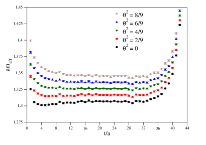
Figure 1: Effective mass plots of the $\eta_{c}$-meson with the fit of Eq. 3 for the ensemble H101.

II.3 Chosen measurements and correlation functions

To make sure that we are using observables that are sensitive to all of the parameters in the RHQ action, we will be using both S- and P-wave charmonium ground-state masses (listed in Tab. 2) in addition to the dispersion relation for the spin-averaged S-wave ground state. A possibility that would make this dependence a bit more obvious would have been to focus on the 1S hyperfine splitting, along with the S-wave – P-wave splitting, the spin-orbit splitting and the tensor splitting within the P-wave, as for example used in [37, 9]. For computational reasons, we instead restrict the interpolator basis to the states that can be reached using the simple mesonic operators at rest,

$$O(x)=(\bar{\psi}\Gamma\psi)(x),$$ (4)

and compare these directly with their continuum analogs. Note that the $J^{PC}=1^{+-}$ $h_{c}$ is however a good proxy for the spin-average of the 1P states, as the 1P hyperfine splitting is expected to be very small [38] (which can also be seen in a previous lattice determination [9]). Throughout, we will use gauge-fixed wall sources with Gaussian sink-smearing implemented by the method discussed in App. B to optimise for the ground states and those with twisting. An example of our zero-momentum states can be found in Fig. 2 for the ensemble N202.

State	$\eta_{c}$	$J/\psi$	$\chi_{c0}$	$\chi_{c1}$	$h_{c}$
$\Gamma$	$\gamma_{5}$	$\gamma_{i}$	$I$	$\gamma_{i}\gamma_{t}$	$\gamma_{i}\gamma_{j}$
$J^{PC}$	$0^{-+}$	$1^{--}$	$0^{++}$	$1^{++}$	$1^{+-}$
Experiment [GeV]	2.9839	3.096916	3.41471	3.51072	3.52549

Table 2: List of operators used in our measurement of charmonium, their expected quantum number equivalents to continuum states and the experimental masses of these states [39].

For the open-boundary ensembles we perform a single wall-source propagator inversion at $T/2$, in the middle of the bulk, and symmetrise the resulting correlator. We must make sure to not perform our fits too close to the open boundary as these boundary-effects can be relatively strong, as seen in Fig. 1.

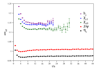
Figure 2: Effective masses of the states listed in Tab. 2 for the ensemble N202.

II.4 Neural-network charm-action tuning

Our idea is to randomly choose values of $\kappa_{c},r_{s},\nu,c_{E},$ and $c_{B}$ and measure the basic spectrum of Tab. 2 on a sufficient number of gauge configurations. We will then train a neural network in predicting these parameters for given input masses and $c^{2}$, and finally use this model to predict the best guesses for the parameters of the action that lie closest to the experimental masses with spin-averaged $c^{2}=1$, hopefully within a precision of $1\%$. We acknowledge that all of the states will likely have residual cut-off effects with different slopes but the parameters of the action should be able to absorb the leading cut-off effects [5, 6]. As we approach the (chiral-)continuum limit the states from the predicted parameters tend to the continuum masses, by design.

We strived to have at least about 30 different sets of run parameters randomly drawn from initially broad Gaussian distributions per ensemble . For some ensembles we performed more runs to investigate the possible inter-ensemble dependencies, such as those emanating from the pion mass or the volume. Typically, after about 20 runs we start refining our parameter space by narrowing the new trial parameters and by feeding guesses back into the system to accelerate convergence. For each state entering the network we use 1000 bootstraps, which will both help give the network lots of data to train against and inform it of correlations between states.

We will first consider each individual ensemble separately to train the network, eventually investigating combinations of ensembles and performing more-global fits. We initially have 6 input parameters: the lattice determinations of the $\eta_{c},J/\psi,\chi_{c0},\chi_{c1},$ and $h_{c}$ mesons, and the lattice $\eta_{c}-J/\psi$ spin-averaged dispersion relation $c^{2}$. We will use a feed-forward network with one hidden layer of only 12 neurons and an output layer of 5 neurons ($\kappa_{c},r_{s},\nu,c_{E},$ and $c_{B}$). On each of the layers we use the sigmoid activation and the Adam minimiser, with an adjusted learning rate, early-stopping, and a batch-size of 80. With the loss-function set as the mean-squared deviation. Often the model will converge rapidly to stable training and validation losses in fewer than 200 epochs.

Once the network understands the relation between the lattice-determined states and the charm-action parameters on an ensemble, we determine the best finite-lattice-spacing approximation to the action parameters needed to obtain something close to the experimental states with $c^{2}=1$ from the spin-averaged dispersion relation. Initial studies indicated that this approach gave predictions with heavier-than-physical $\eta_{c}$ and $\chi_{c0}$ states, and we decided to introduce so-called ”class weights” to tell the network to prefer tuning $\kappa_{c}$ by a factor of 2 compared to the other outputs. Empirically, this makes the $\eta_{c}$ and $\chi_{c0}$ closer to physical while making the $\chi_{c1}$ and $h_{c}$ and $c^{2}$ a little less accurate, as will be seen in Fig. 4.

For the selection of our training and validation sets we randomly shuffle the runs and remove approximately $20\%$ for validation. We run the training over 50 of these reshufflings and perform a weighted average (with weight proportional to the inverse of the validation loss) of the networks’ best guesses to determine our predictions. In the following (Tab. 3) we quote our predicted parameters with $1\sigma$ errors, although this should not be construed as a true error but rather an indication of the variation of the parameters within the training runs we performed.

III Results

III.1 Table of predictions

Ensemble	Runs	$\kappa_{c}$	$c_{E}$	$c_{B}$	$r_{s}$	$\nu$
A653	41	0.10951(09)	2.150(16)	2.313(28)	1.1645(34)	1.1515(40)
A654	33	0.10939(06)	2.110(11)	2.290(13)	1.1709(39)	1.1609(24)
Comb	74	0.10946(04)	2.138(09)	2.305(13)	1.1672(23)	1.1563(25)
U103	40	0.11409(09)	1.982(06)	2.139(15)	1.1375(13)	1.1229(16)
H101	40	0.11436(10)	1.925(11)	2.112(18)	1.1412(22)	1.1222(16)
H102	45	0.11447(07)	1.894(12)	2.032(16)	1.1454(20)	1.1098(28)
H105	40	0.11450(09)	1.937(08)	2.093(09)	1.1376(22)	1.1144(19)
Comb	165	0.11434(06)	1.940(07)	2.102(12)	1.1395(18)	1.1167(23)
B450	34	0.11826(10)	1.890(08)	2.051(08)	1.1017(23)	1.0849(36)
S400	35	0.11796(09)	1.880(10)	2.060(12)	1.1073(17)	1.0924(19)
N451	23	0.11835(10)	1.907(09)	2.025(07)	1.1020(15)	1.0950(20)
Comb	92	0.11810(04)	1.894(04)	2.052(05)	1.1043(12)	1.0926(12)
H200	36	0.12248(11)	1.864(09)	1.894(07)	1.0683(22)	1.0518(29)
N202	36	0.12256(20)	1.865(08)	1.889(10)	1.0679(13)	1.0446(24)
N203	36	0.12232(06)	1.863(09)	1.879(11)	1.0733(09)	1.0605(11)
N200	36	0.12211(09)	1.860(08)	1.888(06)	1.0753(09)	1.0564(15)
Comb	144	0.12235(05)	1.859(05)	1.886(04)	1.0722(09)	1.0552(08)
N300	50	0.12608(15)	1.792(15)	1.873(14)	1.0382(13)	1.0168(19)

Table 3: Charm-action parameter predictions for our data, the quantities in brackets are one-sigma variations in the predicted parameters, see text for details. ”Comb” refers to the prediction from the neural-network when combining all results with a given lattice spacing. Different lattice spacings are separated by double horizontal lines.

In Tab. 3 we present our results for the tuning on individual ensembles as well as a combined data-set built from the individual ones at fixed lattice spacing, which is practically an assumption of a flat approach to physical light and strange quark masses, combined with the (likely justified) assumption that finite volume effects in our charmonium observables are not relevant for our volumes. Typically the loss from the neural network reduces when the larger data-set ”Comb” is used, and this larger data-set should protect us a little more from over-fitting.

Comparing our results to the similar tuning of [28] ($\kappa_{c}=0.10959947$, $c_{E}=1.7819512$, $c_{B}=1.9849139$, $r_{s}=1.1881607$, and $\nu=1.1450511$) albeit on different ensembles, we see some similarities and a few differences. Namely, that at a similar lattice spacing to theirs ($a^{-1}=2.194\text{ GeV}$), our 1-ensembles, the values we obtain for $\kappa_{c},c_{E}$, and $c_{B}$ are larger, while both $r_{s}$ and $\nu$ are smaller. Our larger values of $c_{E}$ and $c_{B}$ are unsurprising as the gauge fields used are generated with the tree-level Symanzik gauge action whereas they used the Iwasaki, and the size of the non-perturbative $c_{\text{SW}}$ is larger for the Symanzik gauge action at comparable lattice spacing. It is interesting to note that their values for $\kappa_{c},r_{s}$, and $\nu$ resemble more our tuning parameters on the coarser ensembles A653 and A654.

It is clear from Tab. 3 that as the lattice-spacing reduces the size of all of the parameters $c_{E},c_{B},r_{s},$ and $\nu$ also decrease. With $r_{s}$ and $\nu$ practically tending to their expected continuum values of 1. Both of the parameters $c_{E}$ and $c_{B}$ are greater than the value of (but tending toward) $c_{\text{SW}}$ from [42], with the hierarchy of $c_{B}>c_{E}$ as expected perturbatively from [22].

III.2 On the validity of fixing parameters and tuning others

As $c^{2}=1$ from the spin-averaged dispersion relation is one of our inputs we can use this as a handle and investigate the dependence on the predicted physical parameters as this value is varied (and all the other states are still set to their physical values). If the deviation on $\kappa_{c},r_{s},c_{E},c_{B},$ and $\nu$ is large as small changes are applied to this dispersion relation, then the model is suggesting that there is significant inter-dependence between these parameters and that this tuning shouldn’t be done independently, as was performed in [28].

Fig. 3 illustrates the normalised deviation for some model-predicted parameter P, which we define as,

$$N[c^{2}]=(P[c^{2}]-P[1])/P[1],$$ (5)

for the combined $A653$ and $A654$ ensembles as we varied the spin-averaged dispersion relation’s $c^{2}$. We can see that $\kappa_{c}$ and $r_{s}$ do not depend strongly on $c^{2}$ whereas $\nu,c_{E},$ and $c_{B}$ do. With $c_{E}$ and $c_{B}$ being somewhat anti-correlated with $\nu$. Although $\nu$ seems to be the main perpetrator in determining the effective speed of light, $c_{E}$ and $c_{B}$ both change accordingly and would likely need to be re-tuned to accommodate an independent tuning in $\nu$.

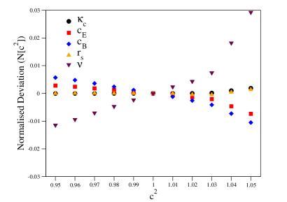
Figure 3: The predicted normalised deviation of the parameters as we change the effective spin-averaged speed of light.

III.3 Accuracy of our predictions and systematics

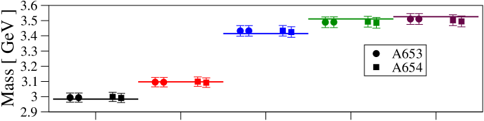
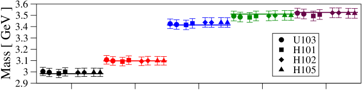
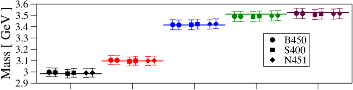
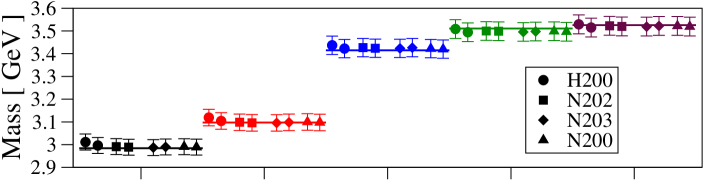
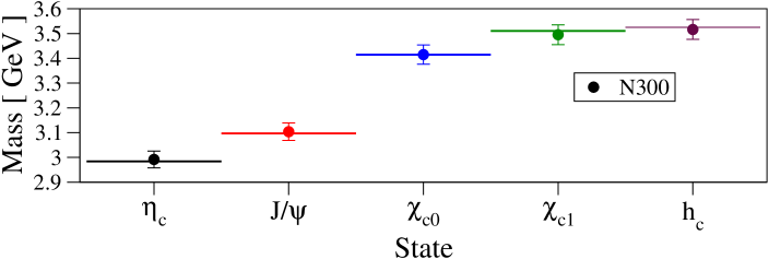
Figure 4: Overview of the resulting masses for the hadrons used for our neural net tuning. The horizontal lines show the experiment masses. The uncertainty combines statistical and scale-setting uncertainties in quadrature, and the uncertainty is dominated by the scale setting. The panes are sorted from coarsest (top) to finest (bottom) lattice spacing. For each ensemble two results are shown: the tuning on the single ensemble (left symbol) and the tuning on the collection of ensembles with the same $\beta$ (right symbol). Ensembles within the same panel differ by volume and/or pion mass.

We now proceed to test our predicted parameters from Tab. 3 by performing the same measurement runs on the same configurations as the training was performed on, and comparing the determined states and the effective speed of light to the physical continuum states. We will investigate both the combined and the individual results to illustrate the lack of measurable dependence on the pion mass within the precision of our determinations. A plot of our ability to reproduce the spectrum is shown in Fig. 4 and one can see that within our large errors there is good agreement, mostly this is due to the lack of precision of our lattice spacing.

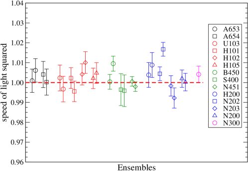
Figure 5: Spin-averaged $c^{2}$ reached through our tuning prescription. For each ensemble a pair of data points is shown. The left data point result from the tuning on the single ensemble, while the right data point results from the tuning using all ensembles with the same lattice spacing.

Fig. 5 shows the spin-averaged $c^{2}$ reached for our tuning procedure on all ensembles. For each ensemble we show both the result from the tuning procedure on a single ensemble (the left point of the pair) and the result from using all ensembles at the same value of $\beta$ (the right point of a given pair). Our overall goal here was to to obtain $c^{2}=1$ to about 1%, which we achieve on most ensembles. For the dispersion relation, the single-ensemble tuning works a bit better than combining ensembles at each lattice spacing. However, the opposite will be true for the splitting discussed in the next few paragraphs. Note, that while there are some outliers, the situation is vastly improved compared to a standard Wilson-action ($c_{B}=c_{E}=c_{sw}$, and $r_{s}=r_{t}=\nu=1$) as used for the charm quark in [17], and discussed in the next sub-section (Sec. III.4).

To investigate residual discretisation effects within our approach, we take a look at the mass-splittings among our tuning states. In the left-hand-side panel of Fig. 6 we show the 1S hyperfine splitting between the $J/\psi$ and $\eta_{c}$ mesons resulting from the neural net training with all ensembles at a given value of $\beta$. While the run parameters suggested by the neural net based on the training data do not lead to a particularly accurate 1S hyperfine splitting at coarse lattice spacing, this discrepancy does get smaller towards the continuum limit. This suggests that our strategy of using the physical inputs for the tuning of the action parameters at each lattice spacing is working. In addition to the data from our final runs we also show the PDG value [39] as a magenta star, and an independent lattice determination that provides this splitting as a prediction [9]. For a plot of further results for this quantity see Fig. 8 of the same reference.

The right hand side of Fig. 6 shows a mass-splitting which is equal to the S-wave – P-wave splitting in the absence of a P-wave hyperfine splitting. In this quantity we expect a very mild heavy-quark dependence, as the physical S-wave – P-wave splittings in charmonium and bottomonium are almost the same. Just like for the hyperfine splitting, there is no obvious sign of issues with our tuning approach. Overall we tend to get somewhat smaller values for this splitting, although with large errors coming from our determination of $h_{c}$. As our application for this action will mostly be qualitative studies of hadron-hadron scattering, we currently see no need to attempt to further improve the observed behaviour, which would require an improvement in statistical precision on our side combined with an improvement in the determination of the lattice spacing.

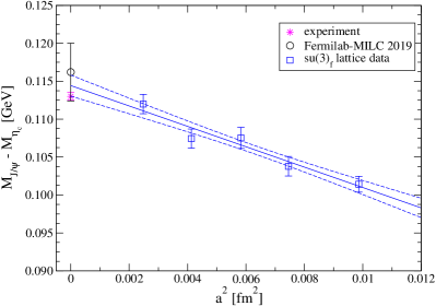
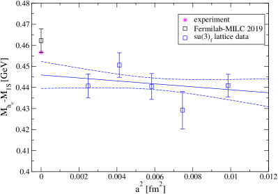
Figure 6: Left panel: 1S hyperfine splitting on the trajectory with $m_{u/d}=m_{s}$ corresponding to the heaviest pion masses (choosing the largest volume) in Tab. 1. The splitting is clearly tending towards the physical splitting for small lattice spacing. The blue lines and blue dashed error band show the results of a fit linear in the lattice spacing squared, which is compatible with the presence of such sub-leading discretisation effects in our action. Right panel: A proxy for the S-wave – P-wave splitting along the same line. Note that both results are not determinations and instead illustrate the quality and suitability of our tuning.

III.4 A tuning comparison on the same ensembles

In [17] a charm-quark tuning was performed that uses $c_{E}=c_{B}=c_{\text{SW}}$ and $r_{s}=\nu=1$, varying $\kappa_{c}$ to achieve the physical continuum value of the $D_{s}$-meson mass on the same ensembles as used in this work. This tuning treats the charm-quark on the same footing as the light and strange quarks by using the standard Wilson-clover action, one may well expect this to have significant discretisation effects as $aM_{\eta_{c}}$ becomes of order 1 for the coarse ensembles.

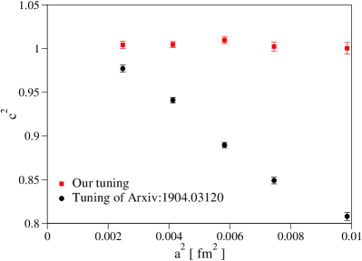
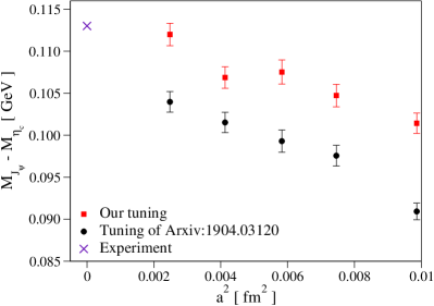
Figure 7: (Left) the speed of light squared from the spin-averaged dispersion relation using either the charm-quark tuning of [17] or our tuning on ensembles at the $\text{SU}(3)_{f}$-symmetric point. (Right) the hyperfine splitting for the two tunings.

Fig. 7 illustrates the deviation of the spin-averaged dispersion relation $c^{2}$, which can be used as a proxy for the magnitude of discretisation effects of both tunings. In the dispersion relation for the $D_{s}$-tuning the deviation from 1 is at most $20\%$ reducing to about $4\%$ on the finest (N300) lattice. A naive, straight-line fit through all of the $D_{s}$-tuned results describes the data poorly and over-predicts the value of $c^{2}$ in the continuum as there is still some visible curvature at small $a^{2}$. A quadratic fit in $a^{2}$ to the three finest ensembles describes the data well and gives $c^{2}=1$ in continuum.

The hyperfine splitting in Fig. 7 shows a similar slope in $a^{2}$ between the two approaches although the $D_{s}$-tuning lies systematically below that of our tuning and the physical hyperfine splitting. This is due to the ensembles used in this comparison lying at the $\text{SU}(3)_{f}$-symmetric point and the $D_{s}$-tuning compensating for the valence strange being lighter than its physical value. This has the side-effect that a precise charm-tuning via the $D_{s}$ is only valid at the physical point, or through extrapolations toward it when the strange-quark mass is unphysical.

IV Conclusions and outlook

We have shown that it is possible to non-perturbatively determine charm-quark action parameters reasonably precisely using machine learning techniques. This method is appealing as it doesn’t rely on lattice perturbation theory or an underlying model to tune parameters. Its main drawback is that a sufficiently-large number of measurement runs need to be made for training purposes, which could make it costly for large ensembles. Although, at the precision we are able to achieve, we see little pion-mass or finite-volume dependence of our tuning parameters. We also note that it appears impossible to exactly reproduce the chosen continuum states of charmonium at finite lattice spacing with this 5-parameter action, even though a good approximation can be achieved.

We see no reason why this approach couldn’t be extended to, for example, b-quark physics using the same relativistic heavy-quark action. While residual discretisation effects are expected to be sizable for bottomonium [6], this approach should be very useful for refining some older predictions for exotic hadrons in the $B$-meson spectrum [12]. The same approach could equally-well be used to tune an effective action, such as NRQCD, provided one has enough continuum states to compare against that allow for a handle on the underlying simulation parameters. The method presented here, quite naturally, extends to even higher-order heavy-quark actions due to the inherent flexibility of neural-network fits.

In future works we will use this action for scattering studies using Lüscher’s finite-volume method for heavy-light meson spectroscopy and charmonium spectroscopy, with the stochastic distillation technique [43, 44]. In this regard a first step consists of testing the dispersion relations of heavy-light $D$ and $D_{s}$ mesons in our approach.

Appendix A On our charm-action implementation

We use a modified version of the library OpenQCD-1.6 [21] for our computation of propagators for the charm-quark Dirace operator of Eq. II.2. This required the rewriting of the Dirac operator in single and double precision in AVX/FMA vector intrinsics as some of the optimisations (and inline assembly) used in the implementation of the vanilla Wilson action could not be utilised. On paper the arithmetic intensity of this charm action is about a factor of 2 more expensive than the usual Wilson action. Although an optimisation was used here to turn the underlying spinors into color-major, spin-minor order (OpenQCD-1.6 is spin-major, color-minor) to improve cache-coherence and perform fewer shuffling and register loading operations. It is likely that this charm-quark action is worse-conditioned than the usual Wilson action as it is found to have a larger clover term than $c_{\text{SW}}$. Nevertheless, our implementation is roughly comparable to a valence strange quark inversion at physical $m_{s}$ [33] in OpenQCD using the DFL_SAP_GCR algorithm [45].

In initial investigations we found some deviations between charmonium correlators at large times due to the stopping condition of the $L_{2}$-norm of the residual depending on the precision we used. To help resolve this we changed the stopping criteria to be the $L_{\infty}$-norm instead, which empirically behaved much better.

Appendix B Coulomb gauge-fixed box-sinks as a sink smearing

If we consider the box-sink propagator introduced in [33],

$$\tilde{S}(x,t)=\sum_{r=0}^{r^{2}<R^{2}}S(x+r,t),$$ (6)

when one goes to compute the contracted meson there are clearly double-sums and in the limit of $R^{2}\rightarrow 3\frac{L}{2}^{2}$ we are performing two sums over the spatial volume, which becomes very expensive. Empirically, we find the cost in contractions scales quadratically with $R^{2}$, and this sum quickly becomes the dominant cost of contractions as $R^{2}$ increases.

A more-efficient implementation would be to notice that the box-sink approach could be considered as a convolution with a particular step-function, $f(x)=\theta(r<R^{2})$, and herein lies the connection to sink-smearing and a clue to efficient calculation of these propagators. An approximation to this step-function could be a Gaussian with some width $\sigma\propto R^{2}$, $f(x)=e^{-\frac{x^{2}}{\sigma}}$, (although in principle any arbitrary function could be used, for S-wave states something with rotational symmetry makes sense) and we apply the convolution using the usual (fast) Fourier transform prescription,

$$S(p,t)=\mathcal{F}(S(x,t))=\sum_{x}e^{ip\cdot x}S(x,t),$$ (7)

where $\mathcal{F}$ is used to denote the Fourier transform, and likewise $\mathcal{F}^{-1}$ its inverse.

$$\overline{S}(x)=\frac{1}{V}\mathcal{F}^{-1}(S(p,t)f^{*}(p)).$$ (8)

We have turned a somewhat expensive approximate convolution into a full convolution with an arbitrary function $f(x)$, the cost of which are $12\times 12$ complex spatial-volume FFTs per time-slice.

It is important to note that this approach only holds because of the Coulomb gauge-fixed wall sources we use, as only in this case can one treat the links as identity matrices and hence completely ignore them and apply a continuous function. Such approaches have been known in the literature in the case of smearing either the source and/or the sink e.g. applying arbitrary potentials in [46].

References

- Lüscher [1986] M. Lüscher, Volume Dependence of the Energy Spectrum in Massive Quantum Field Theories. 2. Scattering States, Commun. Math. Phys. 105, 153 (1986).
- Lüscher [1991] M. Lüscher, Two particle states on a torus and their relation to the scattering matrix, Nucl. Phys. B354, 531 (1991).
- Briceno et al. [2018] R. A. Briceno, J. J. Dudek, and R. D. Young, Scattering processes and resonances from lattice QCD, Rev. Mod. Phys. 90, 025001 (2018), arXiv:1706.06223 [hep-lat] .
- Sheikholeslami and Wohlert [1985] B. Sheikholeslami and R. Wohlert, Improved Continuum Limit Lattice Action for QCD with Wilson Fermions, Nucl. Phys. B 259, 572 (1985).
- El-Khadra et al. [1997] A. X. El-Khadra, A. S. Kronfeld, and P. B. Mackenzie, Massive fermions in lattice gauge theory, Phys. Rev. D 55, 3933 (1997), arXiv:hep-lat/9604004 .
- Oktay and Kronfeld [2008] M. B. Oktay and A. S. Kronfeld, New lattice action for heavy quarks, Phys. Rev. D 78, 014504 (2008), arXiv:0803.0523 [hep-lat] .
- Bernard et al. [2011] C. Bernard et al. (Fermilab Lattice, MILC), Tuning Fermilab Heavy Quarks in 2+1 Flavor Lattice QCD with Application to Hyperfine Splittings, Phys. Rev. D 83, 034503 (2011), arXiv:1003.1937 [hep-lat] .
- Bailey et al. [2014] J. A. Bailey et al. (Fermilab Lattice, MILC), Update of from the form factor at zero recoil with three-flavor lattice QCD, Phys. Rev. D 89, 114504 (2014), arXiv:1403.0635 [hep-lat] .
- DeTar et al. [2019] C. DeTar, A. S. Kronfeld, S.-h. Lee, D. Mohler, and J. N. Simone (Fermilab Lattice, MILC), Splittings of low-lying charmonium masses at the physical point, Phys. Rev. D 99, 034509 (2019), arXiv:1810.09983 [hep-lat] .
- Lang et al. [2014] C. B. Lang, L. Leskovec, D. Mohler, S. Prelovsek, and R. M. Woloshyn, Ds mesons with DK and D*K scattering near threshold, Phys. Rev. D 90, 034510 (2014), arXiv:1403.8103 [hep-lat] .
- Mohler et al. [2013] D. Mohler, C. B. Lang, L. Leskovec, S. Prelovsek, and R. M. Woloshyn, Meson and -Meson-Kaon Scattering from Lattice QCD, Phys. Rev. Lett. 111, 222001 (2013), arXiv:1308.3175 [hep-lat] .
- Lang et al. [2015a] C. B. Lang, D. Mohler, S. Prelovsek, and R. M. Woloshyn, Predicting positive parity Bs mesons from lattice QCD, Phys. Lett. B 750, 17 (2015a), arXiv:1501.01646 [hep-lat] .
- Lang et al. [2015b] C. B. Lang, L. Leskovec, D. Mohler, and S. Prelovsek, Vector and scalar charmonium resonances with lattice QCD, JHEP 09, 089, arXiv:1503.05363 [hep-lat] .
- Piemonte et al. [2019] S. Piemonte, S. Collins, D. Mohler, M. Padmanath, and S. Prelovsek, Charmonium resonances with and from scattering on the lattice, Phys. Rev. D 100, 074505 (2019), arXiv:1905.03506 [hep-lat] .
- Prelovsek et al. [2021] S. Prelovsek, S. Collins, D. Mohler, M. Padmanath, and S. Piemonte, Charmonium-like resonances with JPC = 0++, 2++ in coupled , scattering on the lattice, JHEP 06, 035, arXiv:2011.02542 [hep-lat] .
- Note [1] For a more thorough description of this procedure see Section IV B. of [14].
- Gérardin et al. [2019] A. Gérardin, M. Cè, G. von Hippel, B. Hörz, H. B. Meyer, D. Mohler, K. Ottnad, J. Wilhelm, and H. Wittig, The leading hadronic contribution to from lattice QCD with flavours of O() improved Wilson quarks, Phys. Rev. D 100, 014510 (2019), arXiv:1904.03120 [hep-lat] .
- Chao et al. [2021] E.-H. Chao, R. J. Hudspith, A. Gérardin, J. R. Green, H. B. Meyer, and K. Ottnad, Hadronic light-by-light contribution to from lattice QCD: a complete calculation, Eur. Phys. J. C 81, 651 (2021), arXiv:2104.02632 [hep-lat] .
- Bruno et al. [2015] M. Bruno et al., Simulation of QCD with N 2 1 flavors of non-perturbatively improved Wilson fermions, JHEP 02, 043, arXiv:1411.3982 [hep-lat] .
- Bali et al. [2016] G. S. Bali, E. E. Scholz, J. Simeth, and W. Söldner (RQCD), Lattice simulations with improved Wilson fermions at a fixed strange quark mass, Phys. Rev. D 94, 074501 (2016), arXiv:1606.09039 [hep-lat] .
- Lüscher and Schaefer [2013] M. Lüscher and S. Schaefer, Lattice QCD with open boundary conditions and twisted-mass reweighting, Comput. Phys. Commun. 184, 519 (2013), arXiv:1206.2809 [hep-lat] .
- Aoki et al. [2004] S. Aoki, Y. Kayaba, and Y. Kuramashi, A Perturbative determination of mass dependent O(a) improvement coefficients in a relativistic heavy quark action, Nucl. Phys. B 697, 271 (2004), arXiv:hep-lat/0309161 .
- Moir et al. [2016] G. Moir, M. Peardon, S. M. Ryan, C. E. Thomas, and D. J. Wilson, Coupled-Channel , and Scattering from Lattice QCD, JHEP 10, 011, arXiv:1607.07093 [hep-lat] .
- Cheung et al. [2016] G. K. C. Cheung, C. O’Hara, G. Moir, M. Peardon, S. M. Ryan, C. E. Thomas, and D. Tims (Hadron Spectrum), Excited and exotic charmonium, and meson spectra for two light quark masses from lattice QCD, JHEP 12, 089, arXiv:1610.01073 [hep-lat] .
- Cheung et al. [2017] G. K. C. Cheung, C. E. Thomas, J. J. Dudek, and R. G. Edwards (Hadron Spectrum), Tetraquark operators in lattice QCD and exotic flavour states in the charm sector, JHEP 11, 033, arXiv:1709.01417 [hep-lat] .
- Cheung et al. [2021] G. K. C. Cheung, C. E. Thomas, D. J. Wilson, G. Moir, M. Peardon, and S. M. Ryan (Hadron Spectrum), DK I = 0,I = 0, 1 scattering and the (2317) from lattice QCD, JHEP 02, 100, arXiv:2008.06432 [hep-lat] .
- Gayer et al. [2021] L. Gayer, N. Lang, S. M. Ryan, D. Tims, C. E. Thomas, and D. J. Wilson (Hadron Spectrum), Isospin-1/2 D scattering and the lightest resonance from lattice QCD, JHEP 07, 123, arXiv:2102.04973 [hep-lat] .
- Namekawa et al. [2011] Y. Namekawa et al. (PACS-CS), Charm quark system at the physical point of 2+1 flavor lattice QCD, Phys. Rev. D 84, 074505 (2011), arXiv:1104.4600 [hep-lat] .
- Namekawa et al. [2013] Y. Namekawa et al. (PACS-CS), Charmed baryons at the physical point in 2+1 flavor lattice QCD, Phys. Rev. D 87, 094512 (2013), arXiv:1301.4743 [hep-lat] .
- Note [2] And similarly for [47] except for the tuning in .
- Aoki et al. [2006] S. Aoki et al. (CP-PACS, JLQCD), Nonperturbative O(a) improvement of the Wilson quark action with the RG-improved gauge action using the Schrödinger functional method, Phys. Rev. D 73, 034501 (2006), arXiv:hep-lat/0508031 .
- Lin and Christ [2007] H.-W. Lin and N. Christ, Non-perturbatively Determined Relativistic Heavy Quark Action, Phys. Rev. D 76, 074506 (2007), arXiv:hep-lat/0608005 .
- Hudspith et al. [2020] R. J. Hudspith, B. Colquhoun, A. Francis, R. Lewis, and K. Maltman, A lattice investigation of exotic tetraquark channels, Phys. Rev. D 102, 114506 (2020), arXiv:2006.14294 [hep-lat] .
- Note [3] Fixed to an accuracy of using the CFACG algorithm [48] implemented in GLU.
- Bedaque [2004] P. F. Bedaque, Aharonov-Bohm effect and nucleon nucleon phase shifts on the lattice, Phys. Lett. B 593, 82 (2004), arXiv:nucl-th/0402051 .
- Sachrajda and Villadoro [2005] C. T. Sachrajda and G. Villadoro, Twisted boundary conditions in lattice simulations, Phys. Lett. B 609, 73 (2005), arXiv:hep-lat/0411033 .
- Burch et al. [2010] T. Burch, C. DeTar, M. Di Pierro, A. X. El-Khadra, E. D. Freeland, S. Gottlieb, A. S. Kronfeld, L. Levkova, P. B. Mackenzie, and J. N. Simone, Quarkonium mass splittings in three-flavor lattice QCD, Phys. Rev. D 81, 034508 (2010), arXiv:0912.2701 [hep-lat] .
- Lebed and Swanson [2017] R. F. Lebed and E. S. Swanson, Quarkonium States As Arbiters of Exoticity, Phys. Rev. D 96, 056015 (2017), arXiv:1705.03140 [hep-ph] .
- Zyla et al. [2020] P. Zyla et al. (Particle Data Group), Review of Particle Physics, PTEP 2020, 083C01 (2020).
- Note [4] To start with, we draw values of and around with a bias towards larger values and a large width, as motivated by perturbation theory. and are initially guessed from a linear fit in from previously-measured ensembles.
- Note [5] We tried many different numbers of layers and neurons in each layer. Enlarging these numbers either did not change predictions compared to the small, simple network, or resulted in what we determined to be over-fitting.
- Bulava and Schaefer [2013] J. Bulava and S. Schaefer, Improvement of = 3 lattice QCD with Wilson fermions and tree-level improved gauge action, Nucl. Phys. B 874, 188 (2013), arXiv:1304.7093 [hep-lat] .
- Peardon et al. [2009] M. Peardon, J. Bulava, J. Foley, C. Morningstar, J. Dudek, R. G. Edwards, B. Joo, H.-W. Lin, D. G. Richards, and K. J. Juge (Hadron Spectrum), A Novel quark-field creation operator construction for hadronic physics in lattice QCD, Phys. Rev. D 80, 054506 (2009), arXiv:0905.2160 [hep-lat] .
- Morningstar et al. [2011] C. Morningstar, J. Bulava, J. Foley, K. J. Juge, D. Lenkner, M. Peardon, and C. H. Wong, Improved stochastic estimation of quark propagation with Laplacian Heaviside smearing in lattice QCD, Phys. Rev. D 83, 114505 (2011), arXiv:1104.3870 [hep-lat] .
- Lüscher [2007] M. Lüscher, Local coherence and deflation of the low quark modes in lattice QCD, JHEP 07, 081, arXiv:0706.2298 [hep-lat] .
- Davies et al. [1994] C. T. H. Davies, K. Hornbostel, A. Langnau, G. P. Lepage, A. Lidsey, J. Shigemitsu, and J. H. Sloan, Precision Upsilon spectroscopy from nonrelativistic lattice QCD, Phys. Rev. D 50, 6963 (1994), arXiv:hep-lat/9406017 .
- Kayaba et al. [2007] Y. Kayaba, S. Aoki, M. Fukugita, Y. Iwasaki, K. Kanaya, Y. Kuramashi, M. Okawa, A. Ukawa, and T. Yoshié (CP-PACS), First Nonperturbative Test of a Relativistic Heavy Quark Action in Quenched Lattice QCD, JHEP 02, 019, arXiv:hep-lat/0611033 .
- Hudspith [2015] R. J. Hudspith (RBC, UKQCD), Fourier Accelerated Conjugate Gradient Lattice Gauge Fixing, Comput. Phys. Commun. 187, 115 (2015), arXiv:1405.5812 [hep-lat] .