CoNeRF: Controllable Neural Radiance Fields

Abstract

We extend neural 3D representations to allow for intuitive and interpretable user control beyond novel view rendering (i.e. camera control). We allow the user to annotate which part of the scene one wishes to control with just a small number of mask annotations in the training images. Our key idea is to treat the attributes as latent variables that are regressed by the neural network given the scene encoding. This leads to a few-shot learning framework, where attributes are discovered automatically by the framework, when annotations are not provided. We apply our method to various scenes with different types of controllable attributes (e.g. expression control on human faces, or state control in movement of inanimate objects). Overall, we demonstrate, to the best of our knowledge, for the first time novel view and novel attribute re-rendering of scenes from a single video.

1 Introduction

Neural radiance field (NeRF) [30] methods have recently gained popularity thanks to their ability to render photorealistic novel-view images [28, 35, 36, 49]. In order to widen the scope to other possible applications, such as digital media production, a natural question is whether these methods could be extended to enable direct and intuitive control by a digital artist, or even a casual user. However, current techniques only allow coarse-grain controls over materials [52], color [18], or object placement [47], or only support changes that they are designed to deal with, such as shape deformations on a learned shape space of chairs [25], or are limited to facial expressions encoded by an explicit face model [12]. By contrast, we are interested in fine-grained control without limiting ourselves to a specific class of objects or their properties. For example, given a self-portrait video, we would like to be able to control individual attributes (e.g. whether the mouth is open or closed); see Figure LABEL:fig:teaser. We would like to achieve this objective with minimal user intervention, without the need of specialized capture setups [24].

However, it is unclear how fine-grained control can be achieved, as current state-of-the-art models [36] encode the structure of the 3D scene in a single and not interpretable latent code. For the example of face manipulation, one could attempt to resolve this problem by providing dense supervision by matching images to the corresponding Facial Action Coding System (FACS) [11] action units. Unfortunately, this would require either an automatic annotation process or careful and extensive per-frame human annotations, making the process expensive, generally unwieldy, and, most importantly, domain-specific. Automated tools for domain-agnostic latent disentanglement are a very active topic of research in machine learning [17, 16, 9], but no effective plug-and-play solution exists yet.

Conversely, we borrow ideas from 3D morphable models (3DMM) [7], and in particular to recent extensions that achieve local control by spatial disentanglement of control attributes [45, 32]. Rather than having a single global code controlling the expression of the entire face, we would like to have a set of local “attributes”, each controlling the corresponding localized appearance; more specifically, we assume spatial quasi-conditional independence of attributes [45]. For our example in Figure LABEL:fig:teaser, we seek an attribute capable to control the appearance of the mouth, another to control the appearance of the eye, etc.

Thus, we introduce a learning framework denoted CoNeRF (i.e. Controllable NeRF) that is capable of achieving this objective with just few-shot supervision. As illustrated in Figure LABEL:fig:teaser, given a single one-minute video, and with as little as two annotations per attribute, CoNeRF allows fine-grained, direct, and interpretable control over attributes. Our core idea is to provide, on top of the ground truth attribute tuple, sparse 2D mask annotations that specify which region of the image an attribute controls. Further, by treating attributes as latent variables within the framework, the mask annotations can be automatically propagated to the whole input video. Thanks to the quasi-conditional independence of attributes, our technique allows us to synthesize expressions that were never seen at training time; e.g. the input video never contained a frame where both eye were closed and the actor had a smiling expression; see Figure LABEL:fig:teaser (green box).

Contributions

To summarize, our CoNeRF method:

• provides direct, intuitive, and fine-grained control over 3D neural representations encoded as NeRF;

• achieves this via few-shot supervision, e.g., just a handful of annotations in the form of attribute values and corresponding 2D mask are needed for a one minute video;

• while inspired by domain-specific facial animation research [45], it provides a domain-agnostic technique.

2 Related works

Neural Radiance Fields [30] provide high-quality renderings of scenes from novel views with just a few exemplar images captured by a handheld device. Various extensions have been suggested to date. These include ones that focus on improving the quality of results [28, 35, 36, 49], ones that allow a single model to be used for multiple scenes [39, 43], and some considering controllability of the rendering output at a coarse level [14, 48, 25, 47, 46, 52], as we detail next.

In more detail, existing works enable only compositional control of object location [47, 48], and recent extensions also allow for finer-grain reproduction of global illumination effects [14]. NeRFactor [52] shows one can model albedos and BRDFs, and shadows, which can be used to, e.g., edit material, but the manipulation they support is limited to what is modeled through the rendering equation. CodeNeRF [18] and EditNeRF [25] showed that one can edit NeRF models by modifying the shape and appearance encoding, but they require a curated dataset of objects viewed under different views and colors. HyperNeRF [36], on the other hand can adapt to unseen changes specific to the scene, but learns an arbitrary attribute (ambient) space that cannot be supervised, and, as we show in Section 4, cannot be easily related to specific local attribute within the scene for controllability.

Explicit supervision

One can also condition NeRF representations [12] with face attribute predicted by pre-trained face tracking networks, such as Face2Face [41]. Similarly, for human bodies, A-NeRF [40] and NARF [33] use the SMPL [26] model to generate interpretable pose parameters, and Neural Actor [24] further includes normal and texture maps more detailed rendering. While these models result in controllable NeRF, they are limited to domain-specific control and the availability of a heavily engineered control model.

Controllable neural implicits

Controllability of neural 3D implicit representations has also been addressed by the research community. Many works have limited focus on learning human neural implicit representations while enabling the control via SMPL parameters [26], or linear blend skinning weights [53, 15, 38, 29, 27, 10, 4, 54]. Some initial attempts at learned disentangled of shape and poses have also been made in A-SDF [31], allowing behavior control of the output geometry (e.g. doors open vs. closed) while maintaining the general shape. However, the approach is limited to controlling $\text{SE}(3)$ articulation of objects, and requires dense 3D supervision.

2.1 Neural Radiance Field (NeRF)

For completeness, we briefly discuss NeRF before diving into the details of our method. A Neural Radiance Field captures a volumetric representation of a specific scene within the weights of a neural network. As input, it receives a sample position ${\mathbf{x}}$ and a view direction ${\mathbf{v}}$ and outputs the density of the scene $\sigma$ at position ${\mathbf{x}}$ as well as the color ${\mathbf{c}}$ at position ${\mathbf{x}}$ as seen from view direction ${\mathbf{v}}$. One then renders image pixels ${\mathbf{C}}$ via volume rendering [19]. In more detail, ${\mathbf{x}}$ is defined by observing rays ${\mathbf{r}}(t)$ as ${\mathbf{x}}={\mathbf{r}}(t)$, where $t$ parameterizes at which point of the ray you are computing for. One then renders the color of each pixel ${\mathbf{C}}({\mathbf{r}})$ by computing

$${\mathbf{C}}\left({\mathbf{r}}\right)=\int_{t_{n}}^{t_{f}}T(t)\sigma\left({\mathbf{r}}(t)\right){\mathbf{c}}\left({\mathbf{r}}(t),{\mathbf{v}}\right)dt\;,$$ (1)

where ${\mathbf{v}}$ is the viewing angle of the ray ${\mathbf{r}}$, $t_{n}$ and $t_{f}$ are the near and far planes of the rendering volume, and

$$T(t)=\exp\left(-\int_{t_{n}}^{t}\sigma({\bf r}(s))ds\right)\;,$$ (2)

is the accumulated transmittance. Integration in (1) is typically done via numerical integration [30].

2.2 HyperNeRF

Note that in its original formulation (1) is only able to model static scenes. Various recent works [35, 36, 42] have been proposed to explicitly account for possible appearance changes in a scene (for example, temporal changes in a video). To achieve this, they introduce the notion of canonical hyperspace – more formally given a 3D query point ${\mathbf{x}}$ and the collection $\boldsymbol{\theta}$ of all parameters that describe the model, they define:

$${\mathcal{K}}({\mathbf{x}}) \equiv{\mathcal{K}}({\mathbf{x}}\leavevmode\nobreak\ |\leavevmode\nobreak\ {\boldsymbol{\beta}},\boldsymbol{\theta}),\quad$$ Canonicalizer (3)

$${\boldsymbol{\beta}}({\mathbf{x}}) \equiv\mathcal{H}({\mathbf{x}}\leavevmode\nobreak\ |\leavevmode\nobreak\ {\boldsymbol{\beta}},\boldsymbol{\theta}),\quad$$ Hyper Map (4)

$${\mathbf{c}}(\mathbf{x}),\sigma(\mathbf{x}) ={\mathcal{R}}({\mathcal{K}}({\mathbf{x}}),{\boldsymbol{\beta}}({\mathbf{x}})\leavevmode\nobreak\ |\leavevmode\nobreak\ \boldsymbol{\theta}).\quad$$ Hyper NeRF (5)

where the location is canonicalized via a canonicalizer ${\mathcal{K}}$, and the appearances, represented by ${\boldsymbol{\beta}}$, are mapped to a hyperspace via $\mathcal{H}$, which are then utilized by another neural network ${\mathcal{R}}$ to retrieve the color ${\mathbf{c}}$ and the density $\sigma$ at the query location. Note throughout this paper we denote $\boldsymbol{\beta}$ to indicates a latent code, while $\boldsymbol{\beta}(\mathbf{x})$ to indicate the corresponding field generated by the hypermap lifting. With this latent lifting, these methods render the scene via Eq. (1). Note that the original NeRF model can be thought of the case where ${\mathcal{K}}$ and $\mathcal{H}$ are identity mappings.

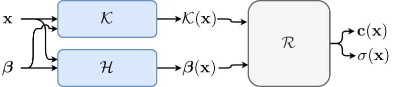
(a) Neural radiance field with lifting [36]

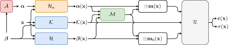
(b) Controllable neural radiance field (our method)

Figure 1: Framework – We depict in (a) the HyperNeRF [36] formulation, and (b) our Controllable-NeRF (CoNeRF). In (a), both point coordinates $\mathbf{x}$ and latent representation $\boldsymbol{\beta}$ are respectively processed by a canonicalizer ${\mathcal{K}}$ and a hyper map $\mathcal{H}$, which are then turned into radiance and density field values by ${\mathcal{R}}$. In (b), we introduce regressors ${\mathcal{A}}$ and $\mathcal{M}$ that regress the attribute and the corresponding mask that enable few-shot attribute-based control of the NeRF model. See Section 3.3 for details.

3 Controllable NeRF (CoNeRF)

Given a collection of $C$ color images $\{\mathbf{C}_{c}\}\in[0,1]^{0pt\times 0pt\times 3}$, we train our controllable neural radiance field model by an auto-decoding optimization [34] whose losses can be grouped into two main subsets:

$$\operatorname*{arg\,min}_{\boldsymbol{\theta}=\boldsymbol{\theta},\{\boldsymbol{\beta}_{c}\}}\underbrace{\mathcal{L}_{\text{rep}}(\boldsymbol{\theta}\leavevmode\nobreak\ |\leavevmode\nobreak\ \{\mathbf{C}_{c}\})}_{\text{Section\leavevmode\nobreak\ \ref{sec:autodecode}}}{+}\underbrace{\mathcal{L}_{\text{ctrl}}(\boldsymbol{\theta}\leavevmode\nobreak\ |\leavevmode\nobreak\ \{\mathbf{M}^{\text{gt}}_{c,a}\},\{\alpha^{\text{gt}}_{c,a}\})}_{\text{Section\leavevmode\nobreak\ \ref{sec:control}}}.$$ (6)

The first group consists of the classical HyperNeRF [36] auto-decoder losses, attempting to optimize neural network parameters $\boldsymbol{\theta}$ jointly with latent codes $\{\boldsymbol{\beta}_{c}\}$ to reproduce the corresponding input images $\{\mathbf{C}_{c}\}$:

$$\mathcal{L}_{\text{rep}}(\cdot)=\mathcal{L}_{\text{recon}}(\boldsymbol{\theta},\{\boldsymbol{\beta}_{c}\}\leavevmode\nobreak\ |\leavevmode\nobreak\ \{\mathbf{C}_{c}\})+\mathcal{L}_{\text{enc}}(\{\boldsymbol{\beta}_{c}\}).$$ (7)

The latter allow us to inject explicit control into the representation, and are our core contribution:

$$\mathcal{L}_{\text{ctrl}}(\cdot) =\mathcal{L}_{\text{mask}}(\boldsymbol{\theta},\{\boldsymbol{\beta}_{c}\}\leavevmode\nobreak\ |\leavevmode\nobreak\ \{\mathbf{M}^{\text{gt}}_{c,a}\})$$ g.t. masks (8)

$$+\mathcal{L}_{\text{attr}}(\boldsymbol{\theta},\{\boldsymbol{\beta}_{c}\}\leavevmode\nobreak\ |\leavevmode\nobreak\ \{\alpha^{\text{gt}}_{c,a}\}).$$ g.t. attributes (9)

As mentioned earlier in Section 1, we aim for a neural 3D appearance model that is controlled by a collection of attributes $\boldsymbol{\alpha}{=}\{\alpha_{a}\}$, and we expect each image to be a manifestation of a different value of attributes, that is, each image $\mathbf{C}_{c}$, and hence each latent code $\boldsymbol{\beta}_{c}$, will have a corresponding attribute $\boldsymbol{\alpha}_{c}$. The learnable connection between latent codes $\boldsymbol{\beta}$ and the attributes $\boldsymbol{\alpha}$, which we represent via regressors, is detailed in Section 3.3.

3.1 Reconstruction losses

The primary loss guiding the training of the NeRF model is the reconstruction loss, which simply aims to reconstruct observations $\{\mathbf{C}_{c}\}$. As in other neural radiance field models [30, 28, 35, 36] we simply minimize the L2 photometric reconstruction error with respect to ground truth images:

$$\mathcal{L}_{\text{recon}}(\cdot)=\sum_{c}\mathbb{E}_{{\mathbf{r}}\sim\mathbf{C}_{c}}\left[\left\|{\mathbf{C}}({\mathbf{r}}\leavevmode\nobreak\ |\leavevmode\nobreak\ \boldsymbol{\beta}_{c},\boldsymbol{\theta})-{\mathbf{C}}^{\text{gt}}({\mathbf{r}})\right\|_{2}^{2}\right].$$ (10)

As is typical in auto-decoders, and following [34], we impose a zero-mean Gaussian prior on the latent codes $\{\boldsymbol{\beta}_{c}\}$:

$$\mathcal{L}_{\text{enc}}(\cdot)=\sum_{c}\left\|\boldsymbol{\beta}_{c}\right\|^{2}_{2}.$$ (11)

3.2 Control losses

The user defines a discrete set of $A$ number of attributes that they seek to control, that are sparsely supervised across frames—we only supervise attributes when we have an annotation, and let others be discovered on their own throughout the training process, as guided by (7). More specifically, for a particular image $\mathbf{C}_{c}$, and a particular attribute $\alpha_{a}$, the user specifies the quantities:

• $\alpha_{c,a}\in[-1,1]$: specifying the value for the $a$-th attribute in the $c$-th image; see the sliders in Figure LABEL:fig:teaser;

• $\mathbf{M}_{c,a}\in[0,1]^{0pt\times 0pt}$: roughly specifying the image region that is controlled by the $a$-th attribute in the $c$-th image; see the masks in Figure LABEL:fig:teaser.

To formalize sparse supervision, we employ an indicator function $\delta_{c,a}$, where $\delta_{c,a}=1$ if an annotation for attribute $a$ for image $c$ is provided, otherwise $\delta_{c,a}=0$. We then write the loss for attribute supervision as:

$$\mathcal{L}_{\text{attr}}(\cdot)=\sum_{c}\sum_{a}\delta_{c,a}|\alpha_{c,a}-\alpha^{\text{gt}}_{c,a}|^{2}.$$ (12)

For the mask few-shot supervision,  we employ the volume rendering in (20) to project the 3D volumetric neural mask field $\mathbf{m}_{a}({\mathbf{x}})$ into image space, and then supervise it as:

$$\mathcal{L}_{\text{mask}}(\cdot)=\!\!\sum_{c,a}\delta_{c,a}\>\mathbb{E}_{\mathbf{r}}\left[\text{CE}\left(\mathbf{M}({\mathbf{r}}\leavevmode\nobreak\ |\leavevmode\nobreak\ \boldsymbol{\beta}_{c},\boldsymbol{\theta}),\mathbf{M}^{\text{gt}}_{c,a}({\mathbf{r}})\right)\right],$$ (13)

where $\text{CE}\left(\cdot,\cdot\right)$ denotes cross entropy, and the field $\sigma({\mathbf{x}})$ in (20) is learned by minimizing (10). Importantly, as we do not wish for (13) to interfere with the training of the underlying 3D representation learned through (10), we stop gradients in (13) w.r.t. $\sigma({\mathbf{x}})$. Furthermore, in practice, because the attribute mask vs. background distribution can be highly imbalanced depending on which attribute the user is trying to control (e.g. an eye only covers a very small portion of an image), we employ a focal loss [23] in place of the standard cross entropy loss.

3.3 Controlling and rendering images

In what follows, we drop the image subscript $c$ to simplify notation without any loss of generality. Given a latent code $\boldsymbol{\beta}$ representing the 3D scene behind an image, we derive a mapping to our attributes via a neural map ${\mathcal{A}}$ with learnable parameters $\boldsymbol{\theta}$:

$$\{\alpha_{a}\}=\mathcal{A}(\boldsymbol{\beta}\leavevmode\nobreak\ |\leavevmode\nobreak\ \boldsymbol{\theta}),\quad\mathcal{A}:\mathbb{R}^{B}\rightarrow[0,1]^{A},$$ (14)

where these correspond to the sliders in Figure LABEL:fig:teaser. In the same spirit of (4), to allow for complex topological changes that may not be represented by the change in a single scalar value alone, we lift the attributes to a hyperspace. In addition, since each attribute governs different aspects of the scene, we employ per-attribute learnable hypermaps $\{\mathcal{H}_{a}\}$, which we write:

$$\alpha_{a}(\mathbf{x}) =\mathcal{H}_{a}(\mathbf{x},\alpha_{a}\leavevmode\nobreak\ |\leavevmode\nobreak\ \boldsymbol{\theta})\quad\mathcal{H}_{a}:\mathbb{R}^{3}\times\mathbb{R}\rightarrow\mathbb{R}^{d}.$$ (15)

Note that while $\alpha_{a}$ is a scalar value, $\alpha_{a}(\mathbf{x})$ is a field that can be queried at any point $\mathbf{x}$ in space. These fields are concatenated to form $\boldsymbol{\alpha}(\mathbf{x})=\{\alpha_{a}(\mathbf{x})\}$.

We then provide all this information to generate an attribute masking field via a network $\mathcal{M}(\cdot\leavevmode\nobreak\ |\leavevmode\nobreak\ \boldsymbol{\theta})$. This field determines which attribute attends to which position in space $\mathbf{x}$:

$$\mathbf{m}_{0}(\mathbf{x}) \oplus\mathbf{m}(\mathbf{x})=\mathcal{M}({\mathcal{K}}(\mathbf{x}),{\boldsymbol{\beta}}(\mathbf{x}),\boldsymbol{\alpha}(\mathbf{x})\leavevmode\nobreak\ |\leavevmode\nobreak\ \boldsymbol{\theta}),$$ (16)

$$\mathcal{M} :\mathbb{R}^{3}\times\mathbb{R}^{B}\times\mathbb{R}^{A\times d}\rightarrow\mathbb{R}^{A+1}_{+},$$ (17)

where $\oplus$ is a concatenation operator, $\mathbf{m}(\mathbf{x}){=}\{\mathbf{m}_{a}(\mathbf{x})\}$, and the additional mask $\mathbf{m}_{0}(\mathbf{x})$ denotes space that is not affected by any attribute. Note that because the mask location should be affected by both the particular attribute of interest (e.g., the selected eye status) and the global appearance of the scene (e.g., head movement), $\mathcal{M}$ takes both ${\boldsymbol{\beta}}(\mathbf{x})$ and $\boldsymbol{\alpha}(\mathbf{x})$ as input in addition to ${\mathcal{K}}(\mathbf{x})$. In addition, because the mask is modeling the attention related to attributes, collectively, these masks satisfy the partition of unity property:

$$\mathbf{m}_{0}(\mathbf{x})+\Sigma_{a}[\mathbf{m}_{a}(\mathbf{x})]=1\quad\forall\mathbf{x}\in\mathbb{R}^{3}.$$ (18)

Finally, in a similar spirit to (5), all of this information is processed by a neural network that produces the desired radiance and density fields used in volume rendering:

$$\left.\begin{aligned} {\mathbf{c}}(\mathbf{x})\\ \sigma(\mathbf{x})\end{aligned}\right\}\!\!=\!{\mathcal{R}}({\mathcal{K}}(\mathbf{x}),\underbrace{\mathbf{m}(\mathbf{x})\odot\boldsymbol{\alpha}(\mathbf{x})}_{\text{attribute controls}},\underbrace{\mathbf{m}_{0}(\mathbf{x})\cdot\boldsymbol{\beta}(\mathbf{x})}_{\text{everything else}}\leavevmode\nobreak\ |\leavevmode\nobreak\ \boldsymbol{\theta}).$$ (19)

In particular, note that $\mathbf{m}(\mathbf{x}){=}0$ implies $\mathbf{m}_{0}(\mathbf{x}){=}1$, hence our solution has the capability of reverting to classical HyperNeRF (5), where all change in the scene is globally encoded in ${\boldsymbol{\beta}}(\mathbf{x})$. Finally, these fields can be used to render the mask in image space, following a process analogous to volume rendering of radiance:

$$\mathbf{M}({\mathbf{r}}\!\leavevmode\nobreak\ |\leavevmode\nobreak\ \!\boldsymbol{\theta})\!=\!\!\int_{t_{n}}^{t_{f}}\!\!\!\!T(t)\cdot\sigma({\mathbf{r}}(t))\cdot[\mathbf{m}_{0}({\mathbf{r}}(t))\oplus\mathbf{m}({\mathbf{r}}(t))]\,dt.$$ (20)

We depict our inference flow in Figure 1 (b).

3.4 Implementation details

We implement our method for NeRF based on the JAX [8] implementation of HyperNeRF [36]. We use both the scheduled windowed positional encoding and weight initialization of [35], as well as the coarse-to-fine training strategy [36].

Besides the newly added networks, we follow the same architecture as HyperNeRF. For the attribute network ${\mathcal{A}}$ we use a six-layer multi-layer perceptron (MLP) with 32 neurons at each layer, with a skip connection at the fifth layer, following [35, 36]. For the lifting network $\mathcal{H}_{a}$, we use the same architecture as $\mathcal{H}$, except for the input and output dimension sizes. For the masking network $\mathcal{M}$ we use a four-layer MLP with 128 neurons at each layer, followed by an additional 64 neuron layer with a skip connection. The network ${\mathcal{R}}$ also shares the same architecture as HyperNeRF, but with a different input dimension size to accommodate for the changes our method introduces.

2D implementation

To show that our idea is not limited to neural radiance fields, we also test a 2D version of our framework that can be used to directly represent images, without going through volume rendering. We use the same architecture and training procedure as in the NeRF case, with the exception that we do not predict the density $\sigma$, and we also do not have the notion of depth—each ray is directly the pixel. We center crop each video and resize each frame to be $128\times 128$.

Hyperparameters

We train all our NeRF models with $480\times 270$ images and with 128 samples per ray. We train for 250k iterations with a batch size of 512 rays. During training, we also maintain that 10% of rays are sampled from annotated images. We set $\mathcal{L}_{\text{attr}}=10^{-1}$, $\mathcal{L}_{\text{mask}}=10^{-2}$ and $\mathcal{L}_{\text{enc}}=10^{-4}$. For the number of hyper dimensions we set $d=8$. For the experiments with the 2D implementation, we sample 64 random images from the scene and further subsample 1024 pixels from each of them. For all experiments we use Adam [20] with learning rate $10^{-4}$ exponentially decaying to $10^{-5}$, as it reaches 250k iterations. We provide additional architectural details in the supplementary material. Training a single model takes around 12 hours on an NVIDIA V100 GPU.

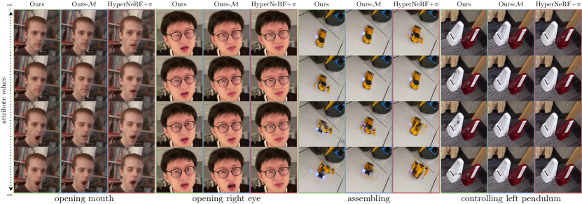
Figure 2: Novel view and novel attribute synthesis on real data – We synthesize scenes from a novel view and with a novel attribute combination, not seen during training. A naive extension of HyperNeRF, HyperNeRF+$\pi$ fails to disentangle attributes and results in a modification of the scene irrespectively of attribute meaning e.g., opening mouth results in closing eyes at the same time. Ours-$\mathcal{M}$ improves the results, but does not disentangles the attribute space, as successfully done by our complete method. The differences between these methods can even lead to complete failure cases, as shown in the metronome and the toy car case.

4 Results

4.1 Datasets and baselines

We evaluate our method on two datasets: real video sequences captured with a smartphone (real dataset) and synthetically rendered sequences (synthetic dataset). Here we introduce those datasets and the baselines for our approach.

Real dataset

Each of the seven real sequences is 1 minute long and was captured either with a Google Pixel 3a or an Apple iPhone 13 Pro. Four of them consists of people performing different facial expressions including smiling, frowning, closing or opening eyes, and opening mouth. For the other three, we captured a toy car changing its shape (a.k.a. Transformer), a single metronome, and two metronomes beating with different rates. For one of the four videos depicting people, to use it for the 2D implementation case, we captured it with a static camera that shows a frontal view of the person. All other sequences feature camera motions showing front and sides of the object in the center of the scene. For videos with human subjects, the subjects signed a participant consent form, which was approved by a research ethics board. We informed the participants that their data will be altered with our method.

We extract frames at 15 FPS which gives approximately 900 frames per capture. Because novel attribute synthesis via user control on real scenes does not have a ground truth view—we aim to create scenes with unseen attribute combinations—the benefit of our method is best seen qualitatively. Nonetheless, to quantitatively evaluate the rendering quality, we interpolate between two frames and evaluate its quality. In more detail, to minimize the chance of the dynamic nature of the scene interfering with this assessment, we use every other frame as a test frame for the interpolation task.

For all human videos, we define three attributes—one for the status of each of the two eyes, and one for the mouth. We annotate only six frames per video in this case, specifically the frames that contain the extremes of each attribute (e.g., left eye fully open). For the toy car, we set the shape of the toy car to be an attribute, and annotate two extremes from two different view points—when the toy is in robot-mode and when it is in car-mode from its left and right side. For the metronomes, we consider the state of the pendulum to be the attribute and annotate the two frames with the two extremes for the single metronome case, and seven frames for the two metronome case as the pendulums of the two metronomes are often close to each other and required special annotations for these close-up cases; see Figure 2.

Synthetic dataset

Since the lack of ground-truth data renders measuring the quality of novel attribute synthesis infeasible in practice, we leverage Kubric software [13] to generate synthetic dataset, where we know exactly the state of each object in the scene. We create a simple scene where three 3D objects, the teapot [3], the Stanford bunny [1], and Suzanne [2], are placed within the scene and are rendered with varying surface colors, which are our attributes; see Figure 4. We generate 900 frames for training and 900 frames for testing. To ensure that the attribute combination during training is not seen in the test scene, we set the attributes to be synchronized for the training split, and desynchronized for the test split. We further render the test split from different camera positions than the training split to account for novel views. We randomly sample 5% of the frames with a given attribute for each object to be set as the ground-truth attribute. During validation, we use attribute values directly to predict the image.

Baselines

To evaluate the reconstruction quality of our method, CoNeRF, we compare it with four different baselines: \raisebox{-.6pt}{1}⃝ standard NeRF [30]; \raisebox{-.6pt}{2}⃝ NeRF+Latent, a simple extension to NeRF where we concatenate each coordinate ${\mathbf{x}}$ with a learnable latent code ${\boldsymbol{\beta}}$ to support appearance changes of the scene; \raisebox{-.6pt}{3}⃝ Nerfies [35]; and \raisebox{-.6pt}{4}⃝ HyperNeRF [36]. Additionally, as existing methods do not support attribute-based control with a few-shot supervision, we create another baseline \raisebox{-.6pt}{5}⃝ by extending HyperNeRF with a simple linear regressor $\pi$ that regresses ${\boldsymbol{\beta}}_{c}$ given ${\boldsymbol{\alpha}}_{c}$. We call this baseline HyperNeRF+$\pi$. To further show the importance of masking, we also compare our approach against a stripped-down version of our method, Ours-$\mathcal{M}$, where we disable the part of our pipeline responsible for masking. All baselines that utilize annotations were trained with the same sparse labels as our method.

4.2 Comparison with the baselines

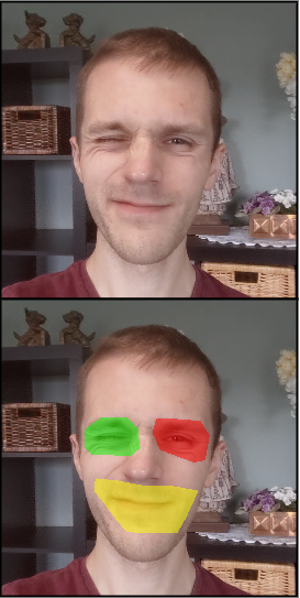
(a) annotation

(b) unannotated views

Figure 3: Annotation example – We provide only a rough annotation for each attribute, which is enough for the method to discover the mask for each attribute across all views automatically. Bottom row shows masks overlaid on the image.

Qualitative highlights

We first show qualitative examples of novel attribute and view synthesis on the real dataset in Figure 2. Our method allows for controlling the selected attribute without changing other aspects of the image—our control is disentangled. This disentanglement allows our method to generate images with attribute combinations that were not seen at training time. On the contrary, as there is no incentive for the learned embeddings of HyperNeRF to be disentangled, the simple regression strategy of HyperNeRF+$\pi$ results in entangled control, where when one tries to close/open the mouth it ends up affecting the eyes. The same phenomenon happens also for Ours-$\mathcal{M}$. Moreover, due to the complexity of motions in the scene, HyperNeRF+$\pi$ fails completely to render novel views of the toy car, whereas our method, with only four annotated frames, successfully provides both controllability and high-quality renderings. Please also see Supplementary Material for more qualitative results, including a video demonstration.

Note that in all of these sequences, we provide highly sparse annotations and yet our method learns how each attribute should influence the appearance of the scene. In Figure 3, we show an example annotation and how the method finds the mask for unannotated views.

Method	PSNR$\uparrow$	MS-SSIM$\uparrow$	LPIPS$\downarrow$
HyperNeRF+$\pi$	25.963	0.854	0.158
Ours-$\mathcal{M}$	27.868	0.898	0.155
Ours	32.394	0.972	0.139

Table 1: Novel view and novel attributes results – We report average PSNR, MS-SSIM, and LPIPS values for novel view and novel attribute synthesis on synthetic data. Our method gives the best results.

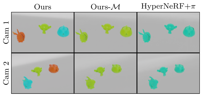
Figure 4: Novel view and novel attribute synthesis on synthetic data – We show examples of novel view and novel attribute synthesis on synthetic data. The scene is composed of three objects, where the color of each object is their attribute. Our method provides control over the color of each object independently, whereas both HyperNeRF+$\pi$ and Ours-$\mathcal{M}$ fail to deliver controllability and results in all three objects having the same attribute in the rendered scene.

Quantitative results on synthetic dataset

To complete the qualitative evaluation of our method, we provide results using synthetic dataset with available ground truth. We measure Peak Signal-to-Noise Ratio (PSNR), Multi-scale Structural Similarity (MS-SSIM) [44], and Learned Perceptual Image Patch Similarity (LPIPS) [50] and report them in Table 1. With only 5% of the annotations, our method provides the best novel-view and novel-attribute synthesis results, as reconfirmed by the qualitative examples in Figure 4. As shown, neither HyperNeRF+$\pi$ nor Ours-$\mathcal{M}$ is able to provide good results in this case, as without disentangled control of each attribute, the novel attribute and view settings of each test frame cannot be synthesized properly.

Interpolation task

To further verify that our rendering quality does not degrade with the introduction of controllability, we evaluate our method on a frame interpolation task without any attribute control. Unsurprisingly, as shown in Table 2, all methods that support dynamic scenes work similarly, including ours for interpolation. Note that for the interpolation task, we interpolate every other frame, in order to minimize the chance of attributes affecting the evaluation. Here, we are purely interested in the rendering quality from a novel view.

Method	PSNR $\uparrow$	MS-SSIM $\uparrow$	LPIPS $\downarrow$
NeRF	28.795	0.951	0.210
NeRF + Latent [30]	32.653	0.981	0.182
NeRFies [35]	32.274	0.981	0.180
HyperNeRF [36]	32.520	0.981	0.169
Ours-$\mathcal{M}$	32.061	0.979	0.167
Ours	32.342	0.981	0.168

Table 2: Quantitative results (interpolation) – We report results in terms of PSNR, MS-SSIM, and LPIPS for the interpolation task. These results are obtained for interpolated view synthesis only, not for novel attribute rendering. Our method provides similar performance in terms of rendering quality, but with controllability.

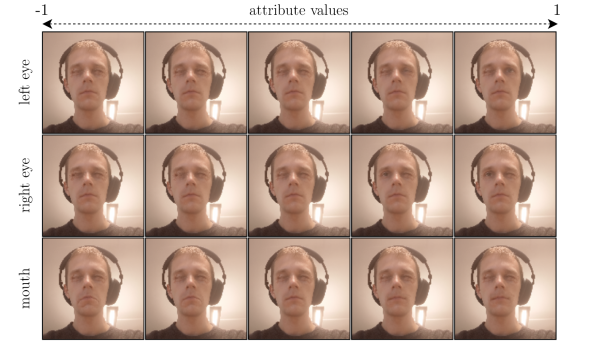
Figure 5: 2D image generation example – Our framework also generalizes to direct generation of 2D images. Here we show novel attribute synthesis for a webcam video of a person making expressions. Each individual part of the scene is correctly controlled according to the attribute values.

4.3 Direct 2D rendering

To verify how our approach generalizes beyond NeRF models and volume rendering, we apply our method to videos taken from a single view point, creating a 2D rendering task. We show in Figure 5 a proof-of-concept for employing our approach outside of NeRF applications to allow controllable neural generative models.

4.4 Ablation study

	Real (interpolation)			Synthetic (novel view & attr.)
Model	PSNR $\uparrow$	MS-SSIM $\uparrow$	LPIPS $\downarrow$	PSNR $\uparrow$	MS-SSIM $\uparrow$	LPIPS $\downarrow$
Base ($\mathcal{L}_{\text{recon}}$)	32.457	0.981	0.168	24.407	0.718	0.173
$+\mathcal{L}_{\text{enc}}$	32.478	0.982	0.167	27.018	0.871	0.164
$+\mathcal{L}_{\text{enc}}+\mathcal{L}_{\text{attr}}$	32.254	0.981	0.167	27.322	0.873	0.147
$+\mathcal{L}_{\text{enc}}+\mathcal{L}_{\text{attr}}+\mathcal{L}_{\text{mask}}$	32.342	0.981	0.168	32.394	0.972	0.139

Table 3: Effect of loss functions – We report the rendering quality of our method as we procedurally introduce the loss terms. For controlled rendering with novel views and attributes (synthetic data), each loss term adds to the rendering quality, with the $\mathcal{L}_{\text{mask}}$ being critical. For the novel view rendering on real data, addition of loss functions for controllability do not have a significant effect on the rendering quality—they do no harm.

Loss functions

In Table 3, we show how each loss term affects the network’s performance, contributing to performance improvements. When rendering novel views with novel attributes, the full formulation is a must, as without all loss terms the performance drops significantly—for example, results without $\mathcal{L}_{\text{mask}}$ is similar to Ours-$\mathcal{M}$ results in Table 1 and Figure 4. In the case of the interpolation task, the additional loss functions for controllability have no significant effect on the rendering quality. In other words, our controllability losses do not interfere with the rendering quality, other than imbuing the framework with controllability.

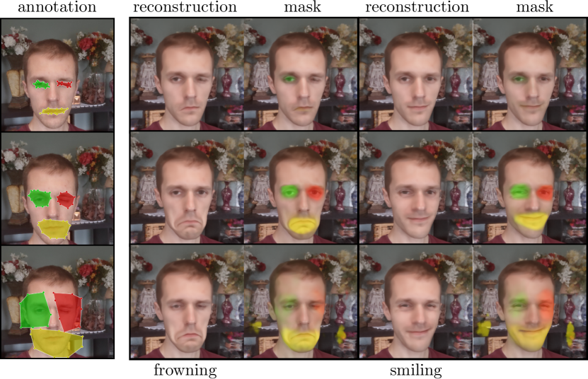
Figure 6: Effect of annotation quality – Our method is moderately robust to the quality of annotations. We visualize the results for two expressions: frowning and smiling, while keeping both eyes in a neutral position. Even with wildly varying annotations as shown, the reconstructions are reasonably controlled, with the exception of the top row, where we show a case where the annotations is too restrictive, resulting in the annotation being ignored for one eye. We show in bottom row also an interesting case, where the mask is large enough to start capturing the correlation among mouth expressions and the eye.

Quality of few shot supervision

We test how sensitive our method is against the quality of annotation supervision. In Figure 6 we demonstrate how each annotation leads to the final rendering quality. Our framework is robust to a moderate degree to the inaccuracies in the annotations. However, when they are too restrictive, the mask may collapse, as shown on the top row. Too large of a mask could also lead to moderate entanglement of attributes, as shown in the bottom row. Still, in all cases, our method provides a reasonable control over what is annotated.

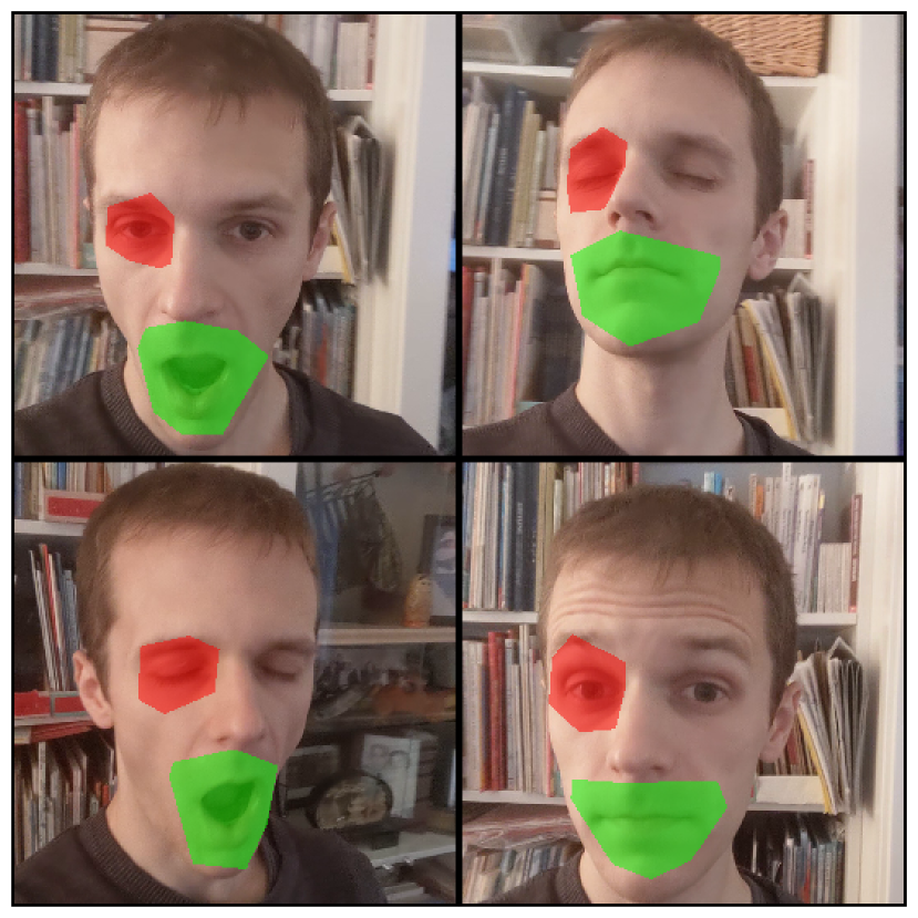
(a) annotated samples

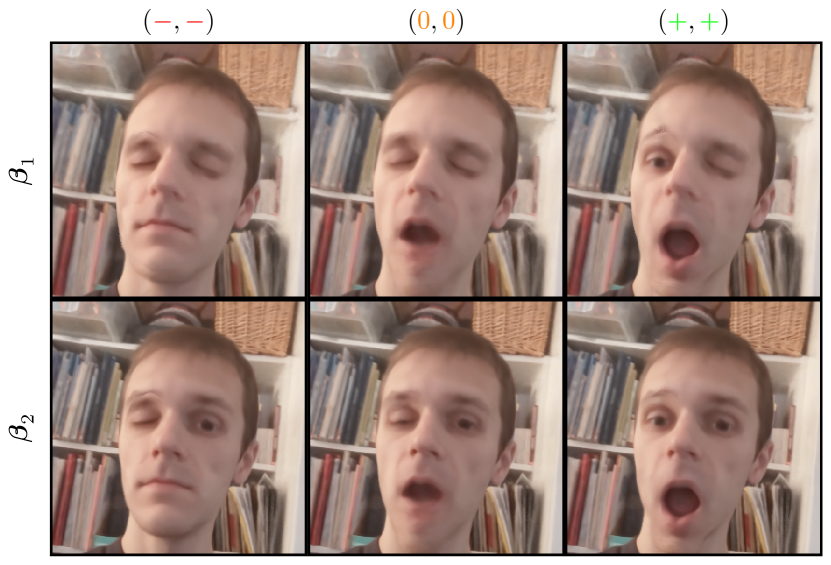
(b) renderings

Figure 7: Example with unannotated attributes – We show an example of how our method performs when a part of the image changes appearance, but is not annotated. With the annotations in (a), we synthesize the scene with novel view and attributes in (b), where the two rows are with different ${\boldsymbol{\beta}}$ configurations. We denote the attribute configuration on the top of each column in (b). As shown, the change that is not annotated is simply encoded in the per-image encoding ${\boldsymbol{\beta}}$.

Unannotated attributes

A natural question to ask is then what happens with the unannotated changes that may exist in the scene. In Figure 7 we show how the method performs when annotating only parts of the appearance change within the scene. The unannotated changes of the scene get encoded as ${\boldsymbol{\beta}}$, as in the case of HyperNeRF [36].

5 Conclusions

We have introduced CoNeRF, an intuitive controllable NeRF model that can be trained with few-shot annotations in the form of attribute masks. The core contribution of our method is that we represent attributes as localized masks, which are then treated as latent variables within the framework. To do so we regress the attribute and their corresponding masks with neural networks. This leads to a few-shot learning setup, where the network learns to regress provided annotations, and if they are not provided for a given image, proper attributes and masked are discovered throughout training automatically. We have shown that our method allows users to easily annotate what to control and how, within a single video simply by annotating a few frames, which then allows rendering of the scene from novel views and with novel attributes, at high quality.

Limitations

While our method delivers controllability to NeRF models, there is room for improvement. First, our disentanglement of attribute strictly relies on the locality assumption—if multiple attributes act on a single pixel, our method is likely to have entangled outcomes when rendering with different attributes. An interesting direction would therefore be to incorporate manifold disentanglement approaches [22, 51] to our method. Second, while very few, we still require sparse annotations. Unsupervised discovery of controllable attributes, for example as in [21], in a scene remains yet to be explored. Lastly, we resort to user intuition on which frames should be annotated—we heuristically choose frames with extreme attributes (e.g., mouth fully open). While this is a valid strategy, an interesting direction for future research would be to employ active learning techniques for this purpose [37, 6]

We further discuss potential societal impact of our work in the Supplementary Material.

6 Acknowledgements

We thank Thabo Beeler, JP Lewis, and Mark J. Matthews for their fruitful discussions, and Daniel Rebain for helping with processing the synthetic dataset. The work was partly supported by National Sciences and Engineering Research Council of Canada (NSERC), Compute Canada, and Microsoft Mixed Reality & AI Lab.

CoNeRF: Controllable Neural Radiance Fields
Supplementary Material

Appendix A Potential social impact

Our work is originally intended for creative and entertainment purposes, for example to allow users to easily edit their personal photos to have all the members of a group photo to have their eyes open. However, as with all work that enable editable models, our method has the potential to be misused for malicious purposes such as deep fakes. We strongly advise against such misuse. Recent work [5] has shown that it is possible to detect deep fakes, hinting that it should be possible to detect these deep learning-generated images. One of our future research direction is also along these lines, where we now aim to reliably detect images generated by our method.

Appendix B Architecture details

We present architecture of: canonicalizer ${\mathcal{K}}$ in Fig. 9, attribute map $\mathcal{A}$ in Fig. 10, hypermap $\mathcal{H}$ in Fig. 11, per-attribute hypermap in Fig. 12, mask prediction network in Fig. 13 and the rendering network in Fig. 14. Each network contains only fully connected layers. Hidden layers use ReLU activation function. Colors of figures correspond to colors of blocks in Fig. 1(b).

Appendix C Additional qualitative results

See attached video clip for more qualitative results.

Appendix D Failure Cases

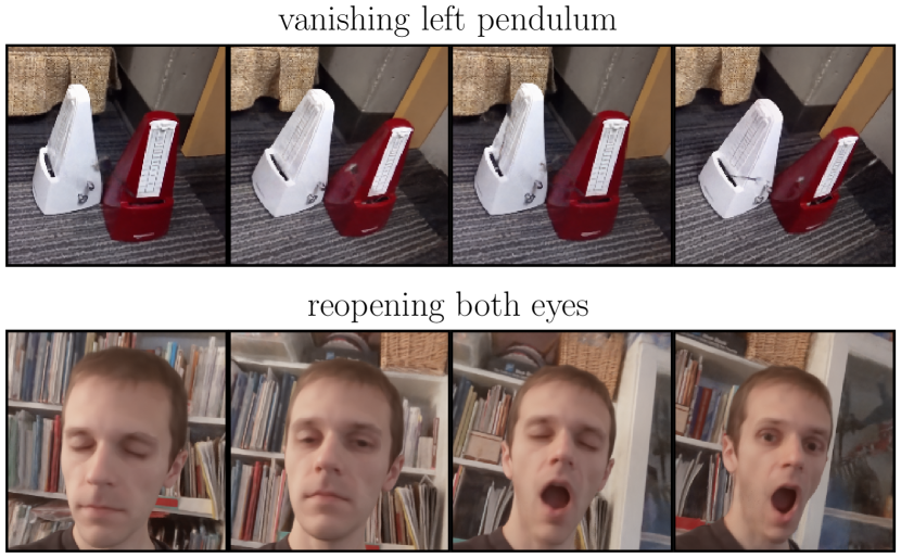
Figure 8: Failure cases – Our model may learn spurious interpolations for controlled elements that occupy little space in the image and with insufficient/careless annotations. For the metronome, due to the fast motion of the pendulum and its specularity, without careful annotation our method may simply learn its motion blur or sometimes even completely ignore the pendulum. In the face example, this may result in the eye blinking multiple times while interpolating between the attribute values of $-1$ and $1$. Both cases are preventable with more careful annotations and by annotating more frames.

We identify two modes of failure cases in our approach and present them in Fig. 8. In some cases with particular mask annotations, our model can struggle with controlling elements that occupy small space in the image. The problem is especially visible for controlling pendulum movement or opening and closing eyes. In the former, pendulum disappears and reappears in different places. In the latter, the control of eyes is periodic and there are two distant values in $[-1,1]$ that produce opening eyes. While with careful annotations we noticed that the problem is mostly preventable, this problem may occur in practice.

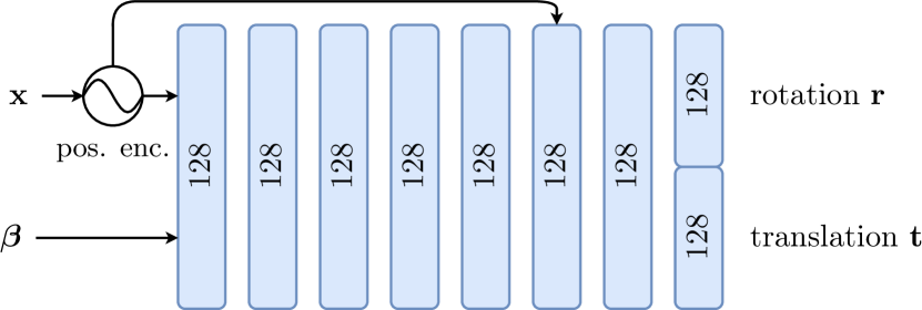
Figure 9: The canonicalization network takes positionally encoded raw coordinates ${\mathbf{x}}$ and learnable per-image latent code ${\boldsymbol{\beta}}$ and outputs rotation $\mathbf{r}$ expressed as a quaternion and translation $\mathbf{t}$. We rigidly transform each point ${\mathbf{x}}$ with an affine transform using both output. We use windowed positional encoding [35] for ${\mathbf{x}}$ with 8 components, linearly increasing contribution of components throughout 80k steps. We initialize the last layer to small values so the network can learn a base structure of the data.

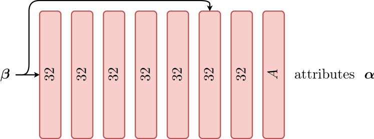
Figure 10: The attribute map $\mathcal{A}$ takes a per-image learnable latent code ${\boldsymbol{\beta}}$ and outputs $A$ attributes $\boldsymbol{\alpha}$.

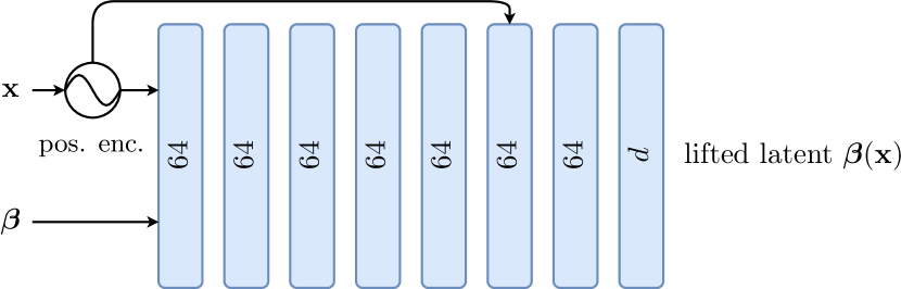
Figure 11: The network predicting lifted latent code ${\boldsymbol{\beta}}$, takes per-image ${\boldsymbol{\beta}}$ as an input, positionally encoded raw points ${\boldsymbol{\beta}}$ and outputs a lifted code of size $d$. We use only one sine component to encode ${\mathbf{x}}$.

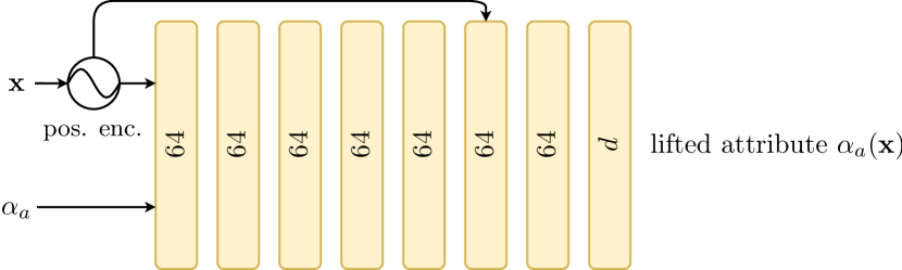
Figure 12: Per-attributes hypermaps take an attribute together with encoded ${\mathbf{x}}$ coordinates and output lifted $\alpha_{a}({\mathbf{x}})$ ambient code of size $d$. We encode ${\mathbf{x}}$ with only single component.

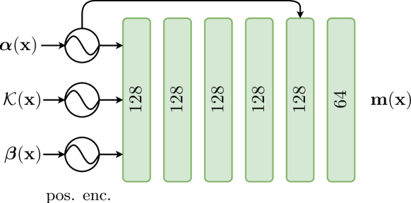
Figure 13: Masking network $\mathcal{M}$ take lifted attributes $\boldsymbol{\alpha}({\mathbf{x}})$, lifted latent code ${\boldsymbol{\beta}}({\mathbf{x}})$ and canonicalized points ${\mathcal{K}}({\mathbf{x}})$. We transform $\boldsymbol{\alpha}({\mathbf{x}})$ and ${\boldsymbol{\beta}}({\mathbf{x}})$ through a windowed positional encoding where we start at 1k-th step linearly increasing a single sine component for the next 10k steps. Points ${\mathcal{K}}({\mathbf{x}})$ are encoded with 8 components. The output is activated with a sigmoid function. We realize $\mathbf{m}_{0}({\mathbf{x}})$ as $\mathbf{m}({\mathbf{x}})_{0}=1-\sum_{a\in A}\mathbf{m}_{a}({\mathbf{x}})$, and clip the output to ensure the values range to be in $[0,1]$. Note that while the network shares similarities with the radiance field prediction part ${\mathcal{R}}$, it is not conditioned on view directions and appearance codes.

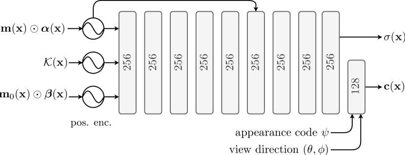
Figure 14: The radiance field prediction network predicts RGB colors $\mathbf{c}({\mathbf{x}})$ and density values $\sigma({\mathbf{x}})$ from canonicalized points. We encode points ${\mathbf{x}}$ with 8 sine components and linearly increase contribution of a single component in $\boldsymbol{\alpha}({\mathbf{x}})$ and ${\boldsymbol{\beta}}({\mathbf{x}})$ from 1k to 11k step. Per-point predicted predicted attributes $\boldsymbol{\alpha}({\mathbf{x}})$ and lifted latent code ${\boldsymbol{\beta}}({\mathbf{x}})$ are masked by a mask predicted from the masking network depicted in Fig. 13. The final linear layer takes additional per-image learnable appearance code $\psi$ to account for any visual variations that cannot be explained by the rest of the framework (e.g. changes in lighting). The code can discarded during evaluation. The same layer is additionally conditioned on the positionally encoded view directions. We activate the color output with a sigmoid function.

References

- [1] Bunny 3d model. https://graphics.stanford.edu/~mdfisher/Data/Meshes/bunny.obj. Accessed: 2021-11-16.
- [2] Suzanne 3d model. https://github.com/OpenGLInsights/OpenGLInsightsCode/blob/master/Chapter%2026%20Indexing%20Multiple%20Vertex%20Arrays/article/suzanne.obj. Accessed: 2021-11-16.
- [3] Teapot 3d model. https://graphics.stanford.edu/courses/cs148-10-summer/as3/code/as3/teapot.obj. Accessed: 2021-11-16.
- [4] Thiemo Alldieck, Hongyi Xu, and Cristian Sminchisescu. imGHUM: Implicit Generative Models of 3D Human Shape and Articulated Pose. In Conf. on Comput. Vis. Pattern Recognit., 2021.
- [5] Vishal Asnani, Xi Yin, Tal Hassner, and Xiaoming Liu. Reverse Engineering of Generative Models: Inferring Model Hyperparameters from Generated Images. ArXiv preprint, 2021.
- [6] Soufiane Belharbi, Ismail Ben Ayed, Luke McCaffrey, and Eric Granger. Deep Active Learning for Joint Classification & Segmentation with Weak Annotator. In IEEE Winter Conf. on Appl. of Comput. Vis., 2021.
- [7] Volker Blanz and Thomas Vetter. A Morphable Model for the Synthesis of 3D Faces. In Annual Conference on Computer Graphics and Interactive Techniques, 1999.
- [8] James Bradbury, Roy Frostig, Peter Hawkins, Matthew James Johnson, Chris Leary, Dougal Maclaurin, George Necula, Adam Paszke, Jake VanderPlas, Skye Wanderman-Milne, and Qiao Zhang. JAX: Composable Transformations of Python+NumPy Programs. http://github.com/google/jax, 2018.
- [9] Xi Chen, Yan Duan, Rein Houthooft, John Schulman, Ilya Sutskever, and Pieter Abbeel. InfoGAN: Interpretable Representation Learning by Information Maximizing Generative Adversarial Nets. In Adv. Neural Inf. Process. Syst., 2016.
- [10] Boyang Deng, John P Lewis, Timothy Jeruzalski, Gerard Pons-Moll, Geoffrey Hinton, Mohammad Norouzi, and Andrea Tagliasacchi. NASA: Neural Articulated Shape Approximation. In European Conf. on Comput. Vis., 2020.
- [11] Paul Ekman and Erika L Rosenberg. What the Face Reveals: Basic and Applied Studies of Spontaneous Expression Using the Facial Action Coding System (FACS). Oxford University Press, USA, 1997.
- [12] Guy Gafni, Justus Thies, Michael Zollhofer, and Matthias Nießner. Dynamic Neural Radiance Fields for Monocular 4D Facial Avatar Reconstruction. In Conf. on Comput. Vis. Pattern Recognit., 2021.
- [13] Klaus Greff, Andrea Tagliasacchi, Derek Liu, and Issam Laradji. Kubric. http://github.com/google-research/kubric, 2021.
- [14] Michelle Guo, Alireza Fathi, Jiajun Wu, and Thomas Funkhouser. Object-Centric Neural Scene Rendering. ArXiv preprint, 2020.
- [15] Tong He, Yuanlu Xu, Shunsuke Saito, Stefano Soatto, and Tony Tung. ARCH++: Animation-Ready Clothed Human Reconstruction Revisited. In Int. Conf. on Comput. Vis., 2021.
- [16] Irina Higgins, David Amos, David Pfau, Sebastien Racaniere, Loic Matthey, Danilo Rezende, and Alexander Lerchner. Towards a Definition of Disentangled Representations. ArXiv preprint, 2018.
- [17] Irina Higgins, Loic Matthey, Arka Pal, Christopher Burgess, Xavier Glorot, Matthew Botvinick, Shakir Mohamed, and Alexander Lerchner. beta-VAE: Learning Basic Visual Concepts with a Constrained Variational Framework. In Int. Conf. on Learn. Representations, 2017.
- [18] Wonbong Jang and Lourdes Agapito. CodeNeRF: Disentangled Neural Radiance Fields for Object Categories. In Int. Conf. on Comput. Vis., 2021.
- [19] James T Kajiya and Brian P Von Herzen. Ray Tracing Volume Densities. ACM SIGGRAPH Computer Graphics, 18(3):165–174, 1984.
- [20] Diederik P Kingma and Jimmy Ba. Adam: A Method for Stochastic Optimization. In Int. Conf. on Learn. Representations, 2014.
- [21] Tejas Kulkarni, Ankush Gupta, Catalin Ionescu, Sebastian Borgeaud, Malcolm Reynolds, Andrew Zisserman, and Volodymyr Mnih. Unsupervised Learning of Object Keypoints for Perception and Control. In Adv. Neural Inf. Process. Syst., 2019.
- [22] Stan Z Li, Zelin Zang, and Lirong Wu. Markov-Lipschitz Deep Learning. ArXiv preprint, 2020.
- [23] Tsung-Yi Lin, Priya Goyal, Ross Girshick, Kaiming He, and Piotr Dollár. Focal Loss for Dense Object Detection. In Int. Conf. on Comput. Vis., 2017.
- [24] Lingjie Liu, Marc Habermann, Viktor Rudnev, Kripasindhu Sarkar, Jiatao Gu, and Christian Theobalt. Neural Actor: Neural Free-view Synthesis of Human Actors with Pose Control. In ACM SIGGRAPH Asia, 2021.
- [25] Steven Liu, Xiuming Zhang, Zhoutong Zhang, Richard Zhang, Jun-Yan Zhu, and Bryan Russell. Editing Conditional Radiance Fields. ArXiv preprint, 2021.
- [26] Matthew Loper, Naureen Mahmood, Javier Romero, Gerard Pons-Moll, and Michael J. Black. SMPL: A Skinned Multi-Person Linear Model. ACM Trans. Graphics (Proc. SIGGRAPH Asia), 34(6):248:1–248:16, Oct. 2015.
- [27] Qianli Ma, Shunsuke Saito, Jinlong Yang, Siyu Tang, and Michael J Black. SCALE: Modeling Clothed Humans with a Surface Codec of Articulated Local Elements. In Conf. on Comput. Vis. Pattern Recognit., 2021.
- [28] Ricardo Martin-Brualla, Noha Radwan, Mehdi SM Sajjadi, Jonathan T Barron, Alexey Dosovitskiy, and Daniel Duckworth. NeRF in the Wild: Neural Radiance Fields for Unconstrained Photo Collections. In Conf. on Comput. Vis. Pattern Recognit., 2021.
- [29] Marko Mihajlovic, Yan Zhang, Michael J Black, and Siyu Tang. LEAP: Learning Articulated Occupancy of People. In Conf. on Comput. Vis. Pattern Recognit., 2021.
- [30] Ben Mildenhall, Pratul P Srinivasan, Matthew Tancik, Jonathan T Barron, Ravi Ramamoorthi, and Ren Ng. NeRF: Representing Scenes as Neural Radiance Fields for View Synthesis. In European Conf. on Comput. Vis., 2020.
- [31] Jiteng Mu, Weichao Qiu, Adam Kortylewski, Alan Yuille, Nuno Vasconcelos, and Xiaolong Wang. A-SDF: Learning Disentangled Signed Distance Functions for Articulated Shape Representation. In Int. Conf. on Comput. Vis., 2021.
- [32] Thomas Neumann, Kiran Varanasi, Stephan Wenger, Markus Wacker, Marcus Magnor, and Christian Theobalt. Sparse Localized Deformation Components. ACM Trans. on Graphics, 32(6):1–10, 2013.
- [33] Atsuhiro Noguchi, Xiao Sun, Stephen Lin, and Tatsuya Harada. Neural Articulated Radiance Field. In Int. Conf. on Comput. Vis., 2021.
- [34] Jeong Joon Park, Peter Florence, Julian Straub, Richard Newcombe, and Steven Lovegrove. DeepSDF: Learning Continuous Signed Distance Functions for Shape Representation. In Conf. on Comput. Vis. Pattern Recognit., 2019.
- [35] Keunhong Park, Utkarsh Sinha, Jonathan T Barron, Sofien Bouaziz, Dan B Goldman, Steven M Seitz, and Ricardo Martin-Brualla. Deformable Neural Radiance Fields. In Int. Conf. on Comput. Vis., 2021.
- [36] Keunhong Park, Utkarsh Sinha, Peter Hedman, Jonathan T Barron, Sofien Bouaziz, Dan B Goldman, Ricardo Martin-Brualla, and Steven M Seitz. HyperNeRF: A Higher-Dimensional Representation for Topologically Varying Neural Radiance Fields. ArXiv preprint, 2021.
- [37] Pengzhen Ren, Yun Xiao, Xiaojun Chang, Po-Yao Huang, Zhihui Li, Xiaojiang Chen, and Xin Wang. A Survey of Deep Active Learning. ACM Comput. Surveys, 2020.
- [38] Shunsuke Saito, Jinlong Yang, Qianli Ma, and Michael J Black. SCANimate: Weakly Supervised Learning of Skinned Clothed Avatar Networks. In Conf. on Comput. Vis. Pattern Recognit., 2021.
- [39] Katja Schwarz, Yiyi Liao, Michael Niemeyer, and Andreas Geiger. GRAF: Generative Radiance Fields for 3D-Aware Image Synthesis. In Adv. Neural Inf. Process. Syst., 2020.
- [40] Shih-Yang Su, Frank Yu, Michael Zollhöfer, and Helge Rhodin. A-NeRF: A-NeRF: Articulated Neural Radiance Fields for Learning Human Shape, Appearance, and Pose. In Adv. Neural Inf. Process. Syst., 2021.
- [41] Justus Thies, Michael Zollhofer, Marc Stamminger, Christian Theobalt, and Matthias Nießner. Face2Face: Real-time Face Capture and Reenactment of RGB Videos. In Conf. on Comput. Vis. Pattern Recognit., 2016.
- [42] Edgar Tretschk, Ayush Tewari, Vladislav Golyanik, Michael Zollhofer, Christoph Lassner, and Christian Theobalt. Non-Rigid Neural Radiance Fields: Reconstruction and Novel View Synthesis of a Dynamic Scene From Monocular Video. In Int. Conf. on Comput. Vis., 2021.
- [43] Alex Trevithick and Bo Yang. GRF: Learning a General Radiance Field for 3D Scene Representation and Rendering. In Int. Conf. on Comput. Vis., 2021.
- [44] Zhou Wang, Eero P Simoncelli, and Alan C Bovik. Multiscale Structural Similarity for Image Quality Assessment. In Asilomar Conference on Signals, Systems & Computers, 2003.
- [45] Chenglei Wu, Derek Bradley, Markus Gross, and Thabo Beeler. An Anatomically-Constrained Local Deformation Model for Monocular Face Capture. ACM Trans. on Graphics, 35(4):1–12, 2016.
- [46] Christopher Xie, Keunhong Park, Ricardo Martin-Brualla, and Matthew Brown. FiG-NeRF: Figure-Ground Neural Radiance Fields for 3D Object Category Modelling. In Int. Conf. on 3D Vis., 2021.
- [47] Bangbang Yang, Yinda Zhang, Yinghao Xu, Yijin Li, Han Zhou, Hujun Bao, Guofeng Zhang, and Zhaopeng Cui. Learning Object-Compositional Neural Radiance Field for Editable Scene Rendering. In Int. Conf. on Comput. Vis., 2021.
- [48] Hong-Xing Yu, Leonidas J Guibas, and Jiajun Wu. Unsupervised Discovery of Object Radiance Fields. ArXiv preprint, 2021.
- [49] Kai Zhang, Gernot Riegler, Noah Snavely, and Vladlen Koltun. NeRF++: Analyzing and Improving Neural Radiance Fields. ArXiv preprint, 2020.
- [50] Richard Zhang, Phillip Isola, Alexei A Efros, Eli Shechtman, and Oliver Wang. The Unreasonable Effectiveness of Deep Features as a Perceptual Metric. In Conf. on Comput. Vis. Pattern Recognit., 2018.
- [51] Sharon Zhang, Amit Moscovich, and Amit Singer. Product Manifold Learning. In Inter. Conf. on Artif. Intell. and Stat., 2021.
- [52] Xiuming Zhang, Pratul P Srinivasan, Boyang Deng, Paul Debevec, William T Freeman, and Jonathan T Barron. NeRFactor: Neural Factorization of Shape and Reflectance Under an Unknown Illumination. ArXiv preprint, 2021.
- [53] Zerong Zheng, Tao Yu, Yebin Liu, and Qionghai Dai. PaMIR: Parametric Model-Conditioned Implicit Representation for Image-based Human Reconstruction. IEEE Trans. on Pattern Anal. Mach. Intell., 2021.
- [54] Pierre Zins, Yuanlu Xu, Edmond Boyer, Stefanie Wuhrer, and Tony Tung. Data-Driven 3D Reconstruction of Dressed Humans From Sparse Views. In Int. Conf. on 3D Vis., 2021.